Assessment of an Implicit Discontinuous Galerkin Solver for Incompressible Flow Problems with Variable Density

Abstract

Multi-component flow problems are typical of many technological and engineering applications. In this work, we propose an implicit high-order discontinuous Galerkin discretization of the variable density incompressible (VDI) flow model for the simulation of multi-component problems. Indeed, the peculiarity of the VDI model is that the density is treated as an advected property, which can be used to possibly track multiple (more than two) components. The interface between fluids is described by a smooth, but sharp, variation in the density field, thus not requiring any geometrical reconstruction. Godunov numerical fluxes, density positivity, mass conservation, and Gibbs-type phenomena at material interfaces are challenges that are considered during the numerical approach development. To avoid Courant-related time step restrictions, high-order single-step multi-stage implicit schemes are applied for the temporal integration. Several test cases with known analytical solutions are used to assess the current approach in terms of space, time, and mass conservation accuracy. As a challenging application, the simulation of a 2D droplet impinging on a thin liquid film is performed and shows the capabilities of the proposed DG approach when dealing with high-density (water–air) multi-component problems.

1. Introduction

Multi-component flows are common in many industrial and technological processes. Extraction and transport of hydrocarbons, liquid jet machining, coating materials, fuel sprays, pollutants treatment, droplets dispersion, and porous media are just a few notable examples. Over the years, many numerical strategies have been developed to deal with such flow problems.

The first examples were given by the Lagrangian [1] and arbitrary Lagrangian–Eulerian methods [2]. The accuracies of these methods are very high but limited by the level of interface deformation, which may lead to severe mesh distortions. To reduce such distortions, front-tracking methods [3] were developed. They consider a fixed computational grid for the bulk flow and track the interface using Lagrangian tracers. Despite being less sensible to interface deformations, they become geometrically challenging as the deformation enlarges. To circumvent the aforementioned issues, other strategies, based on the Eulerian description of the flow field, were devised. In particular, the level-set method [4] and the volume of fluid method [5] are among the most successful ones. The former exploits the advection of a suitable function whose zero-level set denotes the interface. The latter tracks the free surface using a volume fraction variable and a geometrical reconstruction technique, e.g., the piecewise linear interface calculation [6].

All methods mentioned above treat the interface as a d-dimensional surface, with d being the problem dimension. A different interface-capturing approach is provided by diffuse interface methods [7,8,9,10], which allow the different fluid components to develop a thin mixing region, usually described as a smooth (but possibly sharp) variation of a field variable. Since no reconstruction or tracking of the interface is required, complex three-dimensional interface topologies with possible coalescence/break-up of droplets can easily be captured with no extra cost. In this context, the variable density incompressible (VDI) flow model [11] exhibits interesting features for the simulation of incompressible flow problems involving immiscible fluids of different densities. The interface between components is managed in a diffuse fashion as smooth variations of the density field. Due to the coexistence of the divergence constraint and the mass conservation, the density is treated as a purely advected property. Thus, it acts as a field variable, allowing it to distinguish different components of different densities.

As is the case for any diffuse interface method, the VDI flow model needs careful control of interface spreading to avoid meaningless descriptions of the flow problem under investigation. Numerical methods able to deliver high-order spatial accuracy are very attractive in this regard as they account for steep gradients of the field variable, thereby allowing to represent a sharp diffuse interface. Among the many high-order methods proposed in the literature, we focused on discontinuous Galerkin (DG) formulations, which are particularly well suited in the computational fluid dynamics context [12,13,14,15,16,17]. Indeed, they provide favorable dispersion and dissipation properties and the ability to achieve very high accuracy even on arbitrarily shaped polytopic mesh elements [18].

In this work, we investigated some numerical challenges involved in implicit high-order accurate DG discretizations of the VDI model introduced in [19] for the simulation of multi-component incompressible flow problems. This discretization follows the idea of coupling the artificial compressibility method to the VDI flow model [19,20,21,22,23,24] in order to introduce suitable Godunov fluxes at the inter-element boundaries. In particular, the formulation relies on the exact solution of local Riemann problems based on an artificial compressibility perturbation of the incompressible Navier–Stokes equations. Artificial compressibility is applied to recover a set of equations of the hyperbolic type and derive the exact Riemann problem solution by means of standard wave patterns [25]. We stress that the artificial compressibility acts only at the local Riemann problem level, while the set of governing equations still lacks the pressure time derivative. The coupling between pressure and velocity introduced by the Riemann solver allows for equal degree pressure-velocity formulations. Moreover, thanks to this coupling, the resulting space-discretized set of equations becomes a set of differential-algebraic equations (DAEs) of index 1, thus implicit high-order time integration schemes can be applied [26].

The assessment of the DG-VDI formulation conducted in this work focuses on the positivity of the discrete density field, the control of the Gibbs-type phenomena emerging from high-order representations of interfaces, and on the effectiveness of the time integration strategy.

Density positivity is crucial when dealing with multi-component flow problems featuring high-density ratios, e.g., water–air. The approach proposed in Section 3.3 consists of defining the density variable $\rho \in {\mathbb{R}}^{+}$ as the sole function of a discretized variable denoted as working density $\tilde{\rho }\in \mathbb{R}$ and enforcing density positivity by introducing a suitable variable transformation $\rho =f\left(\tilde{\rho }\right)$. Since the transformation introduces additional nonlinearities, accurate space and time integration strategies are required to guarantee mass conservation.

Gibbs-type phenomena emerge from high-order representations of sharp diffuse interfaces between components. Taking inspiration from shock-capturing techniques for compressible flows, we introduce an artificial mass diffusion source term within the set of equations which is activated by spurious oscillations, see Section 3.4. Despite being treated as a source term, this artificial diffusion is conservative since it leaves untouched the mean value of the conserved variable within each mesh element.

In Section 3.5, the set of DAEs is integrated in time with high-order single-step multi-stage ESDIRK schemes [27,28]. These nonlinear temporal schemes can be designed to have optimal stability properties, thus preventing Courant-related time step restrictions.

Section 4 presents the assessment in terms of space, time, and mass conservation accuracies of sets of governing equations on three test cases of known analytical solutions, and the simulation of the impingement of a 2D liquid (water) droplet on a thin film immersed in air. In Section 5, conclusions are given.

2. Variable Density Incompressible Flow Model

Let the computational domain $\Omega$ be a subset of the d-dimensional space; the model describing an incompressible flow of a Newtonian fluid with variable density is defined by augmenting the set of incompressible Navier–Stokes equations

$$\begin{array}{cc}\hfill {\displaystyle \frac{\partial u_j}{\partial x_j}}& =0,\hfill \\ \hfill \rho \frac{\mathrm{D}{u}_i}{\mathrm{D}t}& =-\frac{\partial p}{\partial x_i}+\frac{\partial {\tau }_{ij}}{\partial x_j}+\rho g_i,\hfill \end{array}$$

(1)

with the continuity equation

$$\frac{\partial \rho }{\partial t}+\frac{\partial }{\partial x_j}\left(\rho u_j\right)=0.$$

Suitable initial and boundary conditions must be introduced to complete the definition of the variable density incompressible flow problem. Above (and in what follows) equations are written in the Einstein notation and the spatial coordinates are described by means of a Cartesian reference frame. The ${\displaystyle \frac{\mathrm{D}(·)}{\mathrm{D}t}}$ is the material derivative.

Written in conservative form, the set of equations for the variable density incompressible (VDI) flow model reads

$$\begin{array}{cc}\hfill \frac{\partial u_j}{\partial x_j}& =0,\hfill \\ \hfill \frac{\partial }{\partial t}\left(\rho u_i\right)+\frac{\partial }{\partial x_j}\left(\rho u_i{u}_j\right)\hfill & \hfill =-\frac{\partial p}{\partial x_i}+\frac{\partial {\tau }_{ij}}{\partial x_j}+\rho g_i,\hfill \\ \hfill \frac{\partial \rho }{\partial t}+\frac{\partial }{\partial x_j}\left(\rho u_j\right)& =0,\hfill \end{array}$$

(2)

with $i,j=1,\cdots ,d$ and

$${\tau }_{ij}=2\mu \left[\frac{1}{2}\left(\frac{\partial u_i}{\partial x_j}+\frac{\partial u_j}{\partial x_i}\right)-\frac{1}{3}\frac{\partial u_k}{\partial x_k}{\delta }_{ij}\right].$$

The body acceleration is typically constant, e.g., gravitational acceleration, while the dynamic viscosity can be defined as a suitable function of the density $\mu =\mu \left(\rho \right)$.

The peculiar feature of the model in (2) lies in the simultaneous presence of the continuity equation and the divergence-free constraint, which leads to a null material derivative constraint for the density variable. In practice, the advected density variable can be employed as a phase variable. Accordingly, in the context of incompressible flow problems involving immiscible Newtonian fluids of different densities, e.g., water and air, the VDI flow model allows to discriminate different components simply by means of their different density values. Similarly, interfaces between components are identified in a diffuse fashion as smooth (and possibly sharp) variations of the density variable.

3. Numerical Framework

The model (2) can be written in compact form as

$$\mathit{D}\frac{\partial \mathit{q}}{\partial t}+\nabla ·{\mathit{F}}^c\left(\mathit{q}\right)+\nabla ·{\mathit{F}}^v(\mathit{q},\nabla \mathit{q})+\mathit{s}\left(\mathit{q}\right)=\mathbf{0},$$

where $\mathit{q}=\left\{p,\rho u_i,\rho \right\}\in {\mathbb{R}}^m$ is the vector of the $m=d+2$ conservative variables, ${\mathit{F}}^c,{\mathit{F}}^v\in {\mathbb{R}}^{m\times d}$ are the convective and viscous fluxes, $\mathit{s}\in {\mathbb{R}}^m$ is the source term, and $\mathit{D}=\mathit{I}-{\mathit{J}}^{11}\in {\mathbb{R}}^{m\times m}$ is the difference matrix between the identity matrix and a single-entry matrix, which takes into account the lack of pressure time derivative.

Alternative sets of variables, $\mathit{w}$, can be considered in place of the conservative one, $\mathit{q}$. Whenever this occurs, the following change of variable matrix has to be defined

$$\mathit{P}\left(\mathit{w}\right)={\displaystyle \frac{\partial \mathit{q}\left(\mathit{w}\right)}{\partial \mathit{w}}},$$

and the compact form of (2) becomes

$$\mathit{D}\mathit{P}\left(\mathit{w}\right)\frac{\partial \mathit{w}}{\partial t}+\nabla ·{\mathit{F}}^c\left(\mathit{w}\right)+\nabla ·{\mathit{F}}^v(\mathit{w},\nabla \mathit{w})+\mathit{s}\left(\mathit{w}\right)=\mathbf{0}.$$

(3)

Hereinafter, the generic set of variables $\mathit{w}$ is denoted as the set of working variables.

3.1. Discontinuous Galerkin Discretization

We are interested in the space discretization of the VDI flow model (3) using a high-order discontinuous Galerkin (DG) method. Let ${\mathcal{K}}_h=\left\{\mathrm{K}\right\}$ denote the collection of non-overlapping mesh elements K of the domain $\Omega \in {\mathbb{R}}^d$, such that

$${\overline{\Omega }}_h=\bigcup _{\mathrm{K}\in {\mathcal{K}}_h}\overline{\mathrm{K}}.$$

Let ${\mathcal{F}}_h=\left\{\mathrm{F}\right\}$ denote the set of faces of the computational mesh ${\Omega }_h$. ${\mathcal{F}}_h^b$ collects the faces at the boundary of ${\Omega }_h$ and ${\mathcal{F}}_h^i={\mathcal{F}}_h\backslash {\mathcal{F}}_h^b$ the internal faces, i.e., for any $\mathrm{F}\in {\mathcal{F}}_h^i$, there exist two elements ${\mathrm{K}}^{+},{\mathrm{K}}^{-}\in {\mathcal{K}}_h$, such that $\mathrm{F}\in \partial {\mathrm{K}}^{+}\cap \partial {\mathrm{K}}^{-}$.

Then, let us define the discrete polynomial space

$${\mathbb{P}}_d^k\left({\mathcal{K}}_h\right)=\left\{v_h\in L^2(\Omega )|v_h{}_{|\mathrm{K}}\in {\mathbb{P}}_d^k\left(\mathrm{K}\right),\forall \mathrm{K}\in {\mathcal{K}}_h\right\},$$

where $k\ge 0$ is an integer and ${\mathbb{P}}_d^k\left(\mathrm{K}\right)$ denotes the restriction to K of the polynomial functions of d variables and total degree $\le k$. For this polynomial space, a set of orthonormal and hierarchical basis functions is computed according to [29].

By multiplying Equation (3) by an arbitrary smooth test function $\mathit{v}=\left\{v_1,\cdots ,v_m\right\}$, and integrating by parts, we obtain the weak formulation

$$\begin{array}{l}{\int }_{\Omega }\mathit{v}·\left(\mathit{D}\mathit{P}\left(\mathit{w}\right)\frac{\partial \mathit{w}}{\partial t}\right)\mathrm{d}\mathit{x}-{\int }_{\Omega }\nabla \mathit{v}:\left[{\mathit{F}}^c\left(\mathit{w}\right)+{\mathit{F}}^v\left(\mathit{w},\nabla \mathit{w}\right)\right]\mathrm{d}\mathit{x}\\ \hspace{1em}\hspace{1em}\hspace{1em}\hspace{1em}\hspace{1em}\hspace{1em}\hspace{1em}\hspace{1em}+{\oint }_{\partial \Omega }\mathit{v}\otimes \mathit{n}:\left[{\mathit{F}}^c\left(\mathit{w}\right)+{\mathit{F}}^v\left(\mathit{w},\nabla \mathit{w}\right)\right]\mathrm{d}\mathit{x}+{\int }_{\Omega }\mathit{v}·\mathit{s}\left(\mathit{w}\right)\mathrm{d}\mathit{x}=0,\end{array}$$

(4)

where $\mathit{n}$ is the unit vector normal to the boundary.

In order to discretize Equation (4) by means of discontinuous Galerkin methods, the solution $\mathit{w}$ and the test function $\mathit{v}$ are replaced with a finite element approximation ${\mathit{w}}_h$ and a discrete test function ${\mathit{v}}_h$, respectively, both of which belong to ${\left[{\mathbb{P}}_d^k\left({\mathcal{K}}_h\right)\right]}^m$. Accordingly, within each mesh element $\mathrm{K}\in {\mathcal{K}}_h$ each component ${w_h}_j$, $j=1,\cdots ,m$, of ${\mathit{w}}_h$ can be expressed as

$${w_h}_j={\varphi }_l{W}_{jl},$$

where ${\varphi }_l$ are the orthonormal and hierarchical basis functions and $W_{jl}$ are the components of the global vector $\mathbf{W}$ of the unknown degrees of freedom (dof), being $l=1,\cdots ,N_{dof}^k$. As a generic function, ${\phi }_h\in {\mathbb{P}}_d^k\left({\mathcal{K}}_h\right)$ is double-valued over an internal mesh face and the jump trace operator $\left[\left[{\phi }_h\right]\right]={\phi }_h{{|}_{{\mathrm{K}}^{+}}-{\phi }_h|}_{{\mathrm{K}}^{-}}$ is introduced. Whenever applied to a vector, this operator acts component-wise.

The DG discretization of the governing equations consists in seeking, for $i=1,\cdots ,N_{dof}^k$ and $j=1,\cdots ,m$, the components of $\mathbf{W}$ such that

$$\begin{array}{c}\hspace{1em} \hspace{1em} \sum _{\mathrm{K}}{\int }_{\mathrm{K}}{\varphi }_i{D}_{ja}{P}_{ak}\left({\mathit{w}}_h\right){\varphi }_l\frac{\mathrm{d}{W}_{kl}}{\mathrm{d}t}\mathrm{d}\mathit{x}\hfill \\ \hspace{1em} \hspace{1em}-\sum _{\mathrm{K}}{\int }_{\mathrm{K}}\frac{\partial {\varphi }_i}{\partial x_b}\left[F_{jb}^c\left({\mathit{w}}_h\right)+F_{jb}^v\left({\mathit{w}}_h,{\nabla }_h{\mathit{w}}_h+\mathit{r}\left(\left[\left[{\mathit{w}}_h\right]\right]\right)\right)\right]\mathrm{d}\mathit{x}\\ \hspace{1em}\hspace{1em}\hspace{1em}\hspace{1em}+\sum _{\mathrm{F}}{\int }_{\mathrm{F}}\left[\left[{\varphi }_i\right]\right]n_b\left[{{\widehat{F}}^c}_{jb}\left({\mathit{w}}_h^{\pm }\right)+{{\widehat{F}}^v}_{jb}\left({\mathit{w}}_h^{\pm },{\left({\nabla }_h{\mathit{w}}_h+{\eta }_{\mathrm{F}}{\mathit{r}}_{\mathrm{F}}\left(\left[\left[{\mathit{w}}_h\right]\right]\right)\right)}^{\pm }\right)\right]\mathrm{d}\mathit{x}\\ \hspace{1em}\hspace{1em}\hspace{1em}\hspace{1em}\hspace{1em}\hspace{1em}\hspace{1em}\hspace{1em}\hspace{1em}\hspace{1em}\hspace{1em}\hspace{1em}\hspace{1em}\hspace{1em}\hspace{1em}\hspace{1em}\hspace{1em}\hspace{1em}\hspace{1em}\hspace{1em}\hspace{1em}\hspace{1em}\hspace{1em}\hspace{1em}\hspace{1em}\hspace{1em} +\sum _{\mathrm{K}}{\int }_{\mathrm{K}}{\varphi }_i{s}_j\left({\mathit{w}}_h\right)\mathrm{d}\mathit{x}=0_{ij}.\hfill \end{array}$$

(5)

Repeated indices imply summation over ranges $a,k=1,\cdots ,m$, $l=1,\cdots ,N_{dof}^k$, $b=1,\cdots ,d$. The residual of the DG discretization in (5) is a vector, in particular for each $j=1,\cdots ,m$ and all $i=1,\cdots ,N_{dof}^k$ we obtain the residual entries associated with the j-th equation of the VDI model in (3).

For the space discretization of the second-order terms, we rely on the second scheme of Bassi and Rebay (BR2) [30,31], where the viscous numerical flux is given by

$${\widehat{\mathit{F}}}^v\left({\mathit{w}}_h^{\pm },{\left({\nabla }_h{\mathit{w}}_h+{\eta }_{\mathrm{F}}{\mathbf{r}}_{\mathrm{F}}\left(\left[\left[{\mathit{w}}_h\right]\right]\right)\right)}^{\pm }\right)=\left\{{\mathit{F}}^v\left({\mathit{w}}_h,{\nabla }_h{\mathit{w}}_h+{\eta }_{\mathrm{F}}{\mathbf{r}}_{\mathrm{F}}\left(\left[\left[{\mathit{w}}_h\right]\right]\right)\right)\right\},$$

where $\left\{\phi \right\}=0.5\left({\phi }_h{{|}_{{\mathrm{K}}^{+}}+{\phi }_h|}_{{\mathrm{K}}^{-}}\right)$ is the average operator. $\mathbf{r}$ and ${\mathbf{r}}_{\mathrm{F}}$ are global and local lifting operators, respectively, and ${\eta }_{\mathrm{F}}$ is the stability parameter defined according to [31]. The convective numerical flux ${\widehat{F}}^c$ is computed as a Godunov flux using the exact Riemann solvers for VDI flows proposed by Bassi et al. [22].

A further integration by parts of the equation (5) leads to the so-called strong formulation [32]. In the current work, the strong formulation is adopted for the convective flux contribution while the weak formulation is considered for the viscous flux treatment.

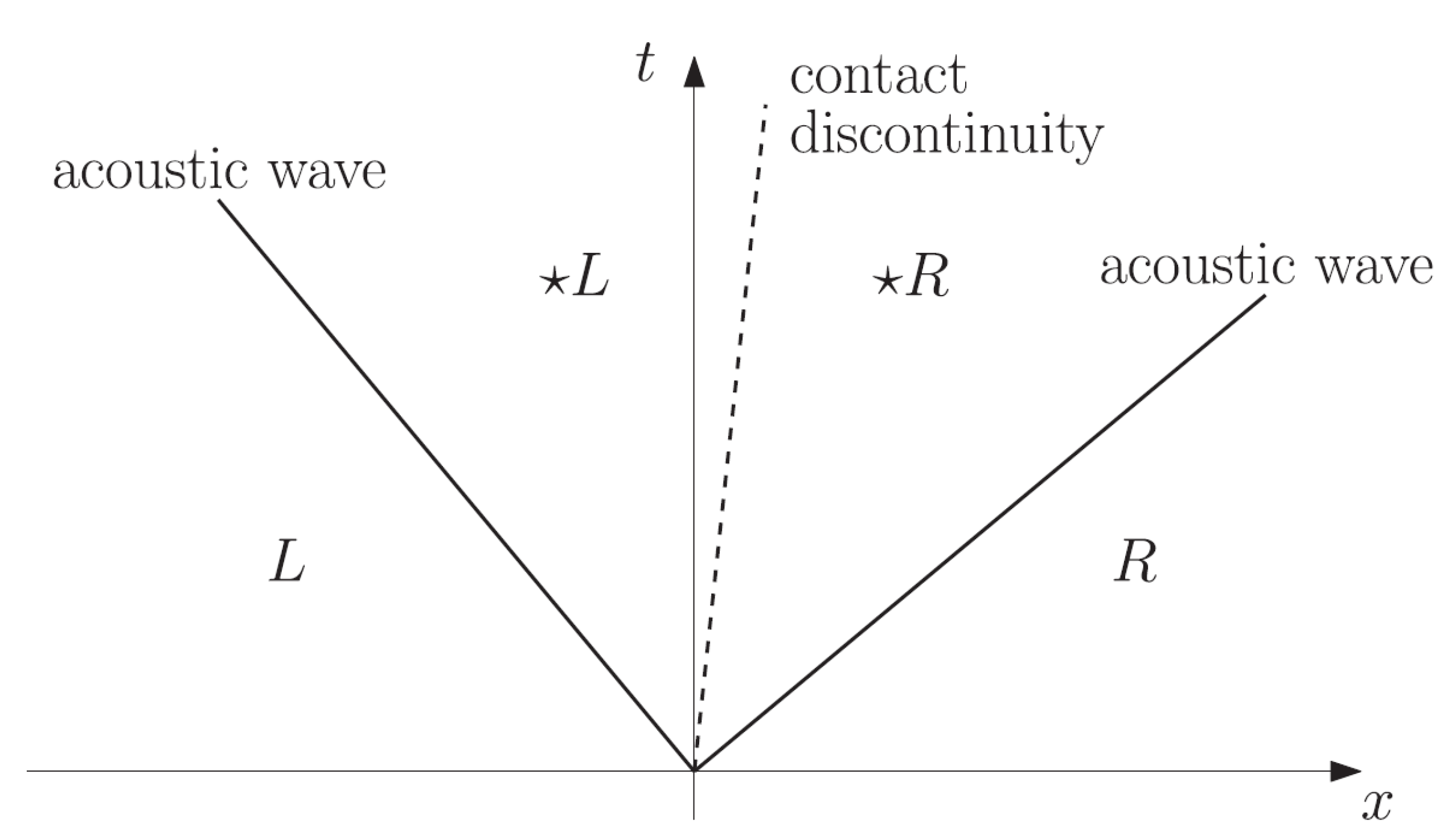
3.2. Riemann Solvers

The DG discretization of (3) requires the definition of suitable convective numerical fluxes ${\widehat{F}}^c$. To this end, in this work, we rely on Godunov fluxes based on the exact solution of Riemann solvers specifically conceived for VDI flows: we consider in particular the switched density Riemann solver (SDRS) and the exact Riemann solver (ERS) proposed in [22]. Both solvers aim to find a solution to the d-dimensional VDI inviscid equations split in the $\mathit{n}$-direction, where $\mathit{n}=\left\{n_1,\cdots ,n_d\right\}$ is the unit normal at point ${\mathit{x}}_0$ located on the mesh skeleton, i.e., ${\mathit{x}}_0\in {\bigcup }_{\mathrm{F}\in {\mathcal{F}}_h}\mathrm{F}$.

Let $x_n=x_i{n}_i$ and $u_n=u_i{n}_i$, be the normal components of the position and velocity vector, respectively, and let ${\mathit{u}}_{\theta }=\mathit{u}-u_n\mathit{n}$ be the tangential velocity vector. The set of $\mathit{n}$-split VDI equations

$$\begin{array}{cc}\hfill {\displaystyle \frac{\partial u_n}{\partial x_n}}& \hfill =0,\hfill \\ \hfill {\displaystyle \frac{\partial }{\partial t}}\left(\rho u_n\right)+{\displaystyle \frac{\partial }{\partial x_n}}\left(\rho u_n^2+p\right)& \hfill =0,\hfill \\ \hfill {\displaystyle \frac{\partial }{\partial t}}\left(\rho {\mathit{u}}_{\theta }\right)+{\displaystyle \frac{\partial }{\partial x_n}}\left(\rho {\mathit{u}}_{\theta }{u}_n\right)& \hfill =0,\hfill \\ \hfill {\displaystyle \frac{\partial \rho }{\partial t}}+{\displaystyle \frac{\partial }{\partial x_n}}\left(\rho u_n\right)& \hfill =0,\hfill \end{array}$$

(6)

coupled with initial piece-wise constant data

$$\left[p,u_n,{\mathit{u}}_{\theta },\rho \right]\left(x_n,t_0\right)=\left\{\begin{array}{cc}\hfill \left[p_L,{u_n}_L,{{\mathit{u}}_{\theta }}_L,{\rho }_L\right]\hfill & \hfill x_n<{x_n}_0,\hfill \\ \hfill \left[p_R,{u_n}_R,{{\mathit{u}}_{\theta }}_R,{\rho }_R\right]\hfill & \hfill x_n>{x_n}_0,\hfill \end{array}\right.$$

(7)

is the Riemann problem we ought to find a solution to. In (7), ${x_n}_0\in \mathrm{F}$ denotes the position of the discontinuity at initial time $t_0$, and the subscripts L (left) and R (right) denote the states of the two mesh elements ${\mathrm{K}}^{+}$ and ${\mathrm{K}}^{-}$ sharing F. According to the Godunov scheme approach, the solution at the locus $\mathcal{S}=(x_n-{x_n}_0)/t=0$ (vertical axis of Figure 1) is directly employed to evaluate the convective numerical fluxes.

Figure 1. Structure of the Riemann problem solution.

Since the system (6) does not fit into the framework of first-order hyperbolic conservation laws, the hyperbolic wave pattern solving the Riemann problem cannot be found. In order to overcome the issue, both SDRS and ERS rely on an artificial compressibility perturbation of (6), which, taking inspiration from the artificial compressibility model by Chorin [33], consists of adding a pressure time derivative to the first equation. The set of $\mathit{n}$-split equations for the SDRS reads

$$\begin{array}{cc}\hfill {\displaystyle \frac{1}{{\rho }_0{a}_0^2}}{\displaystyle \frac{\partial p}{\partial t}}+{\displaystyle \frac{\partial u_n}{\partial x_n}}& \hfill =0,\hfill \\ \hfill {\displaystyle \frac{\partial }{\partial t}}\left(\rho u_n\right)+{\displaystyle \frac{\partial }{\partial x_n}}\left(\rho u_n^2+p\right)& \hfill =0,\hfill \\ \hfill {\displaystyle \frac{\partial {\mathit{u}}_{\theta }}{\partial t}}+u_n{\displaystyle \frac{\partial {\mathit{u}}_{\theta }}{\partial x_n}}& \hfill =0,\hfill \\ \hfill {\displaystyle \frac{\partial \rho }{\partial t}}+u_n{\displaystyle \frac{\partial \rho }{\partial x_n}}& \hfill =0,\hfill \end{array}$$

(8)

while the set of $\mathit{n}$-split equations for the ERS reads

$$\begin{array}{cc}\hfill {\displaystyle \frac{1}{{\rho }_0{a}_0^2}}{\displaystyle \frac{\partial p}{\partial t}}+{\displaystyle \frac{\partial u_n}{\partial x_n}}& \hfill =0,\hfill \\ \hfill {\displaystyle \frac{\partial }{\partial t}}\left(\rho u_n\right)+{\displaystyle \frac{\partial }{\partial x_n}}\left(\rho u_n^2+p\right)& \hfill =0,\hfill \\ \hfill {\displaystyle \frac{\partial {\mathit{u}}_{\theta }}{\partial t}}+u_n{\displaystyle \frac{\partial {\mathit{u}}_{\theta }}{\partial x_n}}& \hfill =0,\hfill \\ \hfill {\displaystyle \frac{\partial \rho }{\partial t}}+{\displaystyle \frac{\partial }{\partial x_n}}\left(\rho u_n\right)& \hfill =0,\hfill \end{array}$$

(9)

where ${\rho }_0$ is the reference density and $a_0$ is the artificial compressibility parameter. Following [22], we set $a_0$ equal to the reference velocity employed in the definition of the non-dimensional groups, i.e., a unitary value of the dimensionless $a_0$. According to the third equation in (8) and (9), the tangential component of the velocity ${\mathit{u}}_{\theta }$ is purely advected along the normal direction. Since this equation is just the combination of the third and fourth equations of system (6), it does not represent a modification of the original set of $\mathit{n}$-split equations. Moreover, we underline that SDRS enforces the divergence constraint within the continuity equation, thus treating the density as an advected property along the normal direction.

The solution of the two Riemann problems (8), (7) and (9), (7), obtained by coupling the artificial compressibility perturbations of (8) with discontinuous initial data, consists of four constant states separated by two external acoustic waves and a central contact discontinuity, see Figure 1.

Depending on the external states (7), the acoustic waves can be either rarefactions or shocks, thus entailing a change of all flow properties that are not purely advected.The intermediate region embraced by the acoustic waves, denoted as the star region [25], is split into a left ($\star L$) and a right ($\star R$) portion by the contact discontinuity, across which pressure and normal velocity $u_n$ are constant.

We refer to Appendixes A and B of [22] for a complete derivation of the solution for the SDRS and the ERS. Interestingly, while the former requires solving a nonlinear equation system, the latter admits an explicit solution, resulting in better computational efficiency. As a peculiar feature of SDRS we mention that, since the density is purely advected, the density solution at $\mathcal{S}=0$ is equal either to the left or the right initial values. Accordingly, the density solution is guaranteed to never exceed the density values of the external states (7). As will be pointed out in Section 3.3, this latter feature is of crucial importance when using the Riemann solvers in combination with specific working variables $\mathit{w}$ choices.

3.3. Set of Working Variables

We consider the following set of working variables

$$\mathit{w}=\left\{p,u_i,\tilde{\rho }\right\},$$

(10)

which comprises the pressure p, the velocity components $u_{i=1,\cdots ,d}$ and the working density$\tilde{\rho }$, such that $\rho =f\left(\tilde{\rho }\right)$. Hence, in two space dimensions ($d=2$) the change of the variable matrix reads

$$\mathit{P}\left(\mathit{w}\right)=\frac{\partial \mathit{q}}{\partial \mathit{w}}=\left[\begin{array}{cccc}1& 0& 0& 0\\ 0& \rho & 0& {\rho }_{\tilde{\rho }}{u}_1\\ 0& 0& \rho & {\rho }_{\tilde{\rho }}{u}_2\\ 0& 0& 0& {\rho }_{\tilde{\rho }}\end{array}\right],$$

where ${\rho }_{\tilde{\rho }}=\mathrm{d}\rho /\mathrm{d}\tilde{\rho }$.

In this work, we consider three alternatives for the definition of $\tilde{\rho }$, exploiting the change of variable to enforce particular properties of the density field at the discrete level:

• linear

  $$\rho =f_1\left(\tilde{\rho }\right)=\tilde{\rho };$$

  (11)
• exponential

  $$\rho =f_2\left(\tilde{\rho }\right)={\mathrm{e}}^{{\sigma }_s\tilde{\rho }};$$

  (12)
• hyperbolic tangent-based

  $$\rho =f_3\left(\tilde{\rho }\right)={\displaystyle \frac{r_{\rho }+1+\left(r_{\rho }+1\right)tanh\left({\sigma }_s\tilde{\rho }\right)}{2r_{\rho }}}.$$

  (13)

In Equation (13), $r_{\rho }={\rho }_{+}/{\rho }_{-}$ is the maximum density ratio occurring in the density field, with ${\rho }_{+}$ and ${\rho }_{-}$ the maximum and minimum density values for the flow problem at hand, respectively. In Equations (12) and (13), ${\sigma }_s\in \mathbb{R}\backslash \left\{0\right\}$ is a scaling factor defined as follows

$${\sigma }_s=max\left[{\displaystyle \frac{1}{{\Delta }_{\tilde{\rho }}}}ln\left(r_{\rho }\right),1\right],$$

where ${\Delta }_{\tilde{\rho }}=\tilde{\rho }\left({\rho }_{+}\right)-\tilde{\rho }\left({\rho }_{-}\right)$ is a user-defined range. In this work, we consider ${\Delta }_{\tilde{\rho }}=1$. The max function is introduced to gracefully deal with unit density ratios. Notice that in (11)–(13) the density has to be indented dimensionless with respect to the reference density ${\rho }_0={\rho }_{+}$.

According to the linear transformation (11) the set of working variables falls back to the set of primitive variables, hence no particular properties are enforced at the discrete level. Instead, the exponential (12) and the hyperbolic tangent (13) based transformations restrict the range of admissible density values as follows

$$f_2\left(\tilde{\rho }\right):\mathbb{R}\to \left(0,+\infty \right)\mathrm{and}{f}_3\left(\tilde{\rho }\right):\mathbb{R}\to \left(0,1+{\displaystyle \frac{1}{r_{\rho }}}\right).$$

thereby ensuring density positivity at the discrete level. Interestingly, by controlling the maximum density value, the hyperbolic tangent transformation in (13) also provides the ability to limit density over/under-shoots associated with high-order approximations of steep density gradients in multi-component flow problems. Nevertheless, it must be clear that Gibbs-type phenomena promoting such over/under-shoots are not eliminated. As detailed in Section 3.4, proper treatment is required to avoid simulation blow up. Moreover, when employing the hyperbolic tangent transformation, in order to avoid failure of the inverse transformation $\tilde{\rho }=f_3^{-1}\left(\rho \right)$, it must be ensured that $\rho \in \left(0,1+1/r_{\rho }\right)$. Since the inverse transformation is applied to the density obtained from the Riemann solver in order to retrieve the working density to be plugged into the convective numerical flux, it is mandatory to rely on the SDRS. Indeed, as detailed in Section 3.2, only SDRS ensures that the star region density falls within the external states limits. Note that external density values computed from $\tilde{\rho }$ are within the limits by construction. Note that ERS is well suited to be used in combination with $f_1\left(\tilde{\rho }\right)$ and $f_2\left(\tilde{\rho }\right)$ transformations.

Despite its appealing features, it is important to point out that the change of density variable introduces strong nonlinearities within the system (3) and, hand-in-hand, in the DG discretized problem (5). Accordingly, the conservation of relevant physical quantities is subdued to the ability to accurately integrate the nonlinearities, in both space and time.

3.4. Shock Capturing for Material Interfaces

The VDI flow model allows dealing with incompressible flow problems involving immiscible fluids of different densities, e.g., water and air. Different fluid components are discriminated through the density, which acts as a phase variable, and the interface between components is represented as a sharp variation of the density field. It is well known that high-order discretizations are affected by Gibbs-type phenomena in the presence of excessively sharp gradients. This might endow a lack of monotonicity at interfaces, which must be properly controlled to avoid stability issues. In this work, we implemented a strategy based on the introduction of artificial viscosity inspired by the approach proposed by Persson and Peraire [34] in the context of compressible flows featuring shocks.

In the context of the VDI flow model, spurious density oscillations might occur at contact discontinuities. Accordingly, the artificial diffusive term is introduced solely within the continuity equation

$$\frac{\partial \rho }{\partial t}+\frac{\partial }{\partial x_j}\left(\rho u_j\right)=\frac{\partial }{\partial x_j}\left({\nu }_{ϵ}\frac{\partial \rho }{\partial x_j}\right).$$

Nevertheless, in order to ensure that the momentum equation of (1) is actually solved, we propose the following conservative form of the VDI flow model with artificial viscosity:

$$\begin{array}{cc}\hfill \frac{\partial u_j}{\partial x_j}& =0,\hfill \\ \hfill \frac{\partial }{\partial t}\left(\rho u_i\right)+\frac{\partial }{\partial x_j}\left(\rho u_i{u}_j\right)& \hfill =-\frac{\partial p}{\partial x_i}+\frac{\partial {\tau }_{ij}}{\partial x_j}+\rho g_i+u_i\frac{\partial }{\partial x_j}\left({\nu }_{ϵ}\frac{\partial \rho }{\partial x_j}\right),\hfill \\ \hfill \frac{\partial \rho }{\partial t}+\frac{\partial }{\partial x_j}\left(\rho u_j\right)& =\frac{\partial }{\partial x_j}\left({\nu }_{ϵ}\frac{\partial \rho }{\partial x_j}\right),\hfill \end{array}$$

(14)

with $i,j=1,\cdots ,d$ and ${\nu }_{ϵ}$ is the artificial mass diffusion parameter.

In order to ensure that artificial mass diffusion is introduced only at interfaces, we rely on a smoothness sensor based on the modal decay of the working density $\tilde{\rho }$ expansion. The artificial diffusion ${\nu }_{ϵ}$ is, thus, defined according to [34] as

$${\nu }_{ϵ}=\left\{\begin{array}{cc}{\nu }_{ϵ0}\hfill & \mathrm{if}s<s_0-\Delta s\hfill \\ {\displaystyle \frac{{\nu }_{ϵ0}}{2}}\left[1+sin\left({\displaystyle \frac{\pi }{2}}{\displaystyle \frac{s_0-s}{\Delta s}}\right)\right]\hfill & \mathrm{if}{s}_0-\Delta s\le s\le s_0+\Delta s\hfill \\ 0\hfill & \mathrm{otherwise}.\hfill \end{array}\right.$$

where the smoothness sensor s is defined according to the skyline pessimization procedure proposed by Klöckner et al. [35]. According to [35], $s\gg 1$ when the field is smooth and $s\approx 1$ when the density field exhibits abrupt variations. The user-defined parameters $s_0$ and $\Delta s$ define the threshold triggering the introduction of artificial viscosity as well as the actual amount of artificial viscosity introduced, which varies from 0 to ${\nu }_{ϵ}$. In this work, we set $s_0=1$, $\Delta s=0.75$ and ${\nu }_{ϵ0}=h/k$, with h the mesh element size and k the DG polynomial degree. This choice aims to introduce artificial diffusion that decreases with higher polynomial degrees and smaller elements, allowing to possibly capture discontinuities as thin layers within a single mesh element. A sufficiently high polynomial degree, namely $k\ge 4$, is required to ensure that the modal decay provides a reliable smoothness sensor.

The two additional terms related to artificial diffusion appearing in (14), one within the continuity equation and one within the momentum equation, are discretized in space following the idea proposed by Jaffre et al. [36]. In particular, the additional term within the continuity equation is discretized by multiplying by an arbitrary test function, integrating by parts and neglecting the numerical flux contributions on the inter-element boundaries. Accordingly, the following term has to be included in (5) for the DoFs ($i=1,\cdots ,N_{dof}^k$) related to the continuity equation ($j=d+2$)

$$\sum _{\mathrm{K}}{\int }_{\mathrm{K}}\frac{\partial {\varphi }_i}{\partial x_b}{\nu }_{ϵ}\frac{\partial \rho }{\partial x_b}\mathrm{d}\mathit{x}.$$

(15)

The additional term within the momentum equation is discretized in a consistent way with respect to (15). Thus, for $i=1,\cdots ,N_{dof}^k$ and $j=2,\cdots ,d+1$, the following contribution is included in (5)

$$\sum _{\mathrm{K}}{\int }_{\mathrm{K}}\frac{\partial {\varphi }_i}{\partial x_b}{u}_{j-1}{\nu }_{ϵ}\frac{\partial \rho }{\partial x_b}\mathrm{d}\mathit{x}.$$

(16)

It is interesting to note that, despite the introduction of (15) and (16), the resulting DG formulation is conservative. Indeed, keeping in mind that we rely on a set of hierarchical modal basis functions, for the first degree of freedom ($i=1$), it holds

$${\displaystyle \frac{\partial {\varphi }_1}{\partial x_b}}=0.$$

with $b=1,\cdots ,d$. Since the first degree of freedom defines the average value of the conservative variable in each mesh element, it is clear that the proposed DG discretization of the artificial diffusion terms leads to a conservative formulation.

3.5. Implicit Time Integration

The numerical integration of Equation (5) by means of suitable Gaussian quadrature rules leads to a semi-discrete system of nonlinear differential-algebraic equations that can be compactly rewritten as follows

$${\mathbf{M}}_{\mathit{P}}\left(\mathbf{W}\right){\displaystyle \frac{\mathrm{d}\mathbf{W}}{\mathrm{d}t}}+\mathbf{R}\left(\mathbf{W}\right)=\mathbf{0},$$

(17)

where ${\mathbf{M}}_{\mathit{P}}\left(\mathbf{W}\right)$ is the global block diagonal mass matrix derived from the discretization of the first integral in Equation (5) and $\mathbf{R}\left(\mathbf{W}\right)$ is the global residual vector pertaining to all of the terms in Equation (5) but the first. Due to the choice of the set of working variables (10), ${\mathbf{M}}_{\mathit{P}}$ takes into account the change of variable matrix $\mathit{P}$. Thus, in two space dimensions ($d=2$), the diagonal block of the global mass matrix related to the generic mesh element K reads

$${\left.{\mathbf{M}}_{\mathit{P}}\left(\mathbf{W}\right)\right|}_{\mathrm{K}}={\int }_{\mathrm{K}}{\varphi }_i{D}_{ja}{P}_{ak}\left({\mathit{w}}_h\right){\varphi }_l\mathrm{d}\mathit{x}=\left[\begin{array}{cccc}\mathbf{0}& \mathbf{0}& \mathbf{0}& \mathbf{0}\\ \mathbf{0}& {\mathit{B}}_{\rho }& \mathbf{0}& {\mathit{B}}_{{\rho }_{\tilde{\rho }}{u}_1}\\ \mathbf{0}& \mathbf{0}& {\mathit{B}}_{\rho }& {\mathit{B}}_{{\rho }_{\tilde{\rho }}{u}_2}\\ \mathbf{0}& \mathbf{0}& \mathbf{0}& {\mathit{B}}_{{\rho }_{\tilde{\rho }}}\end{array}\right],$$

with $i,l=1,\cdots ,N_{dof}^k$ and $j,k=1,\cdots ,m$. For each $j,k=1,\cdots ,m$ and all $i,l=1,\cdots ,N_{dof}^k$, we obtain the sub-block ${\mathit{B}}_{\chi }$ associated with a generic quantity $\chi$, defined as

$${\left({\mathit{B}}_{\chi }\right)}_{i,l}=\left\{{\int }_{\mathrm{K}}\chi {\varphi }_i{\varphi }_l\mathrm{d}\mathit{x}\right\}.$$

Notice that due to the lack of the pressure time derivative, the global mass matrix is singular. For the sake of presentation, the matrix ${\left.{\mathbf{M}}_{\mathit{P}}\left(\mathbf{W}\right)\right|}_{\mathrm{K}}$ can be written in the equivalent form

$${\left.{\mathbf{M}}_{\mathit{P}}\left(\mathbf{W}\right)\right|}_{\mathrm{K}}=\underset{\gamma \to 0}{lim}\left[\begin{array}{cccc}{\mathit{B}}_{\gamma }& \mathbf{0}& \mathbf{0}& \mathbf{0}\\ \mathbf{0}& {\mathit{B}}_{\rho }& \mathbf{0}& {\mathit{B}}_{{\rho }_{\tilde{\rho }}{u}_1}\\ \mathbf{0}& \mathbf{0}& {\mathit{B}}_{\rho }& {\mathit{B}}_{{\rho }_{\tilde{\rho }}{u}_2}\\ \mathbf{0}& \mathbf{0}& \mathbf{0}& {\mathit{B}}_{{\rho }_{\tilde{\rho }}}\end{array}\right],$$

where ${lim}_{\gamma \to 0}{\mathit{B}}_{\gamma }=\mathbf{0}$.

In this work, we advance the DG discretized equations (17) by using the explicit singly–diagonally implicit Runge–Kutta (ESDIRK) schemes, a class of high-order one-step multi-stage implicit time integration schemes. Such schemes can be designed to have optimal stability properties ($A-$ and $L-$ stability) for very high orders, see [27,28] and, thus, they allow avoiding Courant restrictions typical of explicit schemes.

Given the initial condition ${\mathbf{W}}^0=\mathbf{W}\left(t^0\right)$, the time integration of (17) by means of an $s-$ stages ESDIRK scheme leads to

$${\mathbf{W}}^{n+1}={\mathbf{W}}^n-\Delta t^n\sum _{\mathsf{i}=1}^s{b}_{\mathsf{i}}{\left({\mathbf{M}}_{\mathit{P}}^{-1}\mathbf{R}\right)}^{\mathsf{i}},$$

(18)

where $\Delta t^n=t^{n+1}-t^n$ is the n-th time step size, with $n\ge 0$. Each stage $\mathsf{i}=1,\cdots ,s$ requires solving the nonlinear system

$${\mathbf{W}}^{\mathsf{i}}={\mathbf{W}}^n-\Delta t^n\sum _{\mathsf{j}=1}^{\mathsf{i}}{a}_{\mathsf{i}\mathsf{j}}{\left({\mathbf{M}}_{\mathit{P}}^{-1}\mathbf{R}\right)}^{\mathsf{j}},$$

(19)

with ${\mathbf{W}}^{\mathsf{i}}\approx \mathbf{W}(t^n+c_{\mathsf{i}}\Delta t^n)$ the $\mathsf{i}$-th stage solution. The system (19) can be solved by means of an iterative Newton–Krylov method whose $\mathsf{k}$-th nonlinear iteration, with $\mathsf{k}\ge 0$, requires to find the solution $\Delta {\mathbf{W}}_{\mathsf{k}}^{\mathsf{i}}$ of the linear system

$${\left[\mathbf{I}+a_{\mathsf{i}\mathsf{i}}\Delta t^n{\mathbf{M}}_{\mathit{P}}^{-1}{\mathbf{J}}_{\mathit{P}}\right]}_{\mathsf{k}}^{\mathsf{i}}\Delta {\mathbf{W}}_{\mathsf{k}}^{\mathsf{i}}=-\left[{\mathbf{W}}_{\mathsf{k}}^{\mathsf{i}}-{\mathbf{W}}^n+\sum _{\mathsf{j}=1}^{\mathsf{i}-1}{a}_{\mathsf{i}\mathsf{j}}\Delta t^n{\left({\mathbf{M}}_{\mathit{P}}^{-1}\mathbf{R}\right)}^{\mathsf{j}}\right]-a_{\mathsf{i}\mathsf{i}}\Delta t^n{\left({\mathbf{M}}_{\mathit{P}}^{-1}\mathbf{R}\right)}_{\mathsf{k}}^{\mathsf{i}}.$$

(20)

In (20), the following definitions are introduced

$${\mathbf{W}}_{\mathsf{k}+1}^{\mathsf{i}}={\mathbf{W}}_{\mathsf{k}}^{\mathsf{i}}+\Delta {\mathbf{W}}_{\mathsf{k}}^{\mathsf{i}}\mathrm{and}{\mathbf{J}}_{\mathit{P}}={\mathbf{M}}_{\mathit{P}}{\displaystyle \frac{\mathrm{d}}{\mathrm{d}\mathbf{W}}}\left({\mathbf{M}}_{\mathbf{P}}^{-1}\mathit{R}\right)=\mathit{J}-{\displaystyle \frac{\mathrm{d}{\mathbf{M}}_{\mathit{P}}}{\mathrm{d}\mathit{W}}}{\mathbf{M}}_{\mathit{P}}^{-1}\mathbf{R},$$

with

$$\mathbf{J}={\displaystyle \frac{\mathrm{d}\mathbf{R}}{\mathrm{d}\mathbf{W}}}\mathrm{and}{\mathbf{M}}_{\mathit{P}}{\displaystyle \frac{\mathrm{d}{\mathbf{M}}_{\mathit{P}}^{-1}}{\mathrm{d}\mathbf{W}}}=-{\displaystyle \frac{\mathrm{d}{\mathbf{M}}_{\mathit{P}}}{\mathrm{d}\mathbf{W}}}{\mathbf{M}}_{\mathit{P}}^{-1}.$$

Unfortunately, the linear system (20) is not solvable in the present state. Note that the matrix

$${\left.{\mathbf{M}}_{\mathit{P}}^{-1}\right|}_{\mathrm{K}}=\underset{\gamma \to 0}{lim}\left[\begin{array}{cccc}{\mathit{B}}_{\gamma }^{-1}& \mathbf{0}& \mathbf{0}& \mathbf{0}\\ \mathbf{0}& {\mathit{B}}_{\rho }^{-1}& \mathbf{0}& -{\mathit{B}}_{\rho }^{-1}{\mathit{B}}_{{\rho }_{\tilde{\rho }}{u}_1}{\mathit{B}}_{{\rho }_{\tilde{\rho }}}^{-1}\\ \mathbf{0}& \mathbf{0}& {\mathit{B}}_{\rho }^{-1}& -{\mathit{B}}_{\rho }^{-1}{\mathit{B}}_{{\rho }_{\tilde{\rho }}{u}_2}{\mathit{B}}_{{\rho }_{\tilde{\rho }}}^{-1}\\ \mathbf{0}& \mathbf{0}& \mathbf{0}& {\mathit{B}}_{{\rho }_{\tilde{\rho }}}^{-1}\end{array}\right],$$

has one block of non-real entries, indeed ${\mathit{B}}_{\gamma }^{-1}=\mathit{I}/\gamma$.

A feasible approach to circumvent the issue consists of multiplying (20) by ${\left({\mathbf{M}}_{\mathit{P}}\right)}_{\mathsf{k}}^{\mathsf{i}}$, obtaining

$${\left[{\displaystyle \frac{{\mathbf{M}}_{\mathit{P}}}{a_{\mathsf{i}\mathsf{i}}\Delta t^n}}+{\mathbf{J}}_{\mathit{P}}\right]}_{\mathsf{k}}^{\mathsf{i}}\Delta {\mathbf{W}}_{\mathsf{k}}^{\mathsf{i}}=-{\displaystyle \frac{{\left({\mathbf{M}}_{\mathit{P}}\right)}_{\mathsf{k}}^{\mathsf{i}}}{a_{\mathsf{i}\mathsf{i}}\Delta t^n}}\left[{\mathbf{W}}_{\mathsf{k}}^{\mathsf{i}}-{\mathbf{W}}^n+\sum _{\mathsf{j}=1}^{\mathsf{i}-1}{a}_{\mathsf{i}\mathsf{j}}\Delta t^n{\left({\mathbf{M}}_{\mathit{P}}^{-1}\mathbf{R}\right)}^{\mathsf{j}}\right]-{\mathbf{R}}_{\mathsf{k}}^{\mathsf{i}},$$

(21)

where it was considered that ${\left({\mathbf{M}}_{\mathit{P}}\right)}_{\mathsf{k}}^{\mathsf{i}}{\left({\mathbf{M}}_{\mathit{P}}^{-1}\right)}_{\mathsf{k}}^{\mathsf{i}}=\mathbf{I}$.

Notice that all the terms appearing in (21) are well defined, in particular, regardless of the parameter $\gamma$, ${\left.{\left({\mathbf{M}}_{\mathit{P}}\right)}_{\mathsf{k}}^{\mathsf{i}}{\left({\mathbf{M}}_{\mathit{P}}^{-1}\right)}^{\mathsf{j}}\right|}_{\mathrm{K}}=$

$$=\left[\begin{array}{cccc}\mathit{I}& \mathbf{0}& \mathbf{0}& \mathbf{0}\\ \mathbf{0}& {\left({\mathit{B}}_{\rho }\right)}_{\mathsf{k}}^{\mathsf{i}}{\left({\mathit{B}}_{\rho }^{-1}\right)}^{\mathsf{j}}& \mathbf{0}& -{\left({\mathit{B}}_{\rho }\right)}_{\mathsf{k}}^{\mathsf{i}}{\left({\mathit{B}}_{\rho }^{-1}{\mathit{B}}_{{\rho }_{\tilde{\rho }}{u}_1}{\mathit{B}}_{{\rho }_{\tilde{\rho }}}^{-1}\right)}^{\mathsf{j}}+{\left({\mathit{B}}_{{\rho }_{\tilde{\rho }}{u}_1}\right)}_{\mathsf{k}}^{\mathsf{i}}{\left({\mathit{B}}_{\tilde{\rho }}^{-1}\right)}^{\mathsf{j}}\\ \mathbf{0}& \mathbf{0}& {\left({\mathit{B}}_{\rho }\right)}_{\mathsf{k}}^{\mathsf{i}}{\left({\mathit{B}}_{\rho }^{-1}\right)}^{\mathsf{j}}& -{\left({\mathit{B}}_{\rho }\right)}_{\mathsf{k}}^{\mathsf{i}}{\left({\mathit{B}}_{\rho }^{-1}{\mathit{B}}_{{\rho }_{\tilde{\rho }}{u}_2}{\mathit{B}}_{{\rho }_{\tilde{\rho }}}^{-1}\right)}^{\mathsf{j}}+{\left({\mathit{B}}_{{\rho }_{\tilde{\rho }}{u}_2}\right)}_{\mathsf{k}}^{\mathsf{i}}{\left({\mathit{B}}_{\tilde{\rho }}^{-1}\right)}^{\mathsf{j}}\\ \mathbf{0}& \mathbf{0}& \mathbf{0}& {\left({\mathit{B}}_{\tilde{\rho }}\right)}_{\mathsf{k}}^{\mathsf{i}}{\left({\mathit{B}}_{\tilde{\rho }}^{-1}\right)}^{\mathsf{j}}\end{array}\right].$$

In order to define an s-stages ESDIRK scheme, some real coefficients are required. The coefficients $a_{\mathsf{i}\mathsf{j}}$, $b_{\mathsf{i}}$, and $c_{\mathsf{i}}$, with $\mathsf{i},\mathsf{j}=1,\cdots ,s$, determine stability and accuracy properties of the scheme and, in general, are defined, such that

$$\left\{\begin{array}{cc}{a}_{\mathsf{i}\mathsf{i}}=0\hfill & \mathsf{i}=1\hfill \\ a_{\mathsf{i}\mathsf{i}}=const.\hfill & \mathsf{i}\ge 2\hfill \\ b_{\mathsf{i}}=a_{s\mathsf{i}}\hfill & \forall \mathsf{i}\hfill \\ c_{\mathsf{i}}=\sum _{\mathsf{j}=1}^{\mathsf{i}}{a}_{\mathsf{i}\mathsf{j}}\hfill & \forall \mathsf{i}.\hfill \end{array}\right.$$

Since the first stage of an ESDIRK scheme is explicit ${\mathbf{W}}^1={\mathbf{W}}^n$, the nonlinear system (19) has to be solved only $s-1$ times per step (for $\mathsf{i}=2,\cdots ,s$). Notice that the solution of the last stage is the step solution ${\mathbf{W}}^s={\mathbf{W}}^{n+1}$.

Time Step Adaptation

Time integration can be coupled with an automatic time step $\Delta t^n$ adaptation strategy designed to control the local truncation error (LTE) of the temporal scheme. The advantage of such a choice is twofold: (i) increase the efficiency of a time integration scheme by minimizing the computational effort to achieve a user-defined accuracy and (ii) improve the overall time integration robustness by limiting the LTE.

Since the LTE cannot be computed directly, as the analytical solution of the problem is (in general) unknown, an LTE estimation procedure is required. This task is usually carried out by comparing the numerical solution ${\mathbf{W}}^{n+1}$ with a less-accurate one ${\widehat{\mathbf{W}}}^{n+1}$. Accordingly, the LTE estimator is defined as

$$r^{n+1}=\parallel {\mathbf{W}}^{n+1}-{\widehat{\mathbf{W}}}^{n+1}\parallel ,$$

where $\parallel ·\parallel$ is a user-defined norm. At each time step of an ESDIRK scheme, the less-accurate/lower order solution, commonly referred to as the embedded solution, can be computed by replacing the set of coefficients b in Equation (18), with a modified set $\widehat{b}$, as follows

$${\widehat{\mathbf{W}}}^{n+1}={\mathbf{W}}^n-\Delta t^n\sum _{\mathsf{i}=1}^s{\widehat{b}}_{\mathsf{i}}{\left({\mathbf{M}}_{\mathit{P}}^{-1}\mathbf{R}\right)}^{\mathsf{i}}.$$

At the end of each time step, the time step adaptation algorithm of [37,38] checks if the following condition is satisfied

$$r^{n+1}<\zeta \eta ,$$

(22)

where the threshold value $\eta$ of the LTE estimator and the safety factor $\zeta$ are user-defined parameters. If (22) is verified, then the solution ${\mathbf{W}}^{n+1}$ is accepted and the size of the next time step is set as

$$\Delta t^{n+1}={\left({\displaystyle \frac{\eta }{{\psi }^{n+2}}}\right)}^{\frac{1}{q}};$$

(23)

otherwise, ${\mathbf{W}}^{n+1}$ is rejected and the time step is recomputed, imposing

$$\Delta t^n={\left({\displaystyle \frac{\eta }{{\psi }^{n+1}}}\right)}^{\frac{1}{q}}.$$

(24)

The parameter q is the order of accuracy of the LTE estimator, which depends on the particular combination of ESDIRK scheme/embedded solution considered. The estimator constant $\psi$ at the end of each step can be easily computed by exploiting the asymptotic behavior

$${\psi }^{n+1}={\displaystyle \frac{r^{n+1}}{{\left({\Delta t}^n\right)}^q}}.$$

(25)

Notice that in Equation (24) the constant ${\psi }^{n+1}$ is computed in Equation (25) using the size of the rejected time step. Conversely, the future time value ${\psi }^{n+2}$ required in Equation (23) is unknown and must be extrapolated using information from previous time levels. In this work, the extrapolation is based on the H211b controller, see [39,40] for further details.

In order to improve the robustness of the adaptive algorithm, a ’bound to the maximum time step size increase/reduction’ is enforced by a smooth limiter function,

$${\overline{\Delta t}}^{\star }=\Delta t^n\left[1+\xi arctan\left({\displaystyle \frac{\Delta t^{\star }-\Delta t^n}{\xi \Delta t^n}}\right)\right],$$

where $\Delta t^{\star }$ is computed by either Equation (23) or Equation (24) in agreement with the condition (22) and ${\overline{\Delta t}}^{\star }$ is the new limited value for the time step size. The smooth limiter bounds are defined through the user-defined parameter $\xi$. In this work, we set $\zeta =5$ and $\xi =0.1$. See [38,39] for additional details.

4. Numerical Results

In this section, we assess the DG-VDI flow solver on several test cases. In the first step, the numerical accuracy of the DG space discretization is verified on the Kovasznay flow, a steady flow test case with an analytical solution. Then, the accuracy of the ESDIRK time integration is shown for the Guermond–Quartapelle manufactured solution. The third test case is specifically designed for the mass conservation analysis and involves the advection of two one-dimensional density waves, one smooth (sine wave) and one discontinuous (square wave), featuring different values of the density ratio $r_{\rho }$. Afterward, the numerical approach is applied for the simulation of a 2D droplet impingement over a thin film, where, thanks to the stabilization approach proposed in Section 3.4, the interface between the two fluids (water and air) is handled in a diffuse fashion.

The DG-VDI approach considered in this work is implemented within the DG solver MIGALE [41,42]. Steady-state numerical solutions are sought by means of a Newton’s globalization strategy named pseudo-transient continuation [43]. Unsteady computations are integrated in time by means of the implicit fifth-order eight-stages ESDIRK scheme (ESDIRK5(8) [27]) coupled with the time step adaptation algorithm. At each Newton iteration of the ESDIRK stage, the linearized equations system is solved using the GMRES method included in the PETSc library [44], with the additive Schwarz method employed as a preconditioner.

4.1. Kovasznay Flow

The Kovasznay flow [45] is a two-dimensional steady flow past a grid of equally spaced parallel strips described by the following non-dimensional exact solution of the incompressible Navier–Stokes equations

$$\begin{array}{cc}p\hfill & =p_0-{\displaystyle \frac{1}{2}}{\mathrm{e}}^{2\kappa x},\hfill \\ \mathit{u}\hfill & =\left[1-{\mathrm{e}}^{\kappa x}cos\left(2\pi y\right)\right]\mathit{i}+{\displaystyle \frac{\kappa }{2\pi }}{\mathrm{e}}^{\kappa x}sin\left(2\pi y\right)\mathit{j},\hfill \end{array}$$

(26)

where $p_0\in \mathbb{R}$ is an arbitrary constant and the parameter $\kappa$ depends on the Reynolds number

$$\kappa ={\displaystyle \frac{\mathrm{Re}}{2}}-\sqrt{{\displaystyle \frac{{\mathrm{Re}}^2}{4}}+4{\pi }^2}.$$

In order to apply this test case for VDI Navier–Stokes equations, the additional solution for the density is required

$$\rho =1.$$

(27)

The viscosity field $\mu$ is uniform and is defined as a function of the Reynolds number. The computational domain is the bi-unit square $\Omega =\left(-0.5,1.5\right)\times \left(0,2\right)$ and boundary conditions are derived from the analytical solution (26) and (27) at $\mathrm{Re}=40$.

Validation of the h-convergence rates is performed based on an h-refined quadrilateral elements mesh sequence. At each refinement step, the number of cells is doubled in each Cartesian direction (from $8\times 8$ to $256\times 256$) and we consider the first to fourth-degree DG discretization, i.e., $k=\{1,2,3,4\}$. As the analytical density field is uniform, see (27), the change of the working variable has only a marginal influence on the numerical solution. Accordingly, only the results obtained with the exponential transformation (12) are reported here. Errors in the $L^2$-norm and h-convergence rates are tabulated in Table 1. Numerical results show a convergence rate of $k+1$ for both the velocity components and the density. The pressure, instead, exhibits an order equal to $k+1$ only for $k=1$. For higher degrees, the order reduces to k. This behavior is commonly observed for high-order DG discretization of the incompressible Navier–Stokes equations, see e.g., [46,47,48,49,50]. In the incompressible and VDI flow models, the unknown pressure plays the role of the Lagrange multiplier with respect to the divergence-free constraint and the incompressibility constraint converges at a rate of k, which is the same rate as the velocity gradients.

Table 1. Kovasznay test case—Pressure (p), velocity components (u, v), and working density ($\tilde{\rho }$) errors computed in $L^2$-norm with the respective order of convergence for the DG space discretization of the polynomial degree $k=\{1,2,3,4\}$ on grids of $2^{2i}$ square elements.

	i	${∥{\mathit{p}}_{\mathit{h}}-\mathit{p}∥}_{{\mathit{L}}^2}$	Order	${∥{\mathit{u}}_{\mathit{h}}-\mathit{u}∥}_{{\mathit{L}}^2}$	Order	${∥{\mathit{v}}_{\mathit{h}}-\mathit{v}∥}_{{\mathit{L}}^2}$	Order	${∥{\tilde{\mathit{\rho }}}_{\mathit{h}}-\tilde{\mathit{\rho }}∥}_{{\mathit{L}}^2}$	Order
$k=1$	3	2.01 $\times {10}^{-3}$	–	7.91 $\times {10}^{-3}$	–	1.54 $\times {10}^{-3}$	–	2.11 $\times {10}^{-3}$	–
	4	5.88 $\times {10}^{-4}$	0.89	1.90 $\times {10}^{-3}$	2.06	4.29 $\times {10}^{-4}$	1.84	5.49 $\times {10}^{-4}$	1.94
	5	1.58 $\times {10}^{-4}$	1.90	4.38 $\times {10}^{-4}$	2.12	1.07 $\times {10}^{-4}$	2.00	1.21 $\times {10}^{-4}$	2.18
	6	4.10 $\times {10}^{-5}$	1.95	1.02 $\times {10}^{-4}$	2.10	2.54 $\times {10}^{-5}$	2.07	2.55 $\times {10}^{-5}$	2.25
	7	1.05 $\times {10}^{-5}$	1.96	2.43 $\times {10}^{-5}$	2.07	5.99 $\times {10}^{-6}$	2.09	5.51 $\times {10}^{-6}$	2.21
	8	2.69 $\times {10}^{-6}$	1.96	5.90 $\times {10}^{-6}$	2.04	1.43 $\times {10}^{-6}$	2.06	1.25 $\times {10}^{-6}$	2.14
$k=2$	3	2.41 $\times {10}^{-4}$	–	4.22 $\times {10}^{-4}$	–	1.11 $\times {10}^{-4}$	–	1.16 $\times {10}^{-4}$	–
	4	6.46 $\times {10}^{-5}$	0.95	5.17 $\times {10}^{-5}$	3.03	1.56 $\times {10}^{-5}$	2.83	1.76 $\times {10}^{-5}$	2.72
	5	1.70 $\times {10}^{-5}$	1.93	6.53 $\times {10}^{-6}$	2.99	2.15 $\times {10}^{-6}$	2.86	2.36 $\times {10}^{-6}$	2.90
	6	4.41 $\times {10}^{-6}$	1.95	8.29 $\times {10}^{-7}$	2.98	2.87 $\times {10}^{-7}$	2.90	3.09 $\times {10}^{-7}$	2.94
	7	1.13 $\times {10}^{-6}$	1.97	1.05 $\times {10}^{-7}$	2.98	3.74 $\times {10}^{-8}$	2.94	3.98 $\times {10}^{-8}$	2.96
	8	2.86 $\times {10}^{-7}$	1.98	1.32 $\times {10}^{-8}$	2.99	4.78 $\times {10}^{-9}$	2.97	5.08 $\times {10}^{-9}$	2.97
$k=3$	3	1.46 $\times {10}^{-5}$	–	3.45 $\times {10}^{-5}$	–	7.77 $\times {10}^{-6}$	–	2.11 $\times {10}^{-5}$	–
	4	1.47 $\times {10}^{-6}$	1.66	2.33 $\times {10}^{-6}$	3.89	5.34 $\times {10}^{-7}$	3.86	5.49 $\times {10}^{-7}$	3.69
	5	1.56 $\times {10}^{-7}$	3.24	1.50 $\times {10}^{-7}$	3.96	3.61 $\times {10}^{-8}$	3.89	1.21 $\times {10}^{-8}$	3.72
	6	1.79 $\times {10}^{-8}$	3.12	9.45 $\times {10}^{-9}$	3.98	2.41 $\times {10}^{-9}$	3.90	2.55 $\times {10}^{-9}$	3.91
	7	2.16 $\times {10}^{-9}$	3.05	5.93 $\times {10}^{-10}$	3.99	1.58 $\times {10}^{-10}$	3.93	5.51 $\times {10}^{-10}$	4.06
	8	2.67 $\times {10}^{-10}$	3.02	3.72 $\times {10}^{-11}$	4.00	1.02 $\times {10}^{-11}$	3.95	1.25 $\times {10}^{-10}$	4.17
$k=4$	3	1.50 $\times {10}^{-6}$	–	1.05 $\times {10}^{-6}$	–	2.82 $\times {10}^{-7}$	–	6.36 $\times {10}^{-7}$	–
	4	1.13 $\times {10}^{-7}$	1.86	3.22 $\times {10}^{-8}$	5.03	9.57 $\times {10}^{-9}$	4.88	2.51 $\times {10}^{-8}$	4.66
	5	7.83 $\times {10}^{-9}$	3.86	9.93 $\times {10}^{-10}$	5.02	3.04 $\times {10}^{-10}$	4.97	9.11 $\times {10}^{-10}$	4.79
	6	5.13 $\times {10}^{-10}$	3.93	3.09 $\times {10}^{-11}$	5.01	9.47 $\times {10}^{-12}$	5.01	2.99 $\times {10}^{-11}$	4.93
	7	3.28 $\times {10}^{-11}$	3.97	9.66 $\times {10}^{-13}$	5.00	2.94 $\times {10}^{-13}$	5.01	9.12 $\times {10}^{-13}$	5.04
	8	2.08 $\times {10}^{-12}$	3.98	3.02 $\times {10}^{-14}$	5.00	9.13 $\times {10}^{-15}$	5.01	2.63 $\times {10}^{-14}$	5.12

4.2. Guermond–Quartapelle Manufactured Solution

We consider the time-dependent manufactured solution for VDI inviscid ($\mu =0$) flows originally proposed by Guermond–Quartapelle [51]. The dimensionless analytical solution is defined on the unit square $\Omega =\left(0,1\right)\times \left(0,1\right)$ as

$$\begin{array}{cc}p\hfill & =p_0+sin\left(x\right)sin\left(y\right)sin\left(t\right),\hfill \\ \mathit{u}\hfill & =-ycos\left(t\right)\mathit{i}+xcos\left(t\right)\mathit{j},\hfill \\ \rho \hfill & =2+xcos\left(sin\left(t\right)\right)+ysin\left(sin\left(t\right)\right),\hfill \end{array}$$

(28)

being $p_0\in \mathbb{R}$ an arbitrary constant. To satisfy the VDI equations at the inviscid limit, the following body force must be added as a source term to the right-hand side of the momentum equation

$$\begin{array}{cc}\hfill \mathit{s}=& \hfill \left[\rho \left(ysin\left(t\right)-x{cos}^2\left(t\right)\right)+cos\left(x\right)sin\left(y\right)sin\left(t\right)\right]\mathit{i}\hfill \\ \hfill & \hfill +\left[\rho \left(-xsin\left(t\right)-y{cos}^2\left(t\right)\right)+sin\left(x\right)cos\left(y\right)sin\left(t\right)\right]\mathit{j}.\hfill \end{array}$$

In order to ensure a sufficiently high spatial accuracy, i.e., such that the spatial error is below the temporal error, we consider a DG discretization of degree $k=8$ on a uniform $4\times 4$ quadrilateral elements grid. Boundary conditions are derived from the analytical solution (28). Since this test case does not require any particular constraint on the density field (besides its positivity), the working density is defined according to the exponential transformation (12). Time integration is performed for one period of the test case, $t\in \left(0,2\pi \right)$. The L2-projection of the analytical solution at $t=0$ is employed as the initial field. Temporal convergence analysis in Figure 2 verifies the fifth order for the ESDIRK5(8) scheme. Errors in the $L^2$ norm of each variable are computed at the end time $t=2\pi$ and plotted versus the average time step $\overline{\Delta t}$.

Figure 2. Guermond–Quartapelle manufactured solution—temporal convergence analysis for each variable using the implicit ESDIRK5(8) scheme and the time step adaptation.

4.3. Density Waves

In this section, the influence of the space and time integration accuracy on the mass conservation property of the proposed approach is analyzed for each change in density variable proposed in Section 3.3 on two very simple inviscid ($\mu =0$) test cases:

• The linear advection of a sine density wave

  $$\rho ={\displaystyle \frac{r_{\rho }+1}{2r_{\rho }}}+{\displaystyle \frac{r_{\rho }-1}{2r_{\rho }}}sin\left({\displaystyle \frac{\pi }{5}}\breve{x}\right);$$
• The linear advection of a square-density wave

  $$\rho =\left\{\begin{array}{cc}1\hfill & ⌊{\displaystyle \frac{\breve{x}+6}{10}}⌋-⌊{\displaystyle \frac{\breve{x}+4}{10}}⌋=1\hfill \\ {r_{\rho }}^{-1}\hfill & \mathrm{otherwise}\hfill \end{array}\right.;$$

where $\breve{x}=x-ut$ is the space-time coordinate, given the dimensionless uniform advection velocity $u=1$ and $x\in \Omega =\left(0,10\right)$, $t\in \left(0,10\right)$. Non-dimensional pressure is set unitary $p=1$ over the entire domain $\Omega$ at $t=0$ and periodic boundary conditions are imposed at $x=0$ and $x=10$. Despite being one-dimensional, both test cases are computed with a two-dimensional solver. Accordingly, the initial condition for the velocity field is $\mathit{u}=u\mathit{i}$ with symmetric boundary conditions imposed in span direction $y\in \left(0,1\right)$. The relative mass conservation error is here defined as

$$er{r}_{\mathcal{M}}=\left|{\displaystyle \frac{\mathcal{M}\left(t_f\right)-\mathcal{M}\left(t_0\right)}{\mathcal{M}\left(t_0\right)}}\right|,$$

where, trivially, the mass is $\mathcal{M}\left(t\right)={\int }_{\Omega }\rho \left(t\right)\mathrm{d}\mathit{x}$ and $t_0=0$.

In Figure 3, we represent the relative mass conservation error achieved after one period ($t_f=10$) of the sine density wave test case with the three different choices of the change of density variable: linear (11), exponential (12) and hyperbolic tangent-based (13), respectively denoted as $f_1\left(\tilde{\rho }\right)$, $f_2\left(\tilde{\rho }\right)$ and $f_3\left(\tilde{\rho }\right)$. The density ratio reads $r_{\rho }=2$. Space discretization is applied on a uniform grid of $10\times 1$ quadrangular elements using a DG polynomial approximation of degree $k=1$ (left) and $k=6$ (right). Time integration is performed with the ESDIRK5(8) scheme and the time adaptation algorithm. Since the solution is smooth, the oscillation control strategy is not active. The results suggest that the behavior of the mass conservation error is not influenced by the polynomial degree. In particular, for both $k=1$ and $k=6$, the linear- and the hyperbolic tangent-based transformations ensure machine precision; in the case of the exponential transformation, the rate of convergence is driven by the temporal scheme accuracy, i.e., 5-th order.

Figure 3. Sine density wave advection—mass conservation analysis for each choice of the change of density variable at density ratio $r_{\rho }=2$ using the implicit ESDIRK5(8) scheme. DG polynomial approximation of degree $k=1$ (left) and $k=6$ (right) on a uniform mesh of $10\times 1$ square elements.

In Figure 4, we report the relative mass conservation error obtained after one period ($t_f=10$) of the square density wave test case by imposing $r_{\rho }=2$, on the left, and $r_{\rho }=800$ (water–air density ratio), on the right. Here, space discretization is performed with a DG polynomial approximation of degree six ($k=6$) on a uniform $10\times 1$ quadrangular elements grid. Time integration is carried out based on the ESDIRK5(8) scheme with time step adaption. The artificial diffusion terms for spurious oscillation dampening are active within the domain region where the density is discontinuous. With a small density ratio ($r_{\rho }=2$ on left), both exponential and hyperbolic tangent changes of density variables show convergent behavior of the mass error for large time steps, again driven by the temporal scheme accuracy, i.e., 5-th order. However, the mass error reaches a plateau when considering smaller step sizes. The linear transformation still ensures mass conservation up to machine precision. For a high-density ratio ($r_{\rho }=800$ on right), instead, the mass error does not converge with either the $f_2\left(\tilde{\rho }\right)$ or $f_3\left(\tilde{\rho }\right)$ transformations but remains roughly constant for different $\overline{\Delta t}$. The linear transformation leads to stability issues as spurious oscillations at the contact discontinuities trigger negative density values.

Figure 4. Square density wave advection—mass conservation analysis for each choice of the change of density variable at density ratio $r_{\rho }=2$ (left) and $r_{\rho }=800$ (right) using the implicit ESDIRK5(8) scheme. DG polynomial approximation of degree $k=6$ on a uniform mesh of $10\times 1$ square elements.

The non-convergent behavior of the mass error observed in the case of the square density wave is ascribable to the spatial integration error. Indeed, since the solution is less regular than in the sine wave case, nonlinearities introduced by the change of density variable are more difficult to integrate with satisfactory accuracy. In Figure 5, we replicate the error analysis of Figure 4, increasing the degree of exactness of Gaussian quadrature rules. In particular, the number of quadrature points is increased by factor 2 in each direction. Notice that in the case of the small density ratio ($r_{\rho }=2$) the convergent behavior is regained with small step sizes for both exponential and hyperbolic tangent transformations. For a high-density ratio ($r_{\rho }=800$), the error is improved since the mass mismatch converges when large $\overline{\Delta t}$ is considered. However, for smaller time steps, the error still settles around 3 $\times {10}^{-8}$ and 2 $\times {10}^{-6}$ for $f_2\left(\tilde{\rho }\right)$ and $f_3\left(\tilde{\rho }\right)$ transformations, respectively, thus suggesting more Gauss points are needed to reach lower error levels. This behavior was expected since stronger nonlinearities are associated with higher density ratios. Notice that in Figure 5, the result for the linear transformation is not shown since it is not influenced by spatial integration accuracy.

Figure 5. Square density wave advection—mass conservation analysis for each choice of the change of density variable at density ratio $r_{\rho }=2$ (left) and $r_{\rho }=800$ (right) using the implicit ESDIRK5(8) scheme and an increased number of Gauss quadrature rule points. DG polynomial approximation of degree $k=6$ on a uniform mesh of $10\times 1$ square elements.

In Figure 6, the square density wave solution ($r_{\rho }=800$ and $k=6$) obtained after one period with the exponential and the hyperbolic tangent changes of density variable is compared with the reference solution. The effect of the variable transformation is clearly noticeable. Indeed, both transformations result in a smooth density field when the density approaches the minimum value ${\rho }_{-}=r_{\rho }^{-1}$. Near the maximum value ${\rho }_{+}=1$, instead, only the hyperbolic tangent-based change of variable limits numerical solution over/under-shoots, while the exponential one shows typical oscillations arising from the high-order discretization of discontinuities.

Figure 6. Square density wave advection—density field after one period ($t=10$) obtained using the exponential and the hyperbolic tangent-based change of density variable at density ratio $r_{\rho }=800$. DG polynomial approximation of degree $k=6$ on a uniform mesh of $10\times 1$ square elements.

4.4. 2D Droplet Impinging on a Thin Liquid Film

The DG-VDI solver is employed for simulating the impact of a two-dimensional droplet on a thin liquid layer. Since we neglect the effect of the surface tension, only the early stages of the interaction between the droplet and the film are simulated. Water (subscript w) and air (subscript a) are subject to the gravitational field. Reynolds and Froude numbers based on water properties, droplet diameter, and droplet initial vertical velocity are set to $\mathrm{Re}=1000$ and $\mathrm{Fr}=20$, respectively.

As viscosity is different within the two fluids, a suitable function $\mu \left(\rho \right)$ has to be introduced. To this end, we rely on the following definition of the mixture of kinematic viscosity

$$\nu ={\nu }_w{\phi }_w+{\nu }_a{\phi }_a,$$

where $\phi$ is the mass fraction. Taking advantage of the definition $\mu =\rho \nu$ and the property ${\phi }_w+{\phi }_a=1$, we are able to obtain

$$\mu \left(\rho ,{\phi }_a\right)=\rho {\nu }_w+\rho {\phi }_a\left({\nu }_a-{\nu }_w\right)={\displaystyle \frac{\rho }{{\rho }_w}}{\mu }_w+{\displaystyle \frac{\rho }{{\rho }_w}}{\phi }_a\left(r_{\rho }{\mu }_a-{\mu }_w\right).$$

(29)

If we now adopt the model of a simple mixture, we are able to write

$${\displaystyle \frac{1}{\rho }}={\displaystyle \frac{1}{{\rho }_w}}{\phi }_w+{\displaystyle \frac{1}{{\rho }_a}}{\phi }_a,$$

and, accordingly, we have

$${\phi }_a\left(\rho \right)={\displaystyle \frac{{\displaystyle \frac{{\rho }_w}{\rho }}-1}{r_{\rho }-1}}.$$

(30)

Substituting (30) in (29), after some trivial algebraic manipulations, we finally obtain

$$\mu \left(\rho \right)={\mu }_w\left({\displaystyle \frac{\rho }{{\rho }_w}}{\displaystyle \frac{r_{\rho }}{r_{\mu }}}{\displaystyle \frac{r_{\mu }-1}{r_{\rho }-1}}+{\displaystyle \frac{1}{r_{\mu }}}{\displaystyle \frac{r_{\rho }-r_{\mu }}{r_{\rho }-1}}\right),$$

(31)

where $r_{\rho }={\rho }_w/{\rho }_a$ and $r_{\mu }={\mu }_w/{\mu }_a$ are the density and dynamic viscosity ratios, respectively. The expression (31) defines a linear dependence between the dynamic viscosity and the density and ensures that $\mu >0$ provided that $\rho \in \left[{\rho }_a,{\rho }_w\right]$. However, at the discrete level, such density limits are not verified with the current approach, see Section 3.3. Nevertheless, assuming $\rho >0$ (which is ensured by both exponential (12) and hyperbolic tangent (13) transformations), it is easy to conclude that $\mu >0$ holds if

$$1\le r_{\mu }\le r_{\rho }.$$

Since $r_{\rho }=800$ and $r_{\mu }=50$, the dynamic viscosity computed via (31) is always positive.

Given the square domain $\Omega =\left(0,4\right)\times \left(0,4\right)$, the non-dimensional initial field is defined as

$$\begin{array}{cc}p\hfill & =1,\hfill \\ \mathit{u}\hfill & =\left\{\begin{array}{cc}-\mathit{j}\hfill & \left|\mathit{x}-{\mathit{x}}_c\right|\le 0.5\hfill \\ \mathbf{0}\hfill & \mathrm{otherwise}\hfill \end{array}\right.,\hfill \\ \hfill \rho & =\left\{\begin{array}{cc}1\hfill & \left|\mathit{x}-{\mathit{x}}_c\right|\le 0.5\mathrm{or}y\le \delta \hfill \\ r_{\rho }^{-1}\hfill & \mathrm{otherwise}\hfill \end{array}\right.,\hfill \end{array}$$

being ${\mathit{x}}_c=1.15\mathit{j}$ the droplet center and $\delta =0.2$ the film thickness. In practice, the smoother function

$$\mathrm{erf}\left(\alpha \mathtt{d}\right),$$

where $\mathtt{d}$ is the distance of any point $\mathit{x}\in \Omega$ from the (velocity or density) discontinuity, while $\alpha \in {\mathbb{R}}^{+}$ is a user-defined scaling parameter and is applied to spread jumps into smooth variations of the chosen variable and avoid discontinuities within density and velocity initial fields.

Notice that the smoother function is applied in the radial direction for the droplet and along the vertical direction for the layer. Top and lateral domain boundaries are treated with symmetric conditions and the bottom boundary with a no-slip wall condition.

The simulation is performed for three different computational setups of increasingly high accuracy, denoted as A, B, and C. For each setup, a different irregular Cartesian grid is considered. Such grids are characterized by a uniformly refined region at the bottom-left corner, i.e., for $\mathit{x}\in \left(0,2\right)\times \left(0,1.8\right)$, with element dimension $h=1/15$ (grid A), $1/30$ (grid B) and $1/60$ (grid C), and by a coarsening region in the remaining part of the domain $\Omega$. The resulting mesh cardinalities for A, B, and C are 1054, 4216, and 16864, respectively. Moreover, in each setup, a different parameter $\alpha$ is set in order to obtain an interface thickness proportional to the mesh element dimension h. Accordingly, $\alpha =25$, 50, and 100 are fixed for setups A, B, and C, respectively.

In Figure 7, for each setup, we depict the vertical velocity component and the smoothed initial density fields together with the computational mesh. Due to the high-density ratio $r_{\rho }$, the hyperbolic tangent transformation (13) is applied for the change of density variable. Space discretization is performed with a DG polynomial approximation of degree four ($k=4$), while time integration with the ESDIRK5(8) scheme and the time adaptation algorithm.

Figure 7. Impinging droplet—vertical velocity component and density initial solutions and computational grid for the setup A (left), B (center), and C (right).

According to the boundary conditions setup, no mass can escape from the computational domain and the mass of fluids contained therein should be conserved. However, as pointed out in Section 3.3, and clearly shown for the density waves test case, due to the change of density variable, a mass discrepancy is introduced by space and time integration errors. Table 2 reports (for each setup) the relative mass conservation error computed at the simulation end time $t_f=0.70$ together with the average time step size resulting from the adaptive temporal strategy. Time is made dimensionless with the droplet diameter and droplet initial vertical velocity. Results show that despite the current approach does not conserve the mass up to machine precision, the mass error is still small, being lower than 3 $\times {10}^{-8}$ for all the setups.

Table 2. Impinging droplet—average time step width and relative mass conservation error computed at the simulation end time $t_f=0.70$ for each setup.

Setup	$\overline{\mathrm{\Delta }\mathit{t}}$	${\mathit{err}}_{\mathcal{M}}$
A	1.55 $\times {10}^{-3}$	1.39 $\times {10}^{-9}$
B	1.03 $\times {10}^{-3}$	1.04 $\times {10}^{-9}$
C	7.89 $\times {10}^{-4}$	2.43 $\times {10}^{-8}$

Figure 8 reports the time evolution of the droplet impingement obtained with the three different setups. In particular, each column shows the results of setups A (left), B (middle), and C (right), while each row represents a different time of the flow problem: 0.45, 0.50, 0.55, and 0.70 in sequence. At time 0.45 (first row), the early droplet–film interaction, when both the bottom of the droplet and the top of the film start to deform, is appreciable. At time 0.50 (second row), the generation of the lamella is observable at the edge of the liquid–liquid contact line. Moreover, a thin layer of air is trapped between the droplet and the film. Then, the lamella develops and moves to the left pushed by the droplet penetration into the thin layer, as visible at time 0.55 (third row). The final time of the simulation 0.70 (last row) shows a fully developed lamella, which overlooks the liquid film for a global length comparable to the droplet radius, and the entrapped layer of air stretched between the two liquid regions. Roughly speaking, all three computational setups allow the reproduction of the flow behavior. However, a finer grid and, thus, thinner liquid–gas interface, provides better resolution. For example, notice that C provides reduced thickness of both the air layer and the water lamella compared to A and B setups. The thin layer of air is nonphysical as the addition of surface tension, here neglected, would lead to the formation of small air bubbles trapped in the water.

Figure 8. Impinging droplet—density field for setup A (left column), B (middle column) and C (right column) at non-dimensional times $0.45$, $0.50$, $0.55$, and $0.70$ from top to bottom. Color scale denotes water with orange and air with blue (see Figure 7 for reference).

5. Conclusions

In this work, we investigated the numerical performance of an implicit high-order discontinuous Galerkin solver for variable density incompressible flow problems. Within the VDI model, the density is treated as a purely advected property and, thus, can be used to track possibly multiple (more than two) components. Moreover, the interface between fluids is captured in a diffuse fashion as a smooth, but sharp, variation in the density field, thus not requiring any geometrical reconstruction. A Riemann solver, namely the SDRS or the ERS proposed in [22], is used for the definition of the Godunov numerical fluxes. Both solvers are based on an artificial compressibility modification of the inviscid incompressible set of equations, which introduces a pressure-velocity coupling at the discrete level. As the DG-VDI formulation aims to deal with multi-component flow problems featuring high-density ratios (water–air), a numerical strategy ensuring density positivity at a discrete level was developed. The density is specified as a function of a different variable, the so-called working density $\tilde{\rho }$, which is part of the set of unknowns of the DG formulation. The change of density variable $\rho =f\left(\tilde{\rho }\right)$ is suitably designed to enforce the desired property on the density. As the main drawback, the variable transformation introduces strong nonlinearities that must be accurately integrated both in space and time to guarantee mass conservation. In order to control spurious oscillations arising from the high-order polynomial description of contact discontinuities, i.e., material interfaces, an artificial mass diffusion term is introduced within the mass and momentum equations. The proposed implementation of such a term only modifies the higher modes of the DG discretization within each mesh element leaving untouched the first mode, namely the mean value of physical quantities. Time integration is performed with high-order single-step multi-stage ESDIRK schemes with optimal stability properties, which prevent Courant-related time step restrictions. The assessment of the approach in terms of space, time, and mass conservation accuracy was performed for the Kovasznay test case, the Guermond–Quartapelle manufactured solution, and sine and square density waves. Finally, the solver was successfully used for the simulation of the impingement of a 2D liquid (water) droplet on a thin film immersed in air. Several grids with different initial interface thicknesses, i.e., different initial density gradient magnitudes at the interfaces, were considered and compared. Future work will further assess the proposed DG approach to three-dimensional flow problems, possibly including the contribution of surface tension at the material interfaces.

References

- Von Neumann, J.; Richtmyer, D. A Method for the Numerical Calculation of Hydrodynamic Shocks. J. Appl. Phys. 1950, 21, 232–237. [Google Scholar] [CrossRef]
- Hirt, C.; Amsden, A.; Cook, J. An arbitrary Lagrangian-Eulerian computing method for all flow speeds. J. Comput. Phys. 1974, 14, 227–253. [Google Scholar] [CrossRef]
- Glimm, J.; Graham, M.; Grove, J.; Li, X.; Smith, T.; Tan, D.; Tangerman, F.; Zhang, Q. Front tracking in two and three dimensions. Comput. Math. Appl. 1998, 35, 1–11. [Google Scholar] [CrossRef]
- Dervieux, A.; Thomasset, F. A finite element method for the simulation of a Rayleigh-Taylor instability. In Approximation Methods for Navier-Stokes Problems; Springer: Berlin/Heidelberg, Germany, 1980; pp. 145–158. [Google Scholar] [CrossRef]
- Hirt, C.; Nichols, B. Volume of fluid (VOF) method for the dynamics of free boundaries. J. Comput. Phys. 1981, 39, 201–225. [Google Scholar] [CrossRef]
- Youngs, D. Time-dependent Multi-material flow with large fluid distortion. In Numerical Methods in Fluid Dynamics; Academic Press: Cambridge, MA, USA, 1982; Volume 24, pp. 273–285. [Google Scholar]
- Baer, M.; Nunziato, J. A two-phase mixture theory for the deflagration-to-detonation transition (ddt) in reactive granular materials. Int. J. Multiph. Flow 1986, 12, 861–889. [Google Scholar] [CrossRef]
- Abgrall, R.; Saurel, R. Discrete equations for physical and numerical compressible multiphase mixtures. J. Comput. Phys. 2003, 186, 361–396. [Google Scholar] [CrossRef]
- Murrone, A.; Guillard, H. A five equation reduced model for compressible two phase flow problems. J. Comput. Phys. 2005, 202, 664–698. [Google Scholar] [CrossRef]
- Saurel, R.; Pantano, C. Diffuse-Interface Capturing Methods for Compressible Two-Phase Flows. Annu. Rev. Fluid Mech. 2018, 50, 105–130. [Google Scholar] [CrossRef]
- Lions, P.L. Mathematical Topics in Fluid Mechanics: Incompressible Models; Clarendon Press: Oxford, UK, 1996; Volume 1. [Google Scholar]
- Chapelier, J.B.; de la Llave Plata, M.; Renac, F.; Lamballais, E. Evaluation of a high-order discontinuous Galerkin method for the DNS of turbulent flows. Comput. Fluids 2014, 95, 210–226. [Google Scholar] [CrossRef]
- Renac, F.; Plata, M.d.l.L.; Martin, E.; Chapelier, J.B.; Couaillier, V. Aghora: A high-order DG solver for turbulent flow simulations. In IDIHOM: Industrialization of High-Order Methods—A Top-Down Approach: Results of a Collaborative Research Project Funded by the European Union, 2010–2014; Kroll, N., Hirsch, C., Bassi, F., Johnston, C., Hillewaert, K., Eds.; Springer International Publishing: Cham, Switzerland, 2015; pp. 315–335. [Google Scholar] [CrossRef]
- De Wiart, C.C.; Hillewaert, K.; Bricteux, L.; Winckelmans, G. Implicit LES of free and wall-bounded turbulent flows based on the discontinuous Galerkin/symmetric interior penalty method. Int. J. Numer. Methods Fluids 2015, 78, 335–354. [Google Scholar] [CrossRef]
- Chapelier, J.B.; Plata, M.d.l.L.; Lamballais, E. Development of a multiscale LES model in the context of a modal discontinuous Galerkin method. Comput. Methods Appl. Mech. Eng. 2016, 307, 275–299. [Google Scholar] [CrossRef]
- Flad, D.; Gassner, G. On the use of kinetic energy preserving DG-schemes for large eddy simulation. J. Comput. Phys. 2017, 350, 782–795. [Google Scholar] [CrossRef]
- Krais, N.; Beck, A.; Bolemann, T.; Frank, H.; Flad, D.; Gassner, G.; Hindenlang, F.; Hoffmann, M.; Kuhn, T.; Sonntag, M.; et al. FLEXI: A high order discontinuous Galerkin framework for hyperbolic–parabolic conservation laws. Comput. Math. Appl. 2021, 81, 186–219. [Google Scholar] [CrossRef]
- Bassi, F.; Botti, L.; Colombo, A.; Rebay, S. Agglomeration based discontinuous Galerkin discretization of the Euler and Navier–Stokes equations. Comput. Fluids 2012, 61, 77–85. [Google Scholar] [CrossRef]
- Massa, F.; Bassi, F.; Botti, L.; Colombo, A. An implicit high-order discontinuous galerkin approach for variable density incompressible flows. In Droplet Interactions and Spray Processes; Lamanna, G., Tonini, S., Cossali, G.E., Weigand, B., Eds.; Springer International Publishing: Cham, Switzerland, 2020; pp. 191–202. [Google Scholar] [CrossRef]
- Gao, F.; Ingram, D.M.; Causon, D.M.; Mingham, C.G. The development of a Cartesian cut cell method for incompressible viscous flows. Int. J. Numer. Methods Fluids 2007, 54, 1033–1053. [Google Scholar] [CrossRef]
- Wang, W.; Wang, Y. An improved free surface capturing method based on Cartesian cut cell mesh for water-entry and -exit problems. Proc. R. Soc. A Math. Phys. Eng. Sci. 2009, 465, 1843–1868. [Google Scholar] [CrossRef]
- Bassi, F.; Massa, F.; Botti, L.; Colombo, A. Artificial compressibility Godunov fluxes for variable density incompressible flows. Comput. Fluids 2018, 169, 186–200. [Google Scholar] [CrossRef]
- Manzanero, J.; Rubio, G.; Kopriva, D.A.; Ferrer, E.; Valero, E. An entropy–stable discontinuous Galerkin approximation for the incompressible Navier–Stokes equations with variable density and artificial compressibility. J. Comput. Phys. 2020, 408, 109241. [Google Scholar] [CrossRef]
- Leakey, S.; Glenis, V.; Hewett, C.J. A novel Godunov-type scheme for free-surface flows with artificial compressibility. Comput. Methods Appl. Mech. Eng. 2022, 393, 114763. [Google Scholar] [CrossRef]
- Toro, E.F. Riemann Solvers and Numerical Methods for Fluid Dynamics; Springer: Berlin/Heidelberg, Germany, 2009. [Google Scholar] [CrossRef]
- Hairer, E.; Gerhard, W. Solving Ordinary Differential Equations II; Springer: Berlin/Heidelberg, Germany, 1996. [Google Scholar]
- Kennedy, C.A.; Carpenter, M.H. Additive Runge-Kutta schemes for convection-diffusion-reaction equations. Appl. Numer. Math. 2003, 44, 139–181. [Google Scholar] [CrossRef]
- Kennedy, C.A.; Carpenter, M.H. Diagonally Implicit Runge-Kutta Methods for Ordinary Differential Equations. A Review; Technical Report 20160005923; NASA, Langley Research Center: Hampton, VA, USA, 2016.
- Bassi, F.; Botti, L.; Colombo, A.; Di Pietro, D.; Tesini, P. On the flexibility of agglomeration based physical space discontinuous Galerkin discretizations. J. Comput. Phys. 2012, 231, 45–65. [Google Scholar] [CrossRef]
- Bassi, F.; Rebay, S.; Mariotti, G.; Pedinotti, S.; Savini, M. A high-order accurate discontinuous finite element method for inviscid and viscous turbomachinery flows. In Proceedings of the 2nd European Conference on Turbomachinery Fluid Dynamics and Thermodynamics, Antwerp, Belgium, 5–7 March 1997; Decuypere, R., Dibelius, G., Eds.; Technologisch Instituut: Hannover, Germany, 1997; pp. 99–108. [Google Scholar]
- Arnold, D.N.; Brezzi, F.; Cockburn, B.; Marini, L.D. Unified analysis of discontinuous Galerkin methods for elliptic problems. SIAM J. Numer. Anal. 2002, 39, 1749–1779. [Google Scholar] [CrossRef]
- Hesthaven, J.S.; Warburton, T. Nodal Discontinuous Galerkin Methods; Springer: Berlin/Heidelberg, Germany, 2008. [Google Scholar] [CrossRef]
- Chorin, A.J. A numerical method for solving incompressible viscous flow problems. J. Comput. Phys. 1967, 2, 12–26. [Google Scholar] [CrossRef]
- Persson, P.O.; Peraire, J. Sub-cell shock capturing for discontinuous Galerkin methods. In Proceedings of the 44th AIAA Aerospace Sciences Meeting and Exhibition, Reno, NV, USA, 9–12 January 2006; Volume 2. [Google Scholar] [CrossRef]
- Klöckner, A.; Warburton, T.; Hesthaven, J.S. Viscous Shock Capturing in a Time-Explicit Discontinuous Galerkin Method. Math. Model. Nat. Phenom. 2011, 6, 57–83. [Google Scholar] [CrossRef]
- Jaffre, J.; Johnson, C.; Szepessy, A. Convergence of the discontinuous Galerkin finite element method for hyperbolic conservation laws. Math. Model. Methods Appl. Sci. 1995, 5, 367–386. [Google Scholar] [CrossRef]
- Söderlind, G. Digital Filters in Adaptive Time-Stepping. ACM Trans. Math. Softw. 2003, 29, 1–24. [Google Scholar] [CrossRef]
- Söderlind, G.; Wang, L. Adaptive time-stepping and computational stability. J. Comput. Appl. Math. 2006, 185, 225–243. [Google Scholar] [CrossRef]
- Noventa, G.; Massa, F.; Rebay, S.; Bassi, F.; Ghidoni, A. Robustness and efficiency of an implicit time-adaptive discontinuous Galerkin solver for unsteady flows. Comput. Fluids 2020, 204, 104529. [Google Scholar] [CrossRef]
- Ghidoni, A.; Massa, F.; Noventa, G.; Rebay, S. Assessment of an adaptive time integration strategy for a high-order discretization of the unsteady RANS equations. Int. J. Numer. Methods Fluids 2022, 94, 1923–1963. [Google Scholar] [CrossRef]
- Bassi, F.; Botti, L.; Colombo, A.; Ghidoni, A.; Massa, F. Linearly implicit Rosenbrock-type Runge–Kutta schemes applied to the Discontinuous Galerkin solution of compressible and incompressible unsteady flows. Comput. Fluids 2015, 118, 305–320. [Google Scholar] [CrossRef]
- Noventa, G.; Massa, F.; Bassi, F.; Colombo, A.; Franchina, N.; Ghidoni, A. A high-order Discontinuous Galerkin solver for unsteady incompressible turbulent flows. Comput. Fluids 2016, 139, 248–260. [Google Scholar] [CrossRef]
- Kelley, C.T.; Keyes, D.E. Convergence Analysis of Pseudo-Transient Continuation. SIAM J. Numer. Anal. 1998, 35, 508–523. [Google Scholar] [CrossRef]
- Balay, S.; Abhyankar, S.; Adams, M.; Brown, J.; Brune, P.; Buschelman, K.; Dalcin, L.; Dener, A.; Eijkhout, V.; Gropp, W.; et al. PETSc Users Manual; Argonne National Laboratory: Lemont, IL, USA, 2019. [Google Scholar]
- Kovasznay, L.I.G. Laminar flow behind a two-dimensional grid. Math. Proc. Camb. Philos. Soc. 1948, 44, 58–62. [Google Scholar] [CrossRef]
- Bassi, F.; Crivellini, A.; Di Pietro, D.A.; Rebay, S. An artificial compressibility flux for the discontinuous Galerkin solution of the incompressible Navier–Stokes equations. J. Comput. Phys. 2006, 218, 794–815. [Google Scholar] [CrossRef]
- Shahbazi, K.; Fischer, P.F.; Ethier, C.R. A high-order discontinuous Galerkin method for the unsteady incompressible Navier–Stokes equations. J. Comput. Phys. 2007, 222, 391–407. [Google Scholar] [CrossRef]
- Cockburn, B.; Kanschat, G.; Schötzau, D. An Equal-Order DG Method for the Incompressible Navier–Stokes Equations. J. Sci. Comput. 2009, 40, 188–210. [Google Scholar] [CrossRef]
- Massa, F.; Ostrowski, L.; Bassi, F.; Rohde, C. An artificial Equation of State based Riemann solver for a discontinuous Galerkin discretization of the incompressible Navier–-Stokes equations. J. Comput. Phys. 2022, 448, 110705. [Google Scholar] [CrossRef]
- Botti, L.; Massa, F. HHO Methods for the Incompressible Navier-Stokes and the Incompressible Euler Equations. J. Sci. Comput. 2022, 92, 28. [Google Scholar] [CrossRef]
- Guermond, J.L.; Quartapelle, L. A Projection FEM for Variable Density Incompressible Flows. J. Comput. Phys. 2000, 165, 167–188. [Google Scholar] [CrossRef]
Publisher’s Note: MDPI stays neutral with regard to jurisdictional claims in published maps and institutional affiliations. |
© 2022 by the authors. Licensee MDPI, Basel, Switzerland. This article is an open access article distributed under the terms and conditions of the Creative Commons Attribution (CC BY) license (https://creativecommons.org/licenses/by/4.0/).