Constructing Condition Monitoring Model of Harmonic Drive

Featured Application

Detecting faults in a machine in the early stage reduces loss due to damage. This paper proposes a method to detect machinery anomalies through operation sounds that combines the wavelet transform and state-of-the-art neural network architecture, and can be used in an intelligent factory.

Abstract

The harmonic drive is an essential industrial component. In industry, the efficient and accurate determination of machine faults has always been a significant problem to be solved. Therefore, this research proposes an anomaly detection model which can detect whether the harmonic drive has a gear-failure problem through the sound recorded by a microphone. The factory manager can thus detect the fault at an early stage and reduce the damage loss caused by the fault in the machine. In this research, multi-layer discrete wavelet transform was used to de-noise the sound samples, the Log Mel spectrogram was used for feature extraction, and finally, these data were entered into the EfficientNetV2 network. To assess the model performance, this research used the DCASE 2022 dataset for model evaluation, and the area under the characteristic acceptance curve (AUC) was estimated to be 5% higher than the DCASE 2022 baseline model. The model achieved 0.93 AUC for harmonic drive anomaly detection.

1. Introduction

As the world moves towards Industrial Revolution 4.0, integrating information technology into the manufacturing industry will promote industrial upgrading and allow industry to maintain competitiveness. The development of intelligent manufacturing technology is vital for the manufacturing industry; enabling machinery to have smart functions such as failure prediction is the current focus of industrial development.

A harmonic drive is a special gearbox device consisting of only three essential components: the circular spline, flex spline, and wave generator. Harmonic drives are often used in the aerospace field, medical equipment, and industrial robots, and have the advantages of small size, high transmission efficiency, and low noise. They are crucial components of the six-axis robot, which shows the importance of harmonic drives for industrial development.

When using a machine, it is often necessary to stop the machine so that an inspector can check the mechanical condition, resulting in a cost of human resources and time. The current mainstream inspection method still relies on the inspector’s experience; therefore, the detection accuracy is not high. In terms of harmonic drive fault detection, G. Yang et al. [1] proposed the use of multiple acceleration sensors for data fusion and Fast Fourier transform to process the samples, and finally inputting these data into the neural network constructed by the Convolutional Neural Network (CNN). Through this process, a 96.79% accuracy of fault detection could be achieved, but the research did not include noise processing.

However, a fault detection model must possess characteristics such as high accuracy and noise processing in the real industrial environment. Therefore, there is a need for an efficient and accurate method to solve this problem.

To solve the above-discussed problems, this paper proposes a method that uses machine learning methods and signal processing to deal with sound samples. The performance of the proposed model was up to 0.93 AUC of the fault detection.

The proposed model will allow factory managers to swiftly detect any possible issue in the harmonic drive without stopping the machine, and arrange personnel for maintenance and repair in time to avoid subsequent accidents or losses.

This paper is organized as follows: Section 2 discusses discrete wavelet transform (DWT), Log Mel spectrogram, neural network architecture, and the literature on anomaly detection. Section 3 introduces the entire architecture of the proposed monitoring model. Section 4 introduces the experimental results. Finally, Section 5 concludes this research.

2. Related Work

2.1. Log Mel Spectrogram

The Log Mel spectrogram, commonly used for speech emotion detection and acoustic scene analysis [2,3] and machinery anomaly detection tasks [4], is a spectrogram based on the human ear’s perception of sound, rather than linear frequencies.

After the sound sample is processed by Short Time Fourier Transform (STFT), the spectrum is obtained; the spectrum energy is then passed through the Mel filter to obtain the Mel Spectrum. The frequency f is the Mel Frequency, as shown in Equation (1), and finally, the logarithmic operation of the result is obtained to give the Log Mel spectrogram.

$$\begin{array}{c}{F}_{mel}\left(f\right)=2595\times lo{g}_{10}\left(1+\frac{f}{700}\right) \end{array}$$

(1)

2.2. Wavelet Transform

Wavelet Transform contains rapidly decaying or finite-length waveforms to express the original signal through scaling and translation, which can avoid inaccurate frequency-domain or time-domain analysis results caused by fixed-length window functions. According to Equation (2), the wavelet transform uses the wavelet function ψ(t) and the scaling function ϕ(t) to generate each sub-wavelet function ${\psi }_{a,b}$(t), thereby fitting the original waveform, where the wavelet function is called the Mother Wavelet, and the scaling function is called the Father Wavelet.

$$\begin{array}{c}{\psi }_{a,b}\left(t\right)=\frac{1}{\sqrt{a}}\psi \left(\frac{t-b}{a}\right)\end{array}$$

(2)

Wavelet transforms can be categorized into discrete or continuous wavelet transforms. The judgment is based on whether scaling parameter a and translation parameter b in Equation (2) are discrete values. Discrete wavelet transforms were used in this research.

2.3. EfficientNetV2

In CNN, the bigger the picture resolution, the wider the neural network layer; a deeper neural network improves the accuracy with high computing costs. Although a few studies [5,6] have discussed the influence of resolution, width, and depth, most have only discussed one or two aspects. The research by Tan et al. [7] simultaneously explored the influence of the above three aspects on computing speed and accuracy.

Tan et al. proposed the EfficientNet neural network family, a type of CNN family, which can achieve an accuracy of 84.3% on the ImageNet Dataset [8]. Their research used the Neural Architecture Search technology to search the network structure, with rapid computing speed and high prediction accuracy, and found the best magnifications by adjusting the size of the resolution, width, and depth of the discovered network.

In 2021, Tan et al. proposed the EfficientNetV2 [9] neural network family, an improvement network based on the EfficientNet networks. The EfficientNetV2 networks can achieve 87.3% accuracy on the ImageNet Dataset; these have reached state-of-the-art level, and have higher prediction accuracy than the previous generation, as shown in Table 1.

Table 1. The performance results of EfficientNetV2-XL and EfficientNet-B7 on the ImageNet Dataset.

	Top-1 Accuracy	Params (M)	FLOPs (B)
EfficientNet-B7	84.7%	66	38
EfficientNetV2-XL	87.3%	208	94

2.4. Anomaly Detection

The fault detection task of the harmonic drive can be regarded as a kind of rotating machinery fault detection task. The fault in the rotating machinery can be detected through temperature, vibration, image, and sound. An industrial environment requires a fast and accurate detection method with noise processing.

In terms of rotating machinery fault detection, the current mainstream research direction is to use a Support Vector Machine (SVM) or CNN with various preprocessing methods for training. The SVM method can obtain an excellent model but requires a long computing time [10], while the latter has excellent feature mining ability but requires more samples to train a high-performance model [11].

Sahoo et al. [12] built a wind turbine scale-down model and categorized blade failures into three types. Data were collected through an accelerometer, and the vibration signal was passed through a total of 12 statistical methods, such as standard deviation, Root Mean square, and Kurtosis, before being processed as input parameters of the prediction model. The team compared different rotational speeds and different architectures. In this study, the data of different rotational speeds were passed through Decision Tree, K-Nearest Neighbors (KNN), and SVM for blade fault detection. Sahoo et al. found that the accuracy of the fault detection model increased with the increase in rotational speed. Since noise was not processed, the model accuracy of this study was estimated to be 87%, which was slightly lower than that of other studies.

Chen et al. [10] preprocessed the samples by using an improved version combining wavelet transforms and Empirical Mode Decomposition, and used Particle Swarm Optimization to select hyper-parameters of SVM; the accuracy of the fault detection for many types of bearings exceeded 99%.

Yang et al. [1] proposed a harmonic drive fault detection model using the multiscale convolutional neural network (MSCNN). MSCNN includes the coarse-grained layer, the classification layer, the multiscale feature learning layer, and the multisensor data fusion layer. After the fusion of multiple sensor data, the original signal data were decomposed into four layers, and the processed data were subjected to feature learning through a multi-scale feature learning layer. Their research obtained 96.79% for the normal-anomaly binary classification. The method proposed in this study did not include noise processing but reduced the negative impact of noise through data from multiple sensors.

3. The Proposed Approach

This section introduces the architecture and processing flow of the proposed monitoring model.

3.1. Monitor Model Architecture Diagram

The process of the proposed monitoring model is shown in Figure 1. In this study, two different datasets were used for model training and evaluation of the model’s ability; these were the DCASE 2022 task 2 Dataset [13], which is called the DCASE 2022 Dataset (as discussed below), and the Harmonic Drive Dataset, which contains the harmonic drive operation sounds.

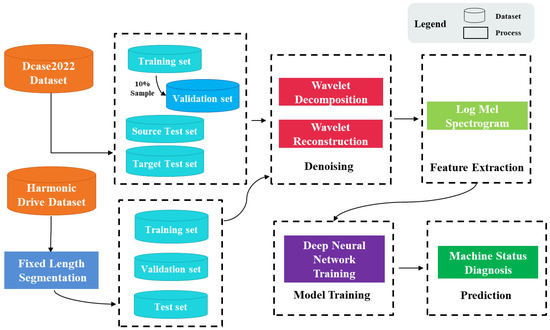
Figure 1. The proposed monitoring model architecture.

For the DCASE 2022 Dataset, data preprocessing was performed first. For each type of machine operating sound sample, the multi-layer Discrete Wavelet Transforms (DWT) were used to remove noise; then, the logarithmic Mel spectrogram was used to extract the features, and finally, the feature data were entered into the deep neural network for training.

For the Harmonic Drive Dataset, each sound sample was cut to increase the number of samples first, and the same process was subsequently applied.

3.2. Dataset

3.2.1. DCASE 2022 Dataset

The DCASE 2022 Dataset is a combination of two datasets, namely the TOYADMOS2 Dataset established by Harada et al. [14] and the MIMII DG Dataset established by Dohi et al. [4]. The TOYADMOS2 Dataset includes sounds of toy trains and toy cars, two different types of industrial machinery, and about 7200 operating sounds recorded under normal and abnormal conditions. The MIMII DG Dataset includes sounds of bearings, fans, gearboxes, slides, and valves. About 18,000 recordings of operating sounds under normal and abnormal conditions were collected from the five different industrial machines.

The TOYADMOS2 Dataset was recorded using a SURE SM11-CN dynamic microphone and a TOMOCA EM-700 condenser microphone. Each sample was of 10 s duration. The team damaged the machine parts and then categorized the damage levels into low, medium, and high levels, finally adding additional factory noises. On the other hand, the sound samples in the TOYADMOS2 Dataset were categorized as the source domain and the target domain. The difference between the two domains lies in the different noise types, signal-to-noise ratios (SNRs), microphone arrangements, and mechanical operating speeds.

The MIMII DG Dataset was recorded using the TAMAGO-03 microphone. Each sample is of 10 s duration. The abnormal types include fan blade damage, gearbox gear damage, valve blockage, etc. Much like the TOYADMOS2 Dataset, the noises of the factory environment were added, and the samples were also categorized as the source domain and the target domain.

3.2.2. Harmonic Drive Dataset

The model of the harmonic drive used in this study was Liming DSF17-100. The recording device was an Adafruit I2S SPH0645 omnidirectional microphone. The microphone performed the recording at 3 cm from the harmonic drives. The recorded 32-bit floating-point audio file with the sample rate was 44,100 Hz, and the SNR was 60 dB (Lin).

The Harmonic Drive Dataset was marked by experts and contained sound files of the same model of machine with different rotation speeds, while the abnormal type only included gear failure. Since the length of each original sample varied, and also to avoid overfitting problems caused by few samples, this research reduced the original sound sample into those with fixed lengths. After cutting a sound file, if the length was less than the specified cutting length, it was discarded. The number of normal and abnormal samples is shown in Table 2 and Table 3.

Table 2. The number of original samples.

	Normal	Abnormal
The number of samples	7	4

Table 3. The number of cutting samples.

	Normal	Abnormal
Number of samples in one second	285	171
Number of samples in three seconds	95	57

3.3. Data Preprocessing

The sound samples may have contained unnecessary sounds, such as environmental noise and factory noise; therefore, the method of separating the sound of machinery from the original samples was an essential step in the monitoring model. In this study, discrete wavelet transforms were used to process sound samples and discard some audio components to remove undesirable noises.

The filter used in this research was the Sym10 wavelet shown in Figure 2, which belongs to the Symlet wavelet family. The Symlet wavelet has the advantage of fast calculation, and is exactly reversible without edge effect problems and memory-saving [15].

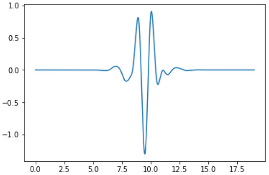
Figure 2. The Sym10 wavelet function.

The process of the wavelet transforms is shown in Figure 3. In the first step, the sample was decomposed into 15-level discrete wavelet decompositions to obtain 15 detail coefficients and 1 approximation coefficient, representing higher frequency audio components and the lowest frequency audio components.

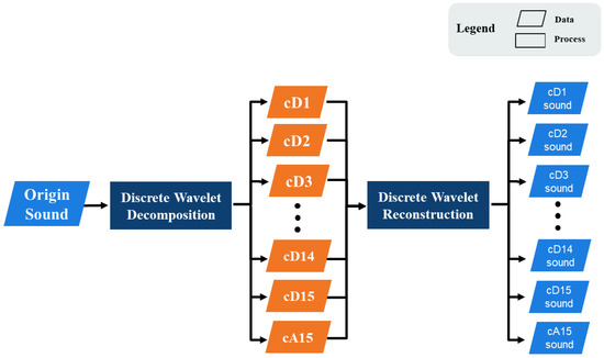
Figure 3. The wavelet transform process.

In the second step, after the wavelet decomposition was completed, the coefficients generated in the previous step were reconstructed through the wavelet reconstruction. The reconstructed sounds were the corresponding audio component of the original sound sample in each frequency interval.

The wavelet decomposition process is shown in Figure 4. For example, considering the two-level one-dimensional wavelet decomposition, the original audio signal X was a one-dimensional input signal, which was passed through a low pass filter g[k] of length K and high pass filter h[k], thus separating the low-frequency and high-frequency components of the signal.

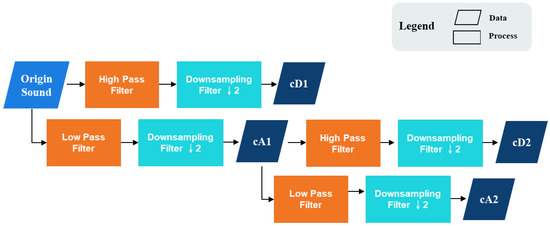
Figure 4. The wavelet decomposition process.

The signal through the down-sampling filter obtained the high-frequency detail coefficient cD1 and the approximate coefficient cA1 of low frequency. Then, cA1 was used as the subsequent input, and the same decomposition steps were performed to obtain the detail coefficient cD2 and the approximate coefficient cA2. The corresponding equations, Equations (3)–(6), are as follows:

This research used 15-level wavelet decomposition to obtain the coefficients set S = {cD1, cD2, cD3, cD4, cD5, cD6, cD7, cD8, cD9, cD10, cD11, cD12, cD13, cD14, cD15, cA15}

$$\mathrm{cD}1\left[n\right]={\displaystyle \sum }_{k=0}^{K-1} \mathrm{X} \left[n+1-k\right]h\left[k\right]$$

(3)

$$\mathrm{cA}1\left[n\right]={\displaystyle \sum }_{k=0}^{K-1} \mathrm{X} \left[n+1-k\right]g\left[k\right]$$

(4)

$$\mathrm{cD}2\left[n\right]={\displaystyle \sum }_{k=0}^{K-1}\mathrm{cA}1\left[n+1-k\right]h\left[k\right]$$

(5)

$$\mathrm{cA}2\left[n\right]={\displaystyle \sum }_{k=0}^{K-1} \mathrm{cA}1\left[n+1-k\right]g\left[k\right]$$

(6)

Since this research only required the audio components of each coefficient, except for the detail coefficients of the audio components slated for reconstruction, the remaining coefficients were replaced by 0 arrays. The audio components were obtained after one or more reconstructions. Taking the cD1 audio component as an example, the 0 arrays and the high-frequency coefficients cD1 were passed through the low-pass reconstruction filter g*[k] and the high-pass reconstruction filter h*[k], respectively, then two signals were added to obtain the cD1 audio component, as shown in Figure 5.

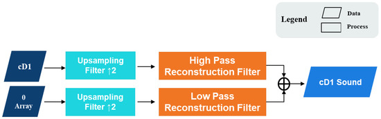
Figure 5. The wavelet reconstruction process.

After obtaining the audio components at each frequency interval, this research adopted different audio components for each machinery type. Removing unnecessary noise improves the prediction performance of the neural network. The audio components selected for each category are shown in Table 4 and Table 5.

Table 4. The audio components selected for machinery type in the DCASE 2022 Dataset.

Type	Audio Components
Toy Car	cD1, cD2, cD3
Toy Train	cD1, cD2, cD3
Bearing	cD1, cD2, cD3, cD4, cD5, cD6, cD7, cD8, cD9, cD10, cD11, cD12, cD13, cD14, cD15, cA15
Fan	cD1, cD2, cD3, cD4, cD5, cD6, cD7, cD8, cD9, cD10, cD11, cD12, cD13, cD14, cD15, cA15
Gearbox	cD1, cD2, cD3
Slide rail	cD1, cD2, cD3
Valve	cD1, cD2, cD3

Table 5. The audio components selected for the Harmonic Drive Dataset.

Type	Audio Components
Harmonic Drive	cD1, cD2

Next, the logarithmic Mel spectrogram was used as the audio feature extraction method, as shown in Figure 6. The sound sample was processed through the short-time Fourier transforms (STFT) shown in Equation (7), the window function w adopted the Hamming window function shown in Equation (8), the STFT frame size was 64 ms, and the frame hop size was 32 ms. The spectrum was obtained after STFT processing.

$$STFT\left\{x\left(n\right)\right\}\left(m,\omega \right)=X\left(m,\omega \right)={\displaystyle \sum }_{n=-\infty }^{\infty }\begin{array}{c}x\left(n\right)w\left(n-m\right)e^{-j\omega n}\end{array}$$

(7)

$$w\left(n\right)=0.5\left(1-\cos \left(\frac{2\pi n}{N-1}\right)\right),0\le n\le N-1$$

(8)

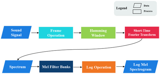
Figure 6. The process of generating the logarithmic Mel spectrogram.

x(n) is the audio with the length of N. The power spectrum can be obtained by squaring the spectrum, as shown in Equation (9), then the power spectrum was processed through 128 Mel filters, and finally, the Power To Decibel (PTB) operation was performed, as in Equation (10), to obtain the Log-Mel-Spectrogram, which was the input data for the deep neural network.

$$Power={\left|X\left(m,\omega \right)\right|}^2$$

(9)

$$PTB\left(S\right)=10\times lo{g}_{10}\left(S\right)$$

(10)

3.4. Deep Neural Network Architecture

The EffienctNetV2S [9] network was used to build the monitoring model. The network architecture is shown in Figure 7. The EffienctNetV2S network was first proposed by Tan et al.; their team used the Fused-MB convolution layer in the early stage of the EffienctNetV2S network and then the MB convolution layer in the later stage to enhance the training efficiency and model performance.

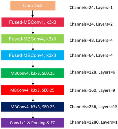
Figure 7. The architecture of the EffienctNetV2S network.

The architecture of Fused-MB convolution and MB convolution are shown in Figure 8 and Figure 9, respectively. The primary difference is whether the neural layer contains the deep-wise convolution structure or the traditional convolution structure.

Figure 8. The architecture of the MB convolution.

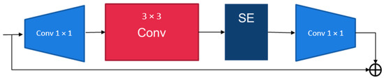
Figure 9. The architecture of the Fused-MB convolution.

In this study, an image of 64 × 128 was the input of the deep neural network, Adam optimizer was used for optimization, and the learning rate was 0.001.

4. Methods

This section introduces the experimental process and results.

4.1. The Experimental Process

For the DCASE 2022 Dataset, this research used the monitoring model constructed by the log Mel-spectrogram, wavelet transforms, and the EfficientNetV2S network to compare with the other two proposed monitoring models. Then, the two Baseline models provided by the organizers of the DCASE 2022 challenge were compared. The hyper-parameters used by the model are shown in Table 6; the mixed precision was used to speed up the computation. The model with the lowest loss in the validation set was saved and examined in the final test phase. Adam was used for optimization in the training phase.

Table 6. Hyperparameters of the monitoring model.

This Paper	DCASE 2022 Dataset	Harmonic Drive Dataset
Training Epochs	200	200
Optimizer	Adam	Adam
Learning Rate	0.001	0.001
Input Image Size	64 × 128	64 × 128
Log Mel Spectrogram Frame Size	1024	1024
Batch Size	128	16

For the Harmonic Drive Dataset, the monitoring model with the best performance in the DCASE 2022 Dataset experiment was used as the anomaly monitoring model of the harmonic drive. The test process was the same as the above-described process.

4.2. The Experimental Results

The harmonic drive is a type of gearbox, so the gearbox audio samples could be used to evaluate the anomaly detection model for the harmonic drive. For the sample source of the gearbox, the DCASE 2022 Dataset Gearbox audio samples were used.

The model with the highest AUC was selected by comparison through experiments. Three models were proposed in this study for gearbox machinery anomaly detection. The AUC of the three models is shown in Table 7. Model one, which combined logarithmic Mel spectrogram, wavelet transforms, and the EfficientNetV2S network architecture, achieved the best prediction performance. Thus, this research used model 1 for subsequent comparisons with methods proposed in other studies.

Table 7. The performance of the proposed gearbox anomaly detection models.

	Model 1 Log Mel Spectrogram + Wavelet Transforms + EfficientNetV2S		Model 2 Log Mel Spectrogram + EfficientNetV2S		Model 3 Log Mel Spectrogram + Wavelet Transforms + MobileNetV2
	Source_test	Target_Test	Source_Test	Target_Test	Source_Test	Target_Test
ID_01	0.7176	0.6804	0.6968	0.7032	0.6484	0.6884
ID_02	0.7992	0.7579	0.67	0.6291	0.6554	0.5802
ID_03	0.8573	0.5222	0.8384	0.4454	0.717	0.6452
Average	0.7914	0.6535	0.7351	0.5926	0.6736	0.6379
Average of two domains	0.7224		0.6638		0.6558

The proposed model outcomes were compared with those of two baseline models provided by the organizers of the DCASE 2022 Challenge. The results presented in Table 8 show that the average AUC of the proposed model was about 6% higher than those of the two baseline models, suggesting that the proposed model performed better than the two baseline models for gearbox anomaly detection tasks in real factory scenarios.

Table 8. Comparison with other studies on gearbox samples.

	This Paper		Log Mel Spectrogram + AutoEncoder [4]		Log Mel Spectrogram + MobileNetV2 [4]
Gearbox	Source_Test	Target_Test	Source_Test	Target_Test	Source_Test	Target_Test
ID_01	0.7176	0.6804	0.6463	0.6479	0.6354	0.6702
ID_02	0.7992	0.7579	0.6766	0.5812	0.6668	0.6696
ID_03	0.8573	0.5222	0.7538	0.6557	0.8087	0.4315
Average	0.7914	0.6535	0.6922	0.6283	0.7037	0.5904
Average of two domains	0.7224		0.6603		0.6471

Further, the model’s performance in fault detection tasks was examined for various types of machinery in the DCASE2022 Dataset to assess whether the proposed model could detect general machinery anomalies. The results in Table 9 suggest a good capability of the proposed model for the detection of various types of machinery anomalies. The overall AUC was 5% higher than that of baseline models on average, and the AUC of the Slider category was nearly 20% higher.

Table 9. Comparison with other papers when using the DCASE 2022 Dataset.

	This Paper		Log Mel Spectrogram + AutoEncoder [4]		Log Mel Spectrogram + MobileNetV2 [4]
	Source_Test	Target_Test	Source_Test	Target_Test	Source_Test	Target_Test
Toycar	0.678	0.6713	0.917	0.3664	0.6121	0.5281
Toytrain	0.6835	0.4339	0.7698	0.2636	0.604	0.463
Bearing	0.6309	0.5609	0.5695	0.5901	0.6307	0.6179
Fan	0.58	0.5487	0.7897	0.4919	0.7154	0.5176
Gearbox	0.7914	0.6535	0.6922	0.6283	0.7037	0.5904
Slider	0.9539	0.7175	0.7881	0.4904	0.6984	0.4859
Valve	0.6483	0.603	0.5209	0.4986	0.6877	0.6092
Average	0.7094	0.5984	0.7210	0.4756	0.6646	0.5446
Average of two domains	0.6539		0.5983		0.6046

After the proposed model was evaluated on the DCASE 2022 Dataset, the Log Mel spectrogram, discrete wavelet transforms, and EffientNetV2S network were used to build the harmonic drive anomaly monitoring model. As the training set of the experiment, we randomly selected 60% of the data from the normal samples and abnormal samples of the Harmonic Drive Dataset and considered 20% of the data as the validation set; the remaining 20% of the data was used as the test set.

In this research, samples of 1 s duration were used for the experiments. The proposed model was compared with other models for rotating machinery anomaly sound detection, including the method that uses the Fast Kurtogram combined with deep convolution to predict bearing anomalies proposed by Prosvirin et al. [16] and our previous research [17] that uses the wavelet transforms combined with the fully connected network to predict the wind turbine blade anomalies. The results are shown in Table 10.

Table 10. Comparison of the proposed model with other models when using the Harmonic Drive Dataset.

	Accuracy	AUC
This paper	0.901	0.9302
Prosvirin et al. [16]	0.91	0.911
Kuo et al. [17]	0.858	0.89

This research explored the impact of sample duration and noise on prediction performance. Based on duration, the samples were categorized into one second and three seconds.

The results of the prediction accuracy of different sample durations are shown in Table 11. The prediction AUC of the monitoring model for the three-second category was lower than that for the one-second category, possibly because the model needs a larger number of samples to detect the pattern of the anomaly sounds.

Table 11. The experiment results of different sample durations.

	AUC
Samples with a 1-s duration	0.9302
Samples with a 3-s duration	0.881

Regarding the noise, additive white Gaussian noise was added to the 1 s duration sound samples. The two kinds of SNRs for the experiments were of the 20 dB(Lin) and 10 dB(Lin) categories. The prediction AUC results with different SNRs in this research are shown in Table 12.

Table 12. The experiment results of different SNRs.

	AUC
Samples without adding noise	0.9302
SNR = 20 dB (Lin)	0.87
SNR = 10 dB (Lin)	0.86

Table 12 shows that the intensities of noise and the prediction AUC results of the model are related. In the case of noise addition, the model could still maintain a good prediction performance, indicating that the proposed mode has noise processing ability and can perform the anomaly detection task of the harmonic drive even in the presence of background noise.

5. Conclusions

This research proposes a harmonic drive anomaly detection model by combining discrete wavelet transforms, the Log Mel spectrogram, and the EffientNetV2S network architecture. The model uses wavelet transforms to separate the original sample audio into audio components representing each frequency interval, then uses the Log Mel spectrogram to extract features, and finally enters features as inputs into the neural network for training. The detection model exhibited an excellent prediction performance for the DCASE 2022 Dataset and the Harmonic Drive Dataset.

The proposed detection model uses only the sound of mechanical operation as the anomaly judgment. If data such as vibration information or thermal energy are added to the model, the prediction performance of the model may be further improved.

The parameter settings of the denoise algorithm were adjusted manually, and the best combination was compared through experiments. The audio pre-processing efficiency may be improved if the optimization algorithm is used to adjust each parameter, thus further enhancing the prediction capability.

References

- Yang, G.; Zhong, Y.; Yang, L.; Du, R. Fault Detection of Harmonic Drive Using Multiscale Convolutional Neural Network. IEEE Trans. Instrum. Meas. 2020, 70, 1–11. [Google Scholar] [CrossRef]
- Meng, H.; Yan, T.; Yuan, F.; Wei, H. Speech Emotion Recognition From 3D Log-Mel Spectrograms With Deep Learning Network. IEEE Access 2019, 7, 125868–125881. [Google Scholar] [CrossRef]
- Oo, M.M.; Oo, L.L. Fusion of Log-Mel Spectrogram and GLCM Feature in Acoustic Scene Classification. In Software Engineering Research, Management and Applications; Springer: Cham, Switzerland, 2019; pp. 175–187. [Google Scholar] [CrossRef]
- Dohi, K.; Nishida, T.; Purohit, H.; Tanabe, R.; Endo, T.; Yamamoto, M.; Kawaguchi, Y. MIMII DG: Sound Dataset for Malfunctioning Industrial Machine Investigation and Inspection for Domain Generalization Task. arXiv preprint 2022, arXiv:2205.13879. [Google Scholar]
- Zagoruyko, S.; Komodakis, N. Wide residual networks. arXiv preprint 2016, arXiv:1605.07146. [Google Scholar]
- He, K.; Zhang, X.; Ren, S.; Sun, J. Deep residual learning for image recognition. In Proceedings of the IEEE conference on computer vision and pattern recognition, Las Vegas, NV, USA, 27–30 June 2016; pp. 770–778. [Google Scholar]
- Tan, M.; Chen, B.; Pang, R.; Vasudevan, V.; Sandler, M.; Howard, A.; Le, Q.V. Mnasnet: Platform-aware neural architecture search for mobile. In Proceedings of the IEEE/CVF Conference on Computer Vision and Pattern Recognition, Long Beach, CA, USA, 15–20 June 2019; pp. 2820–2828. [Google Scholar]
- Russakovsky, O.; Deng, J.; Su, H.; Krause, J.; Satheesh, S.; Ma, S.; Fei-Fei, L. Imagenet large scale visual recognition challenge. Int. J. Comput. Vis. 2015, 115, 211–252. [Google Scholar] [CrossRef]
- Tan, M.; Le, Q. Efficientnetv2: Smaller models and faster training. In Proceedings of the International Conference on Machine Learning, PMLR, online, 13–14 August 2021; pp. 10096–10106. [Google Scholar]
- Chen, W.; Li, J.; Wang, Q.; Han, K. Fault feature extraction and diagnosis of rolling bearings based on wavelet thresholding denoising with CEEMDAN energy entropy and PSO-LSSVM. Measurement 2020, 172, 108901. [Google Scholar] [CrossRef]
- Zhi, Z.; Liu, L.; Liu, D.; Hu, C. Fault Detection of the Harmonic Reducer Based on CNN-LSTM With a Novel Denoising Algorithm. IEEE Sensors J. 2021, 22, 2572–2581. [Google Scholar] [CrossRef]
- Sahoo, S.; Kushwah, K.; Sunaniya, A.K. Health Monitoring of Wind Turbine Blades through Vibration Signal Using Advanced Signal Processing Techniques. In Proceedings of the 2020 Advanced Communication Technologies and Signal Processing (ACTS), Silchar, India, 4–6 December 2020; pp. 1–6. [Google Scholar] [CrossRef]
- Dcase Challenge 2022—Unsupervised Anomalous Sound Detection for Machine Condition Monitoring Applying Domain Generalization Techniques. Available online: https://dcase.community/challenge2022/task-unsupervised-anomalous-sound-detection-for-machine-condition-monitoring (accessed on 31 May 2022).
- Harada, N.; Niizumi, D.; Takeuchi, D.; Ohishi, Y.; Yasuda, M.; Saito, S. ToyADMOS2: Another dataset of miniature-machine operating sounds for anomalous sound detection under domain shift conditions. arXiv preprint 2021, arXiv:2106.02369. [Google Scholar]
- Yadav, A.K.; Roy, R.; Kumar, A.P.; Kumar, C.S.; Dhakad, S.K. De-noising of ultrasound image using discrete wavelet transform by symlet wavelet and filters. In Proceedings of the 2015 International Conference on Advances in Computing, Communications and Informatics (ICACCI), Kochi, India, 10–13 August 2015; pp. 1204–1208. [Google Scholar] [CrossRef]
- Prosvirin, A.; Kim, J.; Kim, J.M. Bearing fault diagnosis based on convolutional neural networks with kurtogram representation of acoustic emission signals. In Advances in Computer Science and Ubiquitous Computing; Springer: Singapore, 2017; pp. 21–26. [Google Scholar]
- Kuo, J.-Y.; You, S.-Y.; Lin, H.-C.; Hsu, C.-Y.; Lei, B. Constructing Condition Monitoring Model of Wind Turbine Blades. Mathematics 2022, 10, 972. [Google Scholar] [CrossRef]
Publisher’s Note: MDPI stays neutral with regard to jurisdictional claims in published maps and institutional affiliations. |
© 2022 by the authors. Licensee MDPI, Basel, Switzerland. This article is an open access article distributed under the terms and conditions of the Creative Commons Attribution (CC BY) license (https://creativecommons.org/licenses/by/4.0/).