A Forwarding Latency Optimization Method for Software Data Plane Based on Spin-Polling

Abstract

Modern software data planes use spin-polling and batch processing mechanisms to significantly improve maximum throughput and forwarding latency. The user-level IO queue-based spin polling mechanism has a higher response speed than the traditional interrupt mechanism. The batch mechanism enables the software data plane to achieve higher throughput by amortizing the IO overhead over multiple packets. However, the software data plane under the spin-polling mechanism keeps running at full speed regardless of the input traffic rate, resulting in significant performance waste. At the same time, we find that the batch processing mechanism does not cope well with different input traffic, mainly reflected in the forwarding latency. The purpose of this paper is to optimize the forwarding latency by leveraging the wasted performance. We propose a forwarding latency optimization scheme for the software data plane based on the spin polling mechanism in this paper. First, we calculate the CPU utilization of the software data plane according to the number of cycles the CPU spends on the valuable task. Then, our scheme controls the Tx queues and dynamically adjusts the output batch size based on the CPU utilization to optimize the forwarding latency of the software data plane. Compared with the original software data plane, the evaluation result shows that the forwarding latency can be reduced by 3.56% to 45% (in a single queue evaluation) and 4.35% to 55.54% (in a multiple queue evaluation).

1. Introduction

Software data planes have a wide range of applications in many fields, such as high-speed packet processing [1], software-defined networking (SDN) [2,3,4], network function virtualization (NFV) [5], and I/O virtualization [6]. The traditional kernel IO stack relies on system interrupts and system calls, and its response speed is no longer able to meet the increasing performance requirements of the software data plane. Many modern software data planes have taken a series of measures and mechanisms to achieve fast notification mechanisms and low-overhead operations in order to achieve low latency and high throughput. These mechanisms and measures are mainly the following three: (1) Kernel bypass [7,8,9,10,11]. The response speed of the traditional kernel IO stack has lagged too far behind, and the software data plane needs more user-level IO capability support, including user-level queues, user-level storage frameworks, and so on. (2) Spin-polling [12,13,14,15,16,17,18]. The spin-polling mechanism is one of the key designs for low-latency software data planes. CPU cores that execute the poll loop at high speed have the property of fast-reacting with low overhead because they do not block or wait, and the cores can spin locally in their cache when there is no work [6]. (3) Batch processing [19,20,21]. The batch processing mechanism can better handle high input traffic because it amortizes the IO overhead over multiple packets, which reduces the average overhead per packet, thus improving the packet processing capacity of the software data plane [19,22,23].

Despite bringing considerable performance gains to the software data plane, the spin-polling and batch processing mechanisms still have some problems. First, a feature of the spin-polling mechanism is that the spinning cores always run full-tilt, which means that when the load of the software data plane is low, the spinning cores are still running full-tilt [6]. In other words, the spinning cores have a high percentage of useless work at low loads. In addition, this poses the problem of not being energy efficient [24]. Second, the batch processing mechanism is also ineffective at coping with low-load scenarios. Miao et al. found that packets wait in the user-level Rx queues until the length of the Rx queues reaches the Rx batch size [19], which increases the forwarding latency of the software data plane. The above two issues inspire us to focus on the performance of the software data plane at a low load and the behavior of the Rx/Tx queues.

In this paper, we focus on the forwarding latency of the software data plane and propose a forwarding latency optimization scheme based on the dynamic adjustment of the Tx batch size. The main contributions of this paper are as follows:

• We conduct a series of experiments, and the experimental results show that the forwarding latency of the software data plane has a specific relationship with the system load and the batch size of the batch processing mechanism. The batch size is not always the larger, the better.
• We analyze the characteristics of the forwarding latency of the software data plane based on spin-polling at different loads by a simple model.
• We propose a forwarding latency optimization scheme for the software data plane based on the spin-polling mechanism. First, we calculate the CPU utilization of the software data plane according to the number of cycles the CPU spends on the valuable task. Then, based on the CPU utilization calculated in real-time, the scheme optimizes the forwarding latency of the software data plane at different loads by controlling the Tx queues and dynamically adjusting the Tx batch size.
• We build a primary software data plane using Data Plane Development Kit (DPDK) on a Dell R740 server and implemented our proposed scheme on it. In addition, we give a detailed evaluation of our scheme, including a comparison with the original software data plane and Smart Batching [19].

The structure of this paper is organized as follows. In Section 2, we detail the related work, including the software data plane architecture, the spin-polling mechanism, and the batch processing mechanism. We perform some experiments and use the experimental results to illustrate the motivation of our work in Section 3. In Section 4, we illustrate the experimental results of Section 3 with a simple model and lead to the starting point of our scheme. We present our latency optimize scheme based on the dynamic adjustment of Tx batch size in Section 5, and the details of scheme implementation are performed in Section 6. Finally, we conclude this paper and discuss the future works in Section 7.

2. Related Work

In this section, we introduce the basic architecture of software data planes, and the details of the spin-polling mechanism and batching mechanism.

2.1. Software Data Plane

In software-defined networking (SDN) and network functions virtualization (NFV), software data planes play one of the crucial roles. Compared with traditional high-coupling network data plane facilities, software data planes can provide higher flexibility and programmability to meet more application requirements [25,26,27]. Software data planes in the SDN field can provide more packet operations, such as modification, insertion, and deletion of packet headers. In addition, unlike traditional devices, software data planes use multiple layers of headers, including but not limited to Layer 2 to Layer 5.

Software data planes based on kernel IO stacks have been stretched to the limit in terms of performance. Many modern software data planes improve performance by bypassing the kernel IO stack, enabling cores to poll on user-level queues, and applying batch processing mechanisms. To reduce system calls or interrupts, using user-level IO to bypass the kernel IO stack is a classic approach. There is a lot of previous work on user-level IO capabilities, such as user-level networking stacks (mTCP [9], Sandstorm [8], MICA [7], and eRPC [10]), user-level storage frameworks (NVMeDirect [28], SPDK Vhost-NVMe [29]), and direct access to virtualized IO (Arrakis [11]), to name a few.

Software data planes running on an x86 server can access a set of logical CPU cores and a set of physical or logical ports. Modern network interface controllers (NICs) support hardware multiple Rx/Txqueues. Some NIC technologies, such as Receive Side Scaling (RSS), can distribute packets from the same link to multiple different hardware Rx queues by hashing the packet’s header. The data planes can bind different logical CPU cores to hardware Rx queues and Tx queues, respectively. Therefore, several logical CPU cores can efficiently process the packets from the same link in parallel [30]. Figure 1 shows the basic architecture of the software data plane with M NIC ports and N CPU cores for packet processing. In the architecture shown in Figure 1, each NIC port of the data plane is configured with N Rx queues and Tx queues, corresponding to N logical CPU cores for packet processing. Therefore, each logical CPU core needs to process packets from M Rx queues, and it can forward packets to M Tx queues. In addition, each logical CPU core is independent of the other and does not need to compete for packets, so there are no synchronization and locking issues in packet processing. Therefore, we can focus only on a single logical CPU core and its bound Rx/Tx queues.

Figure 1. The basic architecture of software data plane.

2.2. Spin-Polling Mechanism

The traditional network stack processes packets based on an interrupt mechanism. The NIC will generate a hardware-level interrupt signal whenever a packet arrives to notify the CPU. After the CPU receives an interrupt signal, it will copy the packets from the direct memory access (DMA) memory area to the kernel mbuff structures at an appropriate time. This mechanism seems to be acceptable in scenarios with low network traffic load [12]. However, when the network traffic load becomes heavy, the interrupt mechanism will generate too many interrupt signals, and the generation, transmission, and processing of these signals will cause much overhead [19]. These excessive overheads make traditional network stacks unable to cope with ever-increasing traffic rates.

In order to cope with the pressure of high network traffic load, modern high performance network packet processing frameworks, such as PacketShader [31], netmap [32], DPDK [1], etc., mainly rely on the spin-polling mechanism and user-level NIC queues to speed up the processing of packets. Moreover, many modern software data planes, such as Shenango [14], Shinjuku [15], Andromeda [16], IX [12], and ZygOS [13], are all based on the spin-polling mechanism. The characteristic of the spin-polling mechanism is that the CPU cores will continuously and actively check whether new packets arrive. As mentioned earlier, in the software data plane architecture, the CPU core must process packets from multiple Rx queues to which it is bound. Therefore, a CPU core under the spin-polling mechanism polls the Rx queues bound to it in a particular order (e.g., in a round-robin fashion). As shown in Figure 2, the CPU core will check whether there are new packets in each Rx queue in a round-robin fashion. Once the CPU core receives new packets from an Rx queue, it will process them instead of continuing to check the next Rx queue. If these packets are not dropped, they are either put into the Tx queues for forwarding or sent to the controller after processing. Then, the CPU core will continue to check the next Rx queue.

Figure 2. Schematic diagram of a single CPU working based on the spin-polling mechanism.

Typically, CPU cores are polling at high speed on user-level queues, providing faster responsiveness and controllability than traditional IO stacks that rely on interrupt notification capabilities. Although spinning cores design is the key design idea of many low-latency software data planes, it also brings the problem of non-energy saving and wasted processing capability [6]. Under the spin-polling mechanism, the CPU core is always running full-tilt even if there are no packets in the Rx queues. Therefore, there is not always valuable work for the CPU core. Some high-speed data plane processing frameworks provide a hybrid interrupt polling model, such as the l3fwd-power example provided by DPDK, which aims to solve the problem of non-energy saving at the expense of packet processing capability and latency.

2.3. Batch Processing Mechanism

The batch processing mechanism are widely used on high-speed data plane processing frameworks, such as Netmap [32], PacketShader [31], DPDK [1], PF_RING [33], Open Onload [34], and PACKET_MMAP [35], and is usually combined with the spin-polling mechanism. The core of the batch processing mechanism is to amortize the fixed overhead over multiple packets. Batch processing has the advantages of improved instruction cache locality, prefetching effectiveness, and the prediction accuracy [22]. There is also a lot of previous work studying batch mechanisms. Ref. [30] proposes a performance evaluation model by analyzing software virtual switches based on batch mechanisms. Ref. [20] proposes a generic model that allows for detailed prediction of performance metrics related to NFV routers based on batch mechanisms. Ref. [19] focuses on a high-speed data plane processing framework for Rx batch size, and proposes a load-sensitive dynamic adjustment method of Rx batch size to reduce the packet latency.

Unless otherwise specified, the length of the Rx/Tx queues in this paper refers to the number of packets in the Rx/Tx queues. In the software data plane, there is a batch size in both the Rx queue and the Tx queue, which we call the Rx batch size ${\theta }_{Rx}$ and the Tx batch size ${\theta }_{Tx}$, respectively. Specifically, the ${\theta }_{Rx}$ is an “upper limit”: it specifies the upper limit of the number of packets that can be received each time the CPU core checks one Rx queue. However, the ${\theta }_{Tx}$ is a “threshold”: if the length of a Tx queue reaches the threshold, all the packets in the queue will be sent out, which we call regular burst mode; otherwise, the packets will wait in the queue. Note that the data plane cannot tolerate packets staying in the Tx queue for too long. When the network load is light, the length of the Tx queue often takes a long time to reach the threshold ${\theta }_{Tx}$. In order to cope with the light network load, a timer or a counter can limit the waiting time of the packets in the Tx queues. In fact, maintaining a timer costs more than a counter. The latter sets a threshold N of polling times for a CPU core. When the CPU core polls N times, it will perform a Tx queue flushing: forwarding all packets in all Tx queues, which we call timeout flush mode.

Many existing works [12,13,14,15,16] only focus on the benefits of fast notifications brought by the spin-polling mechanism, while ignoring the performance waste caused by the spinning cores. Ref. [6] raises the problem of performance waste under the spin-polling mechanism and explores the queue scalability under this mechanism, but they do not give performance optimization suggestions in combination with the batch processing mechanism. In terms of the batch processing mechanism, some works [20,30] are limited to the performance model analysis under this mechanism. Ref. [19] notes that some adjustments to the batch processing mechanism could improve forwarding latency, but the study only focuses on Rx queues, and the analysis is limited. Our work focuses on the spin-polling mechanism, and by analyzing the characteristics of the data plane under different input traffic rates, we propose a batch processing mechanism adjustment method relying on real-time CPU utilization, which can effectively improve the forwarding latency of the data plane at different input traffic rates.

3. Motivation

In this section, we first analyze the advantages and disadvantages of the spin-polling mechanism and batch processing mechanism. Then, we use some experiments to explore the characteristics of the forwarding latency and throughput of the software data plane under these mechanisms.

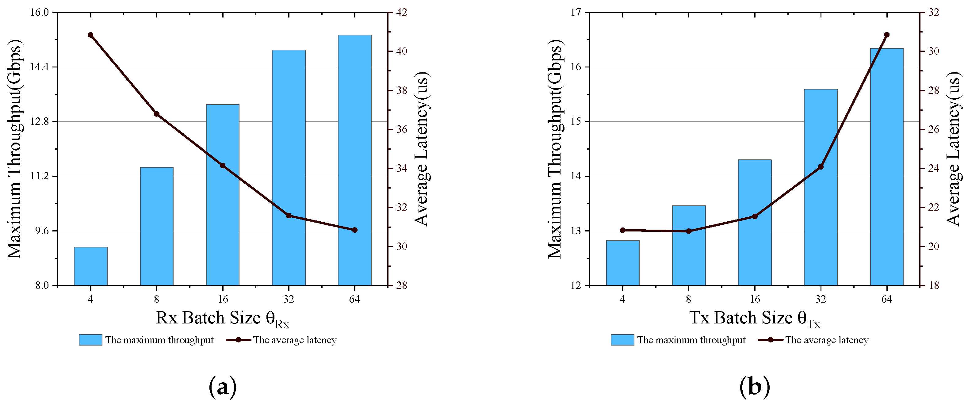
3.1. Static Batch Size

The ${\theta }_{Rx}$ and ${\theta }_{Tx}$ are usually configured as startup parameters and are therefore static parameters during program execution. Therefore, this section discusses the premise that ${\theta }_{Rx}$ and ${\theta }_{Tx}$ are fixed values unless otherwise specified.

As mentioned earlier, ${\theta }_{Rx}$ is an upper limit value, and ${\theta }_{Tx}$ is a threshold value. The difference in the definitions of ${\theta }_{Rx}$ and ${\theta }_{Tx}$ determines the behavior of the CPU core on the Rx queues and the Tx queues. To understand the effect of these two batch sizes on the data plane, we first start with data plane performance metrics. Regarding performance indicators, we generally focus on the maximum throughput of the data plane and the forwarding latency. The maximum throughput of the data plane generally refers to the maximum number of packets per second that can be transmitted without any error. The forwarding latency generally refers to the time required for a packet to travel from the originating device through the data plane to the destination device. Note that each CPU core has a limited number of cycles per second, so the fewer the cycles it takes to process a packet on average, the higher the throughput. When the traffic load is heavy, the CPU core has a high probability of directly receiving ${\theta }_{Rx}$ packets each time it checks an Rx queue. Meanwhile, the number of packets in the Tx queues has a high probability of reaching ${\theta }_{Tx}$. Therefore, in the case of heavy traffic load, the batch processing mechanisms can reduce the amortized overhead of a single packet, allowing the data plane to achieve high throughput performance.

On the other hand, when the traffic load is not so heavy (for example, below 90% load), the number of packets in the queues is likely to be less than ${\theta }_{Rx}$ each time the CPU core checks the Rx queues. However, the CPU core will still receive and process these packets, although doing so will increase the amortized overhead. Note that in a spin-polling system, the CPU cores always run full-tilt regardless of the traffic load. Therefore, the packet processing performance of the spin-polling system is excessive in the case of a low traffic load. From this point of view, the increased overhead is a reasonable use of CPU resources. At the same time, the CPU cores process and forward the packets in the Rx queues in time, which can prevent the packets from staying on the data plane device for a longer time. When the traffic load is light for Tx queues, the probability of the number of packets in the queues reaching ${\theta }_{Tx}$ is not high, so the packets need to wait in the queues. We mentioned earlier that the batch processing mechanism uses a counter to deal with this situation. Nevertheless, we still notice that the existing batch processing mechanism cannot perfectly cope with different traffic input rates, mainly reflected in the forwarding latency of the software data plane. In the next section, we design experiments to investigate the effect of batch processing mechanisms on the performance of the software data planes.

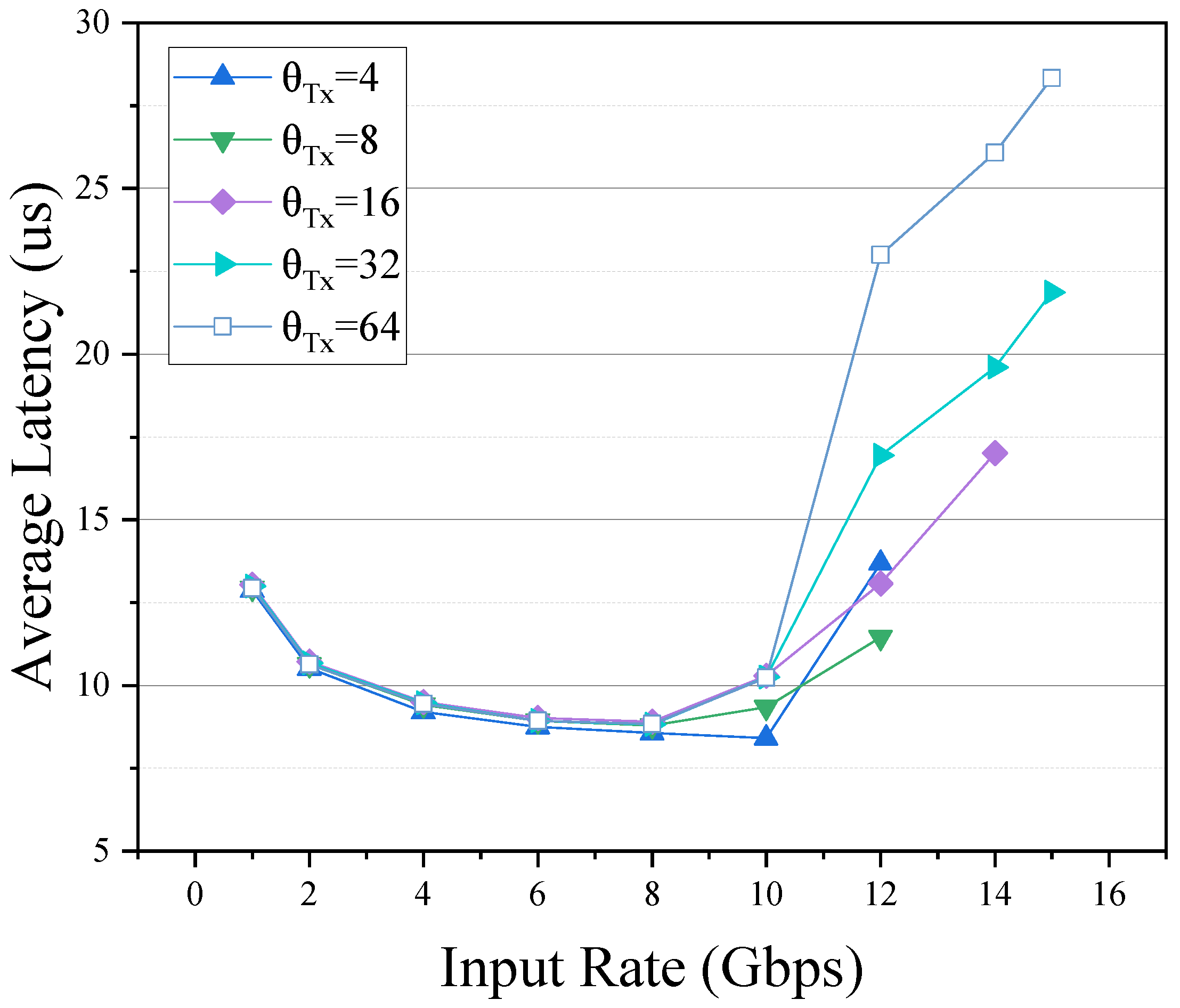
3.2. The Effects of Batch Processing Mechanisms

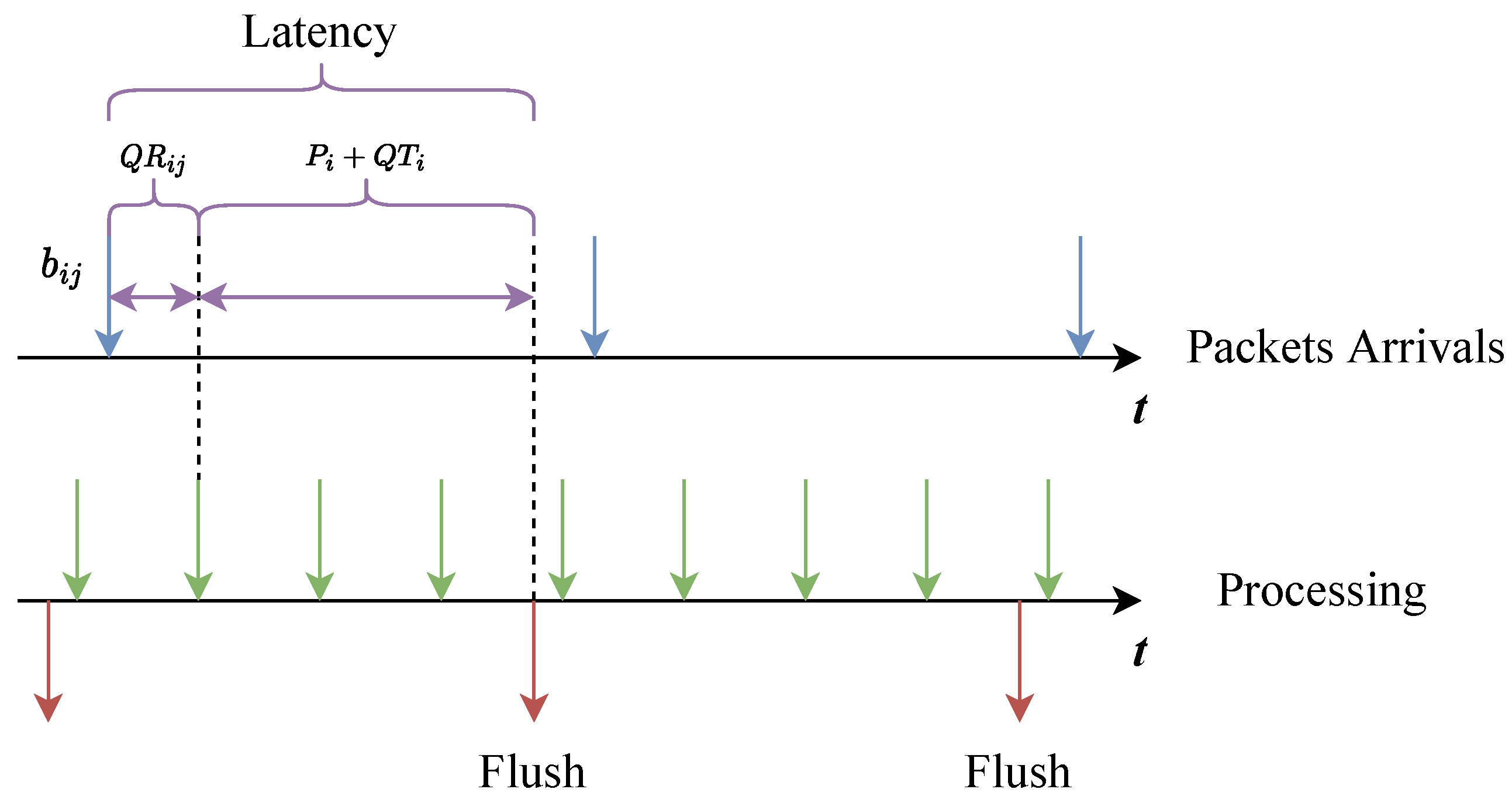
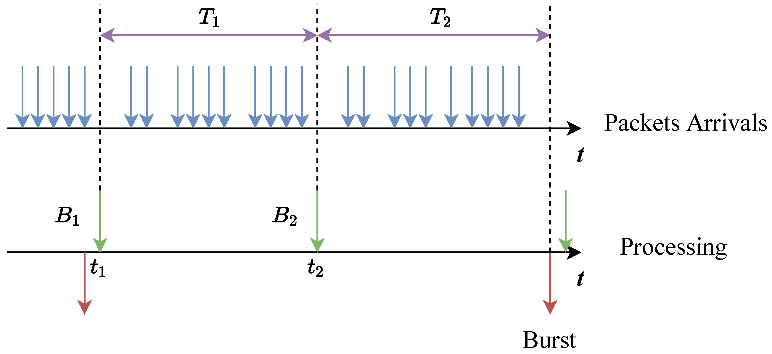
In this section, we use DPDK, a high-performance IO framework with classic spin-polling architecture, to build our experimental environment. DPDK provides an ip_pipeline application, an excellent base case that can be used to implement SDN software switch. We implemented an L4 forwarding application based on the ip_pipeline as a test program for this paper.The testbed is shown in Figure 3a. Our software data plane is deployed in a Dell R740 server with an Intel E810 NIC that provides a maximum data rate of 100 Gbps, and we configure the NIC to 4 × 25 Gbps mode. The NIC receives traffic from an Ixia XGS12 network test platform, a separate packet generator connected to the NIC ports. The detailed experimental configuration is shown in Table 1. The queue configuration is shown in Figure 3b.

Figure 3. The experimental configurations. (a) The testbed topology. (b) The queue configuration.

Table 1. The Detailed Experimental Configurations.

Environment	Information
CPU	Intel Xeon Silver 4216 CPU @2.10 GHz
NIC	Intel Ethernet Connection E810 Series
DPDK Version	21.11.1(LTS)
Ixia Network Version	8.30

We experiment with one CPU core, one Rx queue and one Tx queue to explore the effect of the batch processing mechanism. We use 512-byte fixed-length IPv6 TCP packets for experiments, and some flow tables and flow entries are installed on the data plane to support packet forwarding.

First, we rewrite part of the code of DPDK to collect the performance parameters of the data plane under different ${\theta }_{Rx}$ and ${\theta }_{Tx}$. Then, we use the control variables method to explore the effect of ${\theta }_{Tx}$ and ${\theta }_{Rx}$ on the performance of the data plane respectively. We fix ${\theta }_{Tx}$ to 64 and collect the performance parameters for ${\theta }_{Rx}$ = 4, 8, 16, 32, and 64, as shown in Figure 4a. Similarly, we fix ${\theta }_{Rx}$ to 64 and collect the performance parameters for ${\theta }_{Tx}$ = 4, 8, 16, 32, and 64, as shown in Figure 4b. It is clear that the maximum throughput of the data plane increase with the two batch size. This result is consistent with the analysis above and also reflects the advantages of the batch processing mechanism. At the same time, we also observe that the average latency increases with increasing ${\theta }_{Tx}$ and decreases with increasing ${\theta }_{Rx}$.

Figure 4. The performance of data plane with different Batch Size. (a) ${\theta }_{Tx}=64$. (b) ${\theta }_{Rx}=64$.

Figure 5 shows the average latency of packets forwarded through the data plane under different input rates. For simplicity, we denote the average latency curve in Figure 5 by $T_{{\theta }_{Tx}}\left(r\right)$. When the traffic rate r is in the range [1, 8] Gbps, $T_{{\theta }_{Tx}@8}\left(r\right)$, $T_{{\theta }_{Tx}@16}\left(r\right)$, $T_{{\theta }_{Tx}@32}\left(r\right)$, and $T_{{\theta }_{Tx}@64}\left(r\right)$ almost overlap, so the ${\theta }_{Tx}$ has little effect on the average latency of packets in this rate range. At the same time, we noticed that, in this range, the average latency of packets decreases with rate r. When r is in the range [10, 15] Gbps, the average latency of packets increase with the ${\theta }_{Tx}$. Moreover, in the range [8, 15] Gbps, the average latency of packets increases with rate r.

Figure 5. The average latency under different input rates and different ${\theta }_{Tx}$.

From the above experiments, we can conclude that in the spin-polling system, unlike ${\theta }_{Rx}$, ${\theta }_{Tx}$ is not always the larger, the better. The average latency is related to the size of ${\theta }_{Tx}$, which motivates us to look for a mechanism to adjust ${\theta }_{Tx}$ to optimize the average latency of packets dynamically.

4. Model Analysis

In this section, we qualitatively analyze the experimental results in Section 3.2 through a simple model. Our model is based on a single Rx queue, but the conclusions can be easily generalized to scenarios with multiple Rx queues. The analysis in this section also inspires us to propose an optimization method to optimize the packet latency of the data plane based on the spin-polling system and the batch mechanism. Note that the experiments in Section 3.2 use fixed-length packets, so when we discuss the experimental results in Section 3.2, we do not need to distinguish between the packet arrival rate and the traffic arrival rate. However, in actual scenarios, since the packet lengths cannot be the same, the packet arrival and the traffic arrival rates cannot be confused. Table 2 represents the main notations used in this section.

Table 2. Summary of Notations.

Notation	Description
$b_i$	The number of packets in small batch
$t_i$	The time interval between $b_i$ and $b_{i+1}$
$B_i$	The number of packets received by the CPU at one time
m	The number of times the CPU receives packets between packets forwarding
N	The polling counter threshold
$RT$	The residence time of packets on the data plane
P	The time taken by CPUs to process packets
$QT$	The queuing time of packets in Tx queues
$QR$	The queuing time of packets in Rx queues
$\tau$	The time interval for CPU polling when no packets arrive

The packet arrivals can be regarded as a batch arrival process, as shown in Figure 6. The packet arrivals can be described by a sequence $\{\cdots ,(b_{j-1},t_{j-1}), (b_j,t_j),(b_{j+1},t_{j+1}),\cdots \}$, where $b_j(b_j\in {\mathbb{Z}}^{+})$ represents the number of packet in this batch and $t_j(t_j>0)$ is the time interval between this batch and next batch of packets. The available data buffer addresses are stored in the Rx queues. When the packets arrive at the port, the NIC will write them to the memories where the data buffer addresses point to. The CPUs do not participate in this procedure and therefore do not wait for the packets to be written to memories.

Figure 6. Schematic diagram of packets arrival in batches.

We assume that the CPU checks the Rx queues m times between packets forwarding, and the number of packets received is $B_1,B_2,\cdots ,B_m$, and $B_i$ satisfies the following formula:

$$B_i=\sum _{j=1}^n{b}_{ij},b_{ij}\in {\mathbb{Z}}^{+}\mathrm{when}{B}_i\ne 0(1⩽i⩽m)$$

(1)

where $b_{ij}$ is the j-th small batch packets of $B_i$. Formula (1) means that if the number of packets polled by the CPU is not equal to 0, then these packets are composed of multiple small batches. The residence time $RT$ of the $b_{ij}$’s packets in the data plane can be expressed by the following formula:

$$R{T}_{ij}=Q{R}_{ij}+P_i+Q{T}_i$$

(2)

where $Q{R}_{ij}$ is the queuing time of $b_{ij}$’s packets in Rx queues, $Q{T}_i$ is the queuing time of $B_i$’s packets in Tx queues and $P_i$ is the time taken by CPUs to process $B_i$’s packets.

As mentioned in Section 2.3, there are two packet forwarding modes in the data plane: regular burst mode and timeout flush mode. The data plane will mainly use the timeout flush mode when the packet arrival rate is low, and the regular burst mode will be the primary mode when the packet arrival rate is high. Assuming that N is the polling counter threshold, $\tau$ is the time interval for CPU polling when no packets arrive, which means that: when $B_i=0,P_i=\tau$.

Now we consider the case where the packet arrival rate is very low. In this case, we have $m=N$, and we reasonably assume that ${\sum }_{i=1}^m{B}_i\ll {\theta }_{Tx}$, which means that we can ignore the time it takes for the data plane to process these few packets. Figure 7 is a schematic diagram of packet arrivals and data plane behavior when the packet arrival rate is very low. The packets are mainly forwarded under the timeout flush mode. We use another timeline to describe the behavior of the data plane. The green arrow indicates that the data plane checks one Rx queue, and the red arrow indicates that the data plane sends packets. The residence time of $b_{ij}$ follows the formula:

$$R{T}_{ij}\le N\tau ,\mathrm{when}m=N,\sum _{i=1}^m{B}_i\ll {\theta }_{Tx}$$

(3)

Figure 7. Schematic diagram of data plane behavior under low packet arrival rate.

Therefore, when the packet arrival rate is very low, the upper limit of the average latency of packets is also $N\tau$.

The increase in the packet arrival rate will change the packet forwarding mode of the data plane from the timeout refresh mode to the regular burst mode. We note that, in the experiments in Section 3.2, when the packet arrival rate is in the [1, 8] Gbps interval, the average packet latency decreases with the increase of the packet arrival rate. This seems somewhat counter-intuitive. The experimental result is related to the packet generation of our packet generator. We know that reducing the interval of packet batches and increasing the size of packet batches both can increase the packet arrival rate, and our packet generator obviously chose the former. When the number of packet batches in N rounds of polling increases, but the number of packets is still relatively small, the average latency may decrease slightly. The experimental results reflect the characteristics of the packet generator and have little guiding value for the actual scene.

The increase in the packet arrival rate will significantly increase the number of packets received by the CPU in one poll, thereby increasing the time required for the CPU to process packets. The effect of the significant increase in CPU processing time for packets is twofold. The first is that the time for the CPU to check the next Rx queue is significantly delayed, which directly increases the queuing time of incoming packets in the Rx queues. If the Rx queue length reaches the upper limit, packet loss will occur. Second, the earlier packets arrive, the longer they need to wait in the Tx queues. We use Figure 8 to illustrate the characteristics of regular burst mode. $B_1$ is the number of packets received by the data plane at the moment $t_1$, and $B_2$ is the number of packets received by the data plane at the moment $t_2$. $T_1$ is the time taken by the CPU to process $B_1$ packets, and $T_2$ is the time taken by the CPU to process $B_2$ packets and send $B_1+B_2$ packets (In fact, in order to achieve higher throughput, the data plane will only send ${\theta }_{Tx}$ packets, and the remaining packets will wait in the Tx queues). If $T_1$ becomes larger, $B_2$ will likely become larger, and the waiting time for $B_2$’s packets will also be longer. On the other hand, when the data plane receives $B_2$ at time $t_2$, $B_1$’s packets are already in the Tx queue, and they need to wait for $T_2$ before being sent, while $B_2$’s packets do not need to be queued in the Tx queue. In Figure 8, the sum of the number of packets polled twice by the CPU exceeds ${\theta }_{Tx}$, which is a situation where the packet arrival rate is relatively high.

Figure 8. Schematic diagram of data plane behavior under high packet arrival rate.

We try to discuss the more general case. According to Formula (2), the residence time of $b_{ij}$ in regular burst mode can be represented by the following formula:

$$\begin{array}{cc}\hfill R{T}_{ij}& =Q{R}_{ij}+P_i+Q{T}_i\hfill \\ \hfill & =Q{R}_{ij}+P_i+\sum _{k=i+1}^m{P}_k\hfill \\ \hfill & =Q{R}_{ij}+\sum _{k=i}^m{P}_k\hfill \end{array}$$

(4)

On the other hand, we notice that $Q{R}_{ij}$ satisfies the following condition:

$$0⩽Q{R}_{ij}<P_{i-1}$$

(5)

Therefore, according to Formulas (4) and (5), we obtain the upper limit and lower limit of the residence time of packets in regular burst mode:

$$\sum _{k=i}^m{P}_k⩽R{T}_i<\sum _{k=i-1}^m{P}_k$$

(6)

Formula (6) illustrates that the packet latency in regular burst mode is related to the batch $B_i$ to which it belongs. When i is closer to m, the packet latency is more minor, and conversely, the latency is larger. Comparing Formulas (3) and (6) and combined with the experimental results in Section 3.2, we can quickly conclude that on the data plane based on spin-polling mechanism and batch processing mechanism, the time of processing packets by CPU is an essential factor affecting packet latency. In contrast, the queuing time of packets in Rx/Tx queues is a direct factor. Reducing queuing time is a breakthrough in optimizing packet forwarding latency.

5. Design and Implementation

In this section, we first give the reasons why the packet forwarding latency can be optimized and then design a set of packet latency optimization strategies according to the performance utilization of the CPU.

5.1. Feasibility of Packet Forwarding Latency Optimization

In Section 2.2, we introduced a feature of the spin-polling system, which is always running at full-tilt. Based on this feature, we can infer that the performance of the spin-polling system is not fully utilized until the packet arrival rate reaches the maximum throughput. Therefore, we believe that the wasted performance can be used to optimize the packet forwarding latency. It is straightforward to determine whether the CPU performance utilization reaches the upper limit based on the packet arrival rate. However, additional statistics on the packet arrival rate on the data plane costs a lot and reduce the packet processing capability of the data plane. Since CPU cycles are readily available, cycles that are not spent on valuable tasks can be considered wasted, and cycles that are spent on valuable tasks can be considered valuable. Assuming that the number of cycles of the CPU is constant over a given finite period, then the CPU’s performance utilization can be calculated by the following formula:

$$\eta =\frac{C_{valuable}}{C_{observed}}$$

(7)

where $C_{valuable}$ is the number of cycles the CPU spends to perform valuable tasks and $C_{observed}$ is the number of observation cycles. According to Formula 7, when the packet arrival rate reaches the maximum throughput rate of the data plane, the CPU utilization will be close to 100%. Formula (7) can be implemented with a few simple lines of code.

Algorithm 1 is pseudocode that embeds a CPU performance measurement function in the main loop of the data plane. Our goal is to calculate CPU utilization every time $T_{observed}$. The while loop that covers Lines 2–14 is the main loop of data plane. In the main loop, Lines 9–13 are the pseudocode for the data plane to process the packets. The data plane receives packets from one Rx queue (Line 9) and then switches to the next Rx queue (Line 10). If no packet arrives (Line 11), the subsequent code will be skipped directly (Lines 11–12). Otherwise, the data plane processes the received packets (Line 13). We use Lines 3–8 and Line 14 to calculate the CPU utilization. The variable now is used to store the current number of CPU cycles, the variable last_stp is used to store the number of cycles when the CPU utilization was last calculated, and the variable valuable_cycles is used to store $C_{valuable}$. When the time since the last calculation of CPU utilization is greater than $T_{observed}$ (Line 4), we recalculate the CPU utilization during this period according to Formula (7) (Line 5), and then update the above three variables for the next calculation use (Lines 6–8). The variable valuable_cycles is updated if any packets are processed during a loop (Line 14). Now we can design the latency optimization strategy based on the CPU utilization measured by Formula (7).

Algorithm 1: CPU Utilization

5.2. Latency Optimization Strategy

Note that the packet latency optimization strategy should not reduce the maximum throughput rate of the data plane because, in general, packet loss is less acceptable to the data plane than high packet latency. Therefore, the overhead of our packet latency optimization strategy should not be too high.

Through the analysis in Section 4, when the packet arrival rate is low, the packet will wait in the Tx queue until the number of CPU polls reaches the counter threshold N. In this case, the performance utilization of the CPU is very low, so we can consider forwarding the packets directly instead of putting them in the Tx queues.

When the packet arrival rate is close to the maximum throughput rate, according to Formula (6), the packet latency mainly comes from the processing time of subsequent packets. Therefore, we can consider dynamically adjusting the size of ${\theta }_{Tx}$ to reduce the packet waiting time in the Tx queues and thus reduce the packet latency.

According to the architecture in Section 2.1, when the data plane has multiple Rx queues, for any of the Tx queues, the packets inside it may come from any of the Rx queues rather than from a particular Rx queue. It depends on the distribution of traffic. Note that since Tx queues are independent of each other, it is sufficient for us to analyze the case of a single Tx queue. To make our strategy easier to understand, we first deal with the case of a single Rx queue.

5.2.1. Single Rx Queue

When there is only one Rx queue in the data plane, all packets of the Tx queue come from that Rx queue. Suppose the CPU finishes processing the packets from the Rx queue, of which $P_{out}$ packets are put into the Tx queue, the $\overline{P_{out}}$ is the average number of packets entering the Tx queue per round in $T_{observed}$ and the maximum Tx batch size is ${\theta }_{MAX}$, then we adjust the ${\theta }_{Tx}$ of the Tx queue to $f\left(\overline{P_{out}}\right)$:

$$f\left(\overline{P_{out}}\right)=⌊\frac{\overline{P_{out}}}{2}⌋\ast 2,f\left(P_{out}\right)\in [2,{\theta }_{MAX}]$$

(8)

$f\left(\overline{P_{out}}\right)$ is the largest even number that is not greater than $P_{out}$. Although adjusting ${\theta }_{Tx}$ to $P_{out}$ is an intuitive approach, we choose to adjust ${\theta }_{Tx}$ to $f\left(\overline{P_{out}}\right)$ considering factors such as memory alignment. Note that we have limited the minimum value of $f\left(\overline{P_{out}}\right)$ to 2 and the maximum value to ${\theta }_{MAX}$. This means that if the computed result of $f\left(\overline{P_{out}}\right)$ is less than 2, it will be corrected to 2, and if the computed result is greater than ${\theta }_{MAX}$, it will be corrected to ${\theta }_{MAX}$. Assuming that the CPU utilization is $\eta$, then our packet latency optimization strategy can be expressed by following formula:

$${\theta }_{Tx}=\left\{\begin{array}{c}{P}_{out},\eta ⩽H\hfill \\ f\left(\overline{P_{out}}\right),\eta >H\hfill \end{array}\right.$$

(9)

where H is a settable CPU utilization threshold. When $\eta ⩽H$, we set $P_{out}$ as the value of ${\theta }_{Tx}$, which means that the packets will not wait in the Tx queue, but will be forwarded directly. When $\eta >H$, we set $f\left(\overline{P_{out}}\right)$ as the value of ${\theta }_{Tx}$.

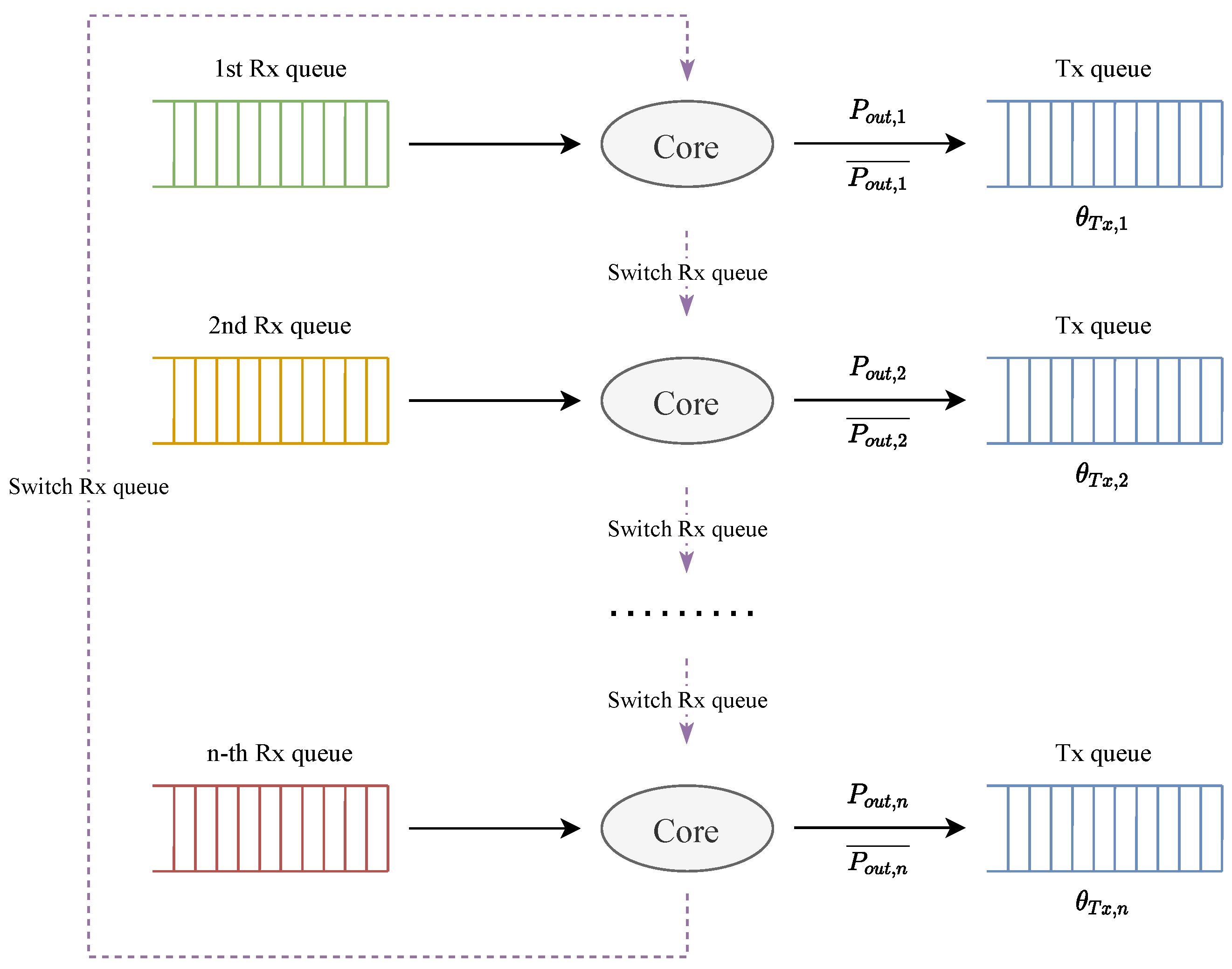
5.2.2. Multiple Rx Queues

Formula (9) is easily extended to multiple Rx queues scenarios. In the case of multiple Rx queues, the packets in each Rx queue may be sent to the same Tx queue. In Section 2.2, we mentioned that, under the spin-polling mechanism, the CPU is polling the Rx queues sequentially, so we can set multiple ${\theta }_{Tx}$ on the Tx queue, corresponding to different Rx queues. This means that when the CPU switches the Rx queue, the ${\theta }_{Tx}$ of the Tx queue need to be changed as well, as shown in Figure 9. When the CPU finishes processing the packets of the i-th Rx queue, $P_{out,i}$ of them are put into the Tx queue. The $\overline{P_{out,i}}$ is the average number of packets from the i-th Rx queue entering the Tx queue per round in $T_{observed}$. Finally, our packet latency optimization strategy in a multiple Rx queues scenario can be represented by the following formula:

$${\theta }_{Tx,i}=\left\{\begin{array}{c}{P}_{out,i},\eta ⩽H\hfill \\ f\left(\overline{P_{out,i}}\right),\eta >H\hfill \end{array}\right.$$

(10)

Figure 9. The multiple Rx queues.

5.3. Two-State Finite State Machine

The CPU utilization threshold is an essential parameter related to when our data plane switches strategies. It is worth noting that if the CPU utilization $\eta$ oscillates around H, our data plane will switch strategies frequently, which inevitably brings unnecessary overhead, so we introduce a two-state finite state machine (FSM) to solve this problem. The two-state FSM we designed is shown in Figure 10. When the data plane runs on $S_0$, it will switch to $S_1$ if $\eta <\alpha H$. When the data plane runs on the $S_1$ state, it will switch to $S_0$ if $\eta >\beta H$. Note that we need to make sure that $0<\alpha <\beta ,\beta H<100\%$, e.g., $\alpha$ = 0.9 and $\beta$ = 1. The use of the FSM can effectively cope with CPU utilization oscillating around a single threshold, thus reducing the frequency of data plane switching strategies.

Figure 10. The two-state finite state machine.

6. Evaluation

Consistent with the test conditions in Section 3.2, we still use the L4 forwarding application built on the ip_pipeline provided by DPDK to evaluate our scheme. In general, the Tx queue length in DPDK is coupled with ${\theta }_{Tx}$. We can make the length of the Tx queue decoupled from ${\theta }_{Tx}$ by a simple code modification, and make ${\theta }_{Tx}$ dynamically adjustable at program runtime. We can do this easily due to the open source nature of DPDK, and this also applies to similar open source high-performance packet processing frameworks. In addition, for comparison, we also implemented Smart Batching [19] on our software data plane. The testbed used in this section is the same as in Section 3.2, as shown in Figure 3a. Specifically, we used a Dell R740 server running our software data plane and an Intel E810 NIC (4 × 25 Gbps mode) to send and receive packets. In addition, an Ixia XGS12 network test platform is our packet generator. Other detailed configuration information is shown in Table 1. Unless otherwise specified, we use 512-byte fixed-length IPv6 TCP packets for experiments, and some flow tables and flow entries are installed on the data plane to support packets forwarding.

6.1. The Selection of Observation Time

Our strategy requires setting two parameters, one is the observation time $T_{observed}$, and the other is the CPU utilization threshold H. The observation time $T_{observed}$ determines how often the data plane calculates CPU utilization and counts the rate at which the Tx queue receives packets. The concern is whether too high a computation frequency will affect the performance of the data plane. We mentioned in the previous section that the most critical performance metric for the data plane is the maximum throughput rate, followed by the latency. Our latency optimization strategy should not adversely affect the maximum throughput rate of the data plane. Therefore, we evaluate the impact of different observation times $T_{observed}$ on the maximum throughput rate of the data plane. To make the results more intuitive, we still use the topology as shown in Figure 3b. We measure the maximum throughput rate of the data plane with our design for observation times $T_{observed}$ equal to 10 s, 1 s, 0.1 s, 0.01 s and 0.001 s, respectively. The experimental results are shown in Figure 11. The standard reference line in Figure 11 is the maximum throughput rate when the data plane is not using our scheme. The experimental results show that the additional overhead incurred by our design using the five observation time parameters described above is insufficient to impact the data plane’s maximum throughput rate significantly. The CPU utilization of the data plane also does not fluctuate drastically in a very short time so that the $T_{observed}$ can be chosen between 0.1 s and 1 s.

Figure 11. The maximum throughput rate of data plane at different observation times.

6.2. The Selection of Threshold

On the other hand, the choice of the threshold H is also quite critical because the choice of the threshold H for CPU utilization determines when the data plane switches strategies. From Figure 5 in Section 3.2, we can see that most of the latency curves start to rise when the input rate exceeds 10 Gbps, so that we can choose the CPU utilization at this point as our threshold H. Moreover, the CPU utilization of the data plane varies at different ${\theta }_{Tx}$. Table 3 shows the CPU utilization of the data plane at an input rate of 10 Gbps for different ${\theta }_{Tx}$. As seen in Table 3, when the input rate is at 10 Gbps, the CPU utilization is around 63%, except for the case ${\theta }_{Tx}=4$. This is because the CPU utilization rises more significantly the closer the input rate is to the maximum throughput rate. In addition, the smaller ${\theta }_{Tx}$ is, the smaller the maximum throughput rate of the data plane is. The starting point of our scheme is to make full use of the CPU to reduce the packet latency, so we should choose as small a threshold as possible. Thus, we can choose the CPU utilization at ${\theta }_{Tx}=64$ as the threshold H of our scheme.

Table 3. The CPU utilization of the data plane at 10 Gbps for different ${\theta }_{Tx}$.

${\mathit{\theta }}_{\mathit{T}\mathit{x}}$	CPU Utilization
4	82.04%
8	64.2%
16	63.11%
32	63.54%
64	63.62%

6.3. Comparison with Other Schemes

In this section, we evaluate the performance of each scheme in the scenario of a single Rx queue. The original data plane, as well as Smart Batching [19], is used to compare with our design. In the original data plane, we set ${\theta }_{Rx}$ to 64 and ${\theta }_{Tx}$ to 64, which is the most general configuration. We use the parameters recommended in their paper for the Smart Batching scheme and set ${\theta }_{Tx}$ to 64. In our scheme, ${\theta }_{Rx}$ is set to 64, $T_{observed}$ to 1 s, and $\eta$ to 60%. The evaluation environment uses the topology of a single Rx queue, shown in Figure 3b. We measured the forwarding latency metrics for each scheme when the total input rate is increased from 1 Gbps to 15 Gbps. Note that according to the maximum throughput rates measured in Section 6.1, the data plane typically does not generate packet loss when the input traffic rate is in the [0, 15] Gbps range, so we do not discuss packet loss rates here. Figure 12a shows the performance of each scheme in terms of average forwarding latency. The forwarding latency of the Smart Batching scheme is almost the same as the original data plane. The Smart Batching scheme optimizes the forwarding latency based on A. However, the mechanism of A has been changed by the current IO frameworks such as DPDK. It is already difficult for the Smart Batching scheme to optimize the forwarding latency by dynamically adjusting A. The difference between the forwarding latency of our scheme and the original data plane and Smart Batching scheme at input rates below 8 Gbps is not significant but still lower than the latter two. In the [0, 8] Gbps interval, our scheme’s maximum reduction in forwarding latency is about 3.56% relative to the original data plane (at an input rate of 5 Gbps). However, starting from 8 Gbps, the advantage of our scheme starts to emerge as the input rate keeps increasing. Compared to the original data plane, the forwarding latency of our scheme is reduced by up to about 45% (at an input rate of 12 Gbps).

Figure 12. The performance of each scheme on single queue scenario. (a) The average latency of each scheme under different input rates. (b) The CPU utilization of each scheme under different input rates.

We also measured the CPU utilization for each scheme, as shown in Figure 12b. Relative to the original data plane, the CPU utilization of our scheme is slightly improved by one or two percentage points. The original data plane suffers from the much-wasted performance at low input rates. Our scheme utilizes a small fraction of the wasted performance to optimize the forwarding latency.

6.4. Multiple Queue Evaluation

The multiple queue scenario is more common than the single queue scenario. Although the multiple queue scenario is complex, and it is not easy to find a representative case for evaluation, we still try to evaluate our scheme using the experimental topology shown in Figure 13. We use Ixia to send 1000 different flows for each NIC port separately, and the data plane hashes the five-tuple of received packets and sends them to the corresponding Tx queues based on the computed hash values. Each network port has the same input rate. We measured the forwarding latency metrics for each scheme when the total input rate is increased from 1 Gbps to 15 Gbps.

Figure 13. The topology of multiple queue evaluation.

Figure 14a shows the performance of each scheme in terms of average forwarding latency. In the [0, 8] Gbps interval, our scheme’s maximum reduction in forwarding latency is about 4.35% relative to the original data plane (at an input rate of 4 Gbps). And in the [9, 15] Gbps interval, the maximum reduction is about 55.54% (at an input rate of 13 Gbps). In terms of the original data plane, there is a significant increase in forwarding latency (up to 32%) for input rates above 9 Gbps relative to the single queue scenario. This is because the average forwarding latency of the software data plane under the spin-polling mechanism rises with the number of queues, which is discussed in detail in paper [6]. Since this is not the focus of this paper, we do not go into depth. The forwarding latency performance of the Smart Batching scheme is also comparable to, or even slightly worse than, that of the original data plane. Figure 14b shows the CPU utilization of each scheme. The CPU utilization of our scheme is slightly more improved, but still not enough to fully utilize the performance of the software data plane at low input rates.

Figure 14. The performance of each scheme on multiple queue scenario. (a) The average latency of each scheme under different input rates. (b) The CPU utilization of each scheme under different input rates.

7. Conclusions and Discussion

The software data plane based on the spin-polling mechanism considerably improves maximum throughput rate and forwarding latency compared with the traditional software data plane. However, there is still a performance waste problem. Meanwhile, the batch processing mechanism of the software data plane does not cope well with different input traffic rates. We propose a dynamic adjustment method for output batch size, which aims to utilize the wasted CPU core cycles to optimize the forwarding latency of the software data plane. Experimental results show that in a single-queue scenario, compared with the original data plane, our scheme can reduce the forwarding latency by up to 45% and this optimization effect can reach up to 55.54% in an evaluation for the multiple queue scenario.

The CPU cores of the software data plane based on the spin-polling are always running full-tilt, but the CPU utilization is not high at all times. Our work optimizes the forwarding latency by dynamically adjusting the output batch size, which improves the CPU utilization. Nevertheless, the CPU utilization is still low at low input traffic rates, which means that data plane may have some room for performance improvement. Making full use of CPU to improve the performance of data plane and solving the problem of energy consumption are two aspects of our future work.

References

1. DPDK: Data Plane Development Kit. Available online: https://www.dpdk.org/ (accessed on 25 July 2022).
2. Wang, J.; Cheng, G.; You, J.; Sun, P. SEANet: Architecture and Technologies of an On-Site, Elastic, Autonomous Network. J. Netw. New Media 2020, 6, 1–8. [Google Scholar]
3. Rawat, D.B.; Reddy, S.R. Software Defined Networking Architecture, Security and Energy Efficiency: A Survey. IEEE Commun. Surv. Tutor. 2017, 19, 325–346. [Google Scholar] [CrossRef]
4. Masoudi, R.; Ghaffari, A. Software Defined Networks: A Survey. J. Netw. Comput. Appl. 2016, 67, 1–25. [Google Scholar] [CrossRef]
5. Open vSwitch. Available online: http://www.openvswitch.org/ (accessed on 25 July 2022).
6. Golestani, H.; Mirhosseini, A.; Wenisch, T.F. Software Data Planes: You Can’t Always Spin to Win. In Proceedings of the ACM Symposium on Cloud Computing, Santa Cruz, CA, USA, 20–23 November 2019; ACM: New York, NY, USA, 2019; pp. 337–350. [Google Scholar] [CrossRef]
7. Lim, H.; Han, D.; Andersen, D.G.; Kaminsky, M. MICA: A Holistic Approach to Fast In-Memory Key-Value Storage. In Proceedings of the 11th USENIX Symposium on Networked Systems Design and Implementation, Seattle, WA, USA, 2–4 April 2014; p. 17. [Google Scholar]
8. Marinos, I.; Watson, R.N.; Handley, M. Network Stack Specialization for Performance. In Proceedings of the 2014 ACM Conference on SIGCOMM, Chicago, IL, USA, 17–22 August 2014; pp. 175–186. [Google Scholar] [CrossRef]
9. Jeong, E.; Woo, S.; Jamshed, M.; Jeong, H.; Ihm, S.; Han, D.; Park, K. mTCP: A Highly Scalable User-Level TCP Stack for Multicore Systems. In Proceedings of the 11th USENIX Symposium on Networked Systems Design and Implementation, Seattle, WA, USA, 2–4 April 2014; p. 15. [Google Scholar]
10. Kalia, A.; Andersen, D. Datacenter RPCs Can Be General and Fast. In Proceedings of the 16th USENIX Symposium on Networked Systems Design and Implementation, Boston, MA, USA, 26–28 February 2019; p. 17. [Google Scholar]
11. Peter, S.; Li, J.; Zhang, I.; Ports, D.R.K.; Woos, D.; Krishnamurthy, A.; Anderson, T.; Roscoe, T. Arrakis: The Operating System Is the Control Plane. ACM Trans. Comput. Syst. 2016, 33, 1–30. [Google Scholar] [CrossRef]
12. Belay, A.; Prekas, G.; Kozyrakis, C.; Klimovic, A.; Grossman, S.; Bugnion, E. IX: A Protected Dataplane Operating System for High Throughput and Low Latency. In Proceedings of the 11th USENIX Symposium on Operating Systems Design and Implementation, Broomfield, CO, USA, 6–8 October 2014; p. 18. [Google Scholar]
13. Prekas, G.; Kogias, M.; Bugnion, E. ZygOS: Achieving Low Tail Latency for Microsecond-scale Networked Tasks. In Proceedings of the 26th Symposium on Operating Systems Principles, Shanghai, China, 28–31 October 2017; pp. 325–341. [Google Scholar] [CrossRef]
14. Ousterhout, A.; Fried, J.; Behrens, J.; Belay, A.; Balakrishnan, H. Shenango: Achieving High CPU Efficiency for Latency-sensitive Datacenter Workloads. In Proceedings of the 16th USENIX Conference on Networked Systems Design and Implementation, Boston, MA, USA, 26–28 February 2019; p. 18. [Google Scholar]
15. Kaffes, K.; Belay, A.; Chong, T.; Mazieres, D.; Humphries, J.T.; Kozyrakis, C. Shinjuku: Preemptive Scheduling for Msecond-Scale Tail Latency. In Proceedings of the 16th USENIX Conference on Networked Systems Design and Implementation, Boston, MA, USA, 26–28 February 2019; p. 16. [Google Scholar]
16. Dalton, M.; Schultz, D.; Adriaens, J.; Arefin, A.; Gupta, A.; Fahs, B.; Rubinstein, D.; Zermeno, E.C.; Rubow, E.; Docauer, J.A.; et al. Andromeda: Performance, Isolation, and Velocity at Scale in Cloud Network Virtualization. In Proceedings of the 15th USENIX Symposium on Networked Systems Design and Implementation, Renton, WA, USA, 9–11 April 2018; p. 16. [Google Scholar]
17. Honda, M.; Lettieri, G.; Eggert, L.; Santry, D. PASTE: A Network Programming Interface for Non-Volatile Main Memory. In Proceedings of the 15th USENIX Symposium on Networked Systems Design and Implementation, Renton, WA, USA, 9–11 April 2018; p. 18. [Google Scholar]
18. Klimovic, A.; Litz, H.; Kozyrakis, C. ReFlex: Remote Flash ≈ Local Flash. In Proceedings of the Twenty-Second International Conference on Architectural Supportfor Programming Languages and Operating Systems, Xi’an, China, 8–12 April 2017; pp. 345–359. [Google Scholar] [CrossRef]
19. Miao, M.; Cheng, W.; Ren, F.; Xie, J. Smart Batching: A Load-Sensitive Self-Tuning Packet I/O Using Dynamic Batch Sizing. In Proceedings of the 2016 IEEE 18th International Conference on High Performance Computing and Communications, IEEE 14th International Conference on Smart City, IEEE 2nd International Conference on Data Science and Systems (HPCC/SmartCity/DSS), Sydney, Australia, 16 December 2016; pp. 726–733. [Google Scholar] [CrossRef]
20. Lange, S.; Linguaglossa, L.; Geissler, S.; Rossi, D.; Zinner, T. Discrete-Time Modeling of NFV Accelerators That Exploit Batched Processing. In Proceedings of the IEEE INFOCOM 2019-IEEE Conference on Computer Communications, Paris, France, 29 April–2 May 2019; pp. 64–72. [Google Scholar] [CrossRef]
21. Das, T.; Zhong, Y.; Stoica, I.; Shenker, S. Adaptive Stream Processing Using Dynamic Batch Sizing. In Proceedings of the ACM Symposium on Cloud Computing—SOCC ’14, Seattle, WA, USA, 3–5 November 2014; pp. 1–13. [Google Scholar] [CrossRef] [Green Version]
22. Cerovic, D.; Del Piccolo, V.; Amamou, A.; Haddadou, K.; Pujolle, G. Fast Packet Processing: A Survey. IEEE Commun. Surv. Tutor. 2018, 20, 3645–3676. [Google Scholar] [CrossRef]
23. Kim, J.; Huh, S.; Jang, K.; Park, K.; Moon, S. The Power of Batching in the Click Modular Router. In Proceedings of the APSYS ’12: Proceedings of the Asia-Pacific Workshop on Systems, Seoul, Korea, 23–24 July 2012; p. 6. [Google Scholar]
24. Barroso, L.A.; Hölzle, U. The Case for Energy-Proportional Computing. Computer 2007, 40, 33–37. [Google Scholar] [CrossRef]
25. McKeown, N.; Anderson, T.; Balakrishnan, H.; Parulkar, G.; Peterson, L.; Rexford, J.; Shenker, S.; Turner, J. OpenFlow: Enabling Innovation in Campus Networks. SIGCOMM Comput. Commun. Rev. 2008, 38, 69–74. [Google Scholar] [CrossRef]
26. Li, S.; Hu, D.; Fang, W.; Ma, S.; Chen, C.; Huang, H.; Zhu, Z. Protocol Oblivious Forwarding (POF): Software-Defined Networking with Enhanced Programmability. IEEE Netw. 2017, 31, 9. [Google Scholar] [CrossRef]
27. Bosshart, P.; Daly, D.; Gibb, G.; Izzard, M.; McKeown, N.; Rexford, J.; Schlesinger, C.; Talayco, D.; Vahdat, A.; Varghese, G.; et al. P4: Programming Protocol-Independent Packet Processors. ACM SIGCOMM Comput. Commun. Rev. 2014, 44, 87–95. [Google Scholar] [CrossRef]
28. Kim, H.J.; Lee, Y.S.; Kim, J.S. NVMeDirect: A User-Space I/O Framework for Application-specific Optimization on NVMe SSDs. In Proceedings of the 8th USENIX Conference on Hot Topics in Storage and File Systems, Denver, CO, USA, 20–21 June 2016; p. 5. [Google Scholar]
29. Yang, Z.; Liu, C.; Zhou, Y.; Liu, X.; Cao, G. SPDK Vhost-NVMe: Accelerating I/Os in Virtual Machines on NVMe SSDs via User Space Vhost Target. In Proceedings of the 2018 IEEE 8th International Symposium on Cloud and Service Computing (SC2), Paris, France, 18–21 November 2018; pp. 67–76. [Google Scholar] [CrossRef]
30. Begin, T.; Baynat, B.; Artero Gallardo, G.; Jardin, V. An Accurate and Efficient Modeling Framework for the Performance Evaluation of DPDK-Based Virtual Switches. IEEE Trans. Netw. Serv. Manag. 2018, 15, 1407–1421. [Google Scholar] [CrossRef]
31. Han, S.; Jang, K.; Park, K.; Moon, S. PacketShader: A GPU-Accelerated Software Router. In ACM SIGCOMM Computer Communication Review; ACM: New York, NY, USA, 2010; p. 12. [Google Scholar]
32. Rizzo, L. Netmap: A Novel Framework for Fast Packet I/O. In Proceedings of the USENIX ATC ’12: USENIX Annual Technical Conference, Boston, MA, USA, 12–15 June 2012; USENIX Association: Berkeley, CA, USA, 2012; p. 12. [Google Scholar]
33. PF_RING. 2011. Available online: https://www.ntop.org/products/packet-capture/pf_ring/ (accessed on 25 July 2022).
34. OpenOnload. 2022. Available online: https://github.com/Xilinx-CNS/onload (accessed on 25 July 2022).
35. PACKET_MMAP. Available online: https://www.kernel.org/doc/Documentation/networking/packet_mmap.txt (accessed on 25 July 2022).
Publisher’s Note: MDPI stays neutral with regard to jurisdictional claims in published maps and institutional affiliations.
Article Metrics
Citations
Article Access Statistics
Multiple requests from the same IP address are counted as one view.