Study of an Atmospheric Refractivity Estimation from a Clutter Using Genetic Algorithm

Featured Application

This article is related to atmospheric refractivity estimation from clutter images using a genetic algorithm.

Abstract

In this paper, a method for estimating atmospheric refractivity from sea and land clutters is proposed. To estimate the atmospheric refractivity, clutter power spectrums based on an artificial tri-linear model are calculated using an Advanced Refractive Prediction System (AREPS) simulator. Then, the clutter power spectrums are again obtained based on the measured atmospheric refractivity data using the AREPS simulator. In actual operation, this spectrum from measured reflectivity can be replaced with real-time clutter spectrums collected from radars. A cost function for the genetic algorithm (GA) is then defined based on the difference between the two clutter power spectrums to predict the atmospheric refractivity using the artificial tri-linear model. The optimum variables of the tri-linear model are determined at a minimum cost in the GA process. The results demonstrate that atmospheric refractivity can be predicted using the proposed method from the clutter powers.

1. Introduction

Advancements in radar technologies have led to significant improvements in the performance of long-range shipborne radar systems, which have been extensively adopted for searching and tracking enemy targets [1,2,3,4,5]. However, in such radar systems, the radar performance is sometimes degraded by weather conditions [6,7,8,9], because the propagation path of the radar signal varies when the atmospheric refractivity changes. Therefore, long-range shipborne radar systems require a real-time observation of the atmospheric conditions. To observe atmospheric conditions, a rawinsonde that can measure the atmospheric conditions at high altitude is typically used [10,11,12]. However, it is difficult to obtain the atmospheric conditions in real-time since the rawinsonde is generally operated for a limited time of less than three times a day. To achieve real-time observations of atmospheric conditions, several studies focusing on estimating refractivity from clutter (RFC) have been conducted. The RFC techniques utilizing radar sea-clutter images are often combined with various estimation methods, such as the Kalman filter [13], Monte Carlo simulation [14], and other optimization algorithms [15,16,17,18]. However, most of these studies have been conducted within the limited space around Wallops Island [13,14,15,16,17,18,19]. In addition, since the radar sea-clutter images are significantly affected by the sea wave height, it is difficult to obtain constant images, even if the atmospheric environment is assumed to be the same [20,21,22]. More recently, a study on sea-surface modeling using a deep learning method that recognizes the real-time changing state of sea waves has been reported [23].

In this paper, a method for estimating the atmospheric refractivity using both the sea and land clutters is proposed. The atmospheric refractivity can be estimated using the clutter powers, because the clutter powers are varied in real-time depending on the atmospheric refractivity. Since land clutter powers do not change much if the atmospheric environment is constant [24], the clutter powers should be obtained not only for the sea but also for the land. In the actual radar operation, more consistent prediction results can be obtained by analyzing clutter, including land terrain. To estimate the atmospheric refractivity using the clutter powers, the real terrain model around a coastal area, including a number of islands and inland in Korea, is applied to Advanced Refractive Prediction System (AREPS) electromagnetic (EM) propagation simulation software [25]. Then, different RCS models are applied to land and sea. In addition, an artificial tri-linear model that can express all atmospheric conditions, including normal, super, sub and duct, is designed. Based on the artificial tri-linear model, the clutter power spectrums are calculated using the AREPS EM simulator. At the same time, the clutter power spectrums are again obtained based on the measured atmospheric refractivity data using the AREPS simulator. Herein, data from four dates, including the duct condition among the 2021 data measured by the Heuksando Meteorological Observatory, are utilized. In actual operation, this spectrum of measured reflectivity can be replaced with real-time clutter spectrums collected from radars. A cost function for the genetic algorithm (GA) is then defined based on the difference between the use of the two calculated clutter power spectrums to predict the atmospheric refractivity. The optimum variables of the tri-linear model are determined at a minimum cost in the GA process. The results demonstrate that atmospheric refractivity can be predicted from the clutter powers using the proposed method.

2. Calculation of Clutter Power Spectrums

Figure 1 presents the propagation of the electromagnetic wave of the shipborne radar systems according to atmospheric conditions, including normal, sub, super, and duct. The atmospheric conditions are classified by the gradient of modified refractive index M in terms of the altitudes. The modified refractive index M can be calculated using the following equation [26]:

$$N=\left(77.6\times {10}^{-6}\times \frac{P}{T}+0.373\times \frac{e}{T^2}\right)\times {10}^6$$

(1)

$$M=N+0.157\times h$$

(2)

where N is the refractive index, P is the air pressure in millibars, e is the water vapor pressure in millibars, and T is the absolute temperature in K. The refractivity of N is replaced by the modified refractivity of M to take into consideration the Earth’s curvature according to altitude h. Normal refraction occurs when the gradient of the refractivity is 78 ≤ ∇M ≤ 157, which indicates good conditions for radar systems to search for a target. However, when the ∇M is greater (sub, ∇M > 157) or less (super, 0 < ∇M < 78) than the normal state, shipborne radar systems find it difficult to observe the exact distance and altitude of the targets due to abnormal refraction of the radio waves. Moreover, in the duct condition (∇M < 0), the wave propagation of the radar signal is trapped as if in a waveguide. Therefore, it is important to be able to anticipate atmospheric refractivity to prevent degradation of radar performance depending on the atmospheric conditions.

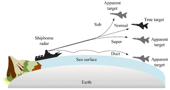
Figure 1. Wave propagation of the shipborne radar according to atmospheric conditions.

Figure 2 shows the observation area and scan range for obtaining the clutter power spectrum. In our analysis, the shipborne radar is located near Wando, which illuminates the north direction with a scan range of 20° (φ = 80°~100°) to obtain the clutter power spectrums from both the land and sea. Herein, the sea clutter powers are significantly affected by the sea wave height, whereas the land clutter powers do not change substantially as long as the atmospheric environment remains constant. Thus, when the radar obtains the clutter powers by illuminating not only the sea but also the land, atmospheric refractivity can be predicted more accurately.

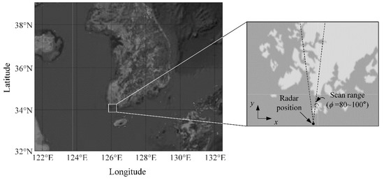
Figure 2. Observation area and scan range of the shipborne radar systems.

Figure 3 presents the measured atmospheric refractivity data when atmospheric conditions are duct or normal. These data were measured at different times in the Heuksando Meteorological Observatory [27], which is the closest meteorological station to Wando. In this measurement data, Case 5 is the normal condition, whereas Cases 1, 2, 3, and 4 represent duct conditions with duct slopes (∇M) of −121, −159, −121, and −151, respectively.

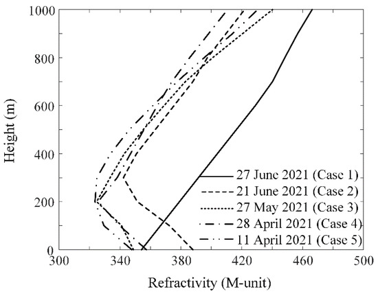
Figure 3. Comparison of the measured atmospheric refractivity for the different atmospheric conditions.

Figure 4 illustrates the propagation factor according to different atmospheric conditions with the measurement data of Case 1 (normal) and Case 2 (duct). The solid black lines indicate the height of the terrain around Wando, and the terrain data are obtained from the NASA earth data center [28]. In this simulation, the radar height is assumed to be 30 m, and the observation range and altitude are 0 to 100 km and 0 to 1000 m, respectively. When the atmospheric condition is normal, radar wave propagation is disturbed by the high topography, so the shaded areas are clearly observed, as shown in Figure 4a. In contrast, when ducting occurs, a strong propagation factor is observed even behind the high terrain. The result means that the radar can have completely different propagation paths depending on the atmospheric conditions.

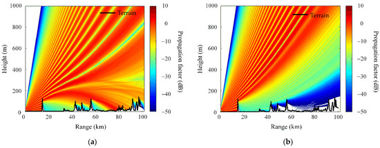
Figure 4. Propagation factor according to different atmospheric conditions in the duct and normal: (a) using the measured data of Case 1; (b) using the measured data of Case 2.

Figure 5 shows the clutter power spectrum according to the atmospheric conditions. The clutter power can be calculated from the propagation factor using the following equations [29]:

$$A=\frac{r\theta c\tau }{2}$$

(3)

$$P_c=\frac{P_t{G}^2{\lambda }^{2}A{\sigma }_0}{{(4\pi )}^3{r}^4}$$

(4)

where P_t is the transmitted power, and G is the antenna gain of the radar, λ is the wavelength, and r is the range of the radar for the observation location. In addition, A is the illumination surface area by the radar signal, which can be obtained from range r, antenna beamwidth θ, light speed c, and radar pulse width τ. σ₀ refers to the radar cross section (RCS) of the land [24] and sea surface [20]. Generally, the RCS for the land surface is higher than for the sea surface. When the atmospheric condition is normal, the strong clutter power spectrum is not observed over a range of 20 km, as shown in Figure 5a, because the high terrain blocks the wave propagation. On the other hand, when the atmospheric condition is duct, a strong clutter power is observed in a wide range, as shown in Figure 5b.

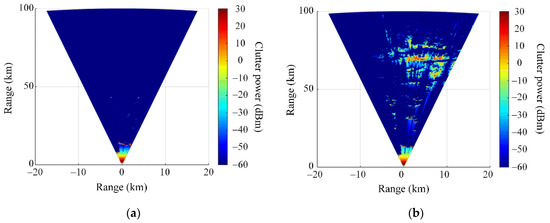
Figure 5. Clutter power spectrums according to atmospheric conditions: (a) using the measured data of Case 1; (b) using the measured data of Case 2.

3. Estimation of an Atmospheric Refractivity

Figure 6 shows the shape of the tri-linear model for the atmospheric refractivity estimation method. The artificial tri-linear model consists of three lines with slopes d₁, d₂, and d₃. In addition, the boundaries between the three lines are determined by h₁ and h₂. Since the slope of the tri-linear model can be changed to negative or positive values, the tri-linear model can express most atmospheric conditions, including normal, super, sub, and duct. Therefore, the tri-linear model can be utilized as an approximate atmospheric refractivity model in refractivity estimation methods.

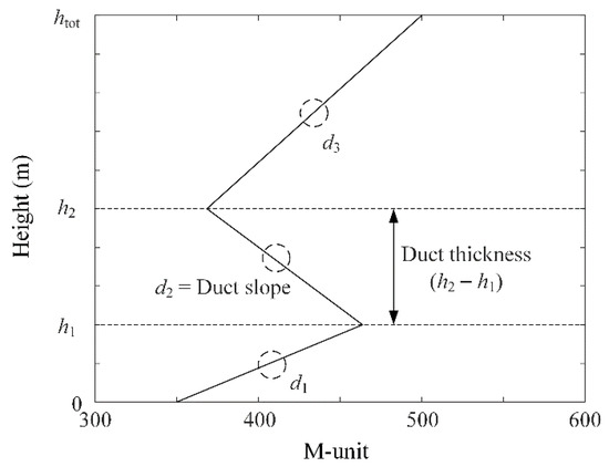
Figure 6. The shape of the tri-linear model.

Figure 7 presents the flow chart of the use of the GA algorithm [17,18] to predict the atmospheric refractivity from the clutter power spectrums. To predict the atmospheric refractivity, a random chromosome is first generated, and then the decoded values from the chromosome are applied to the variables of the tri-linear model. The tri-linear model is used as input to the AREPS EM propagation simulator to calculate the clutter power spectrum. At the same time, the clutter power spectrums are again obtained based on the measured atmospheric refractivity data introduced in Figure 3 using the AREPS simulator. In actual operation, this spectrum of measured reflectivity can be replaced with real-time clutter spectrums collected from radars. Herein, the cost function for the GA is then defined based on the difference between the two calculated clutter power spectrums. In the GA process, the variables of the tri-linear model are adjusted to minimize the cost through the reproduction process. Consequently, the optimum variables of the tri-linear model are determined at a minimum cost in the GA, which means that the estimated atmospheric conditions have been obtained. The GA parameters, such as population size, generations, and mutation ratio, are listed in Table 1.

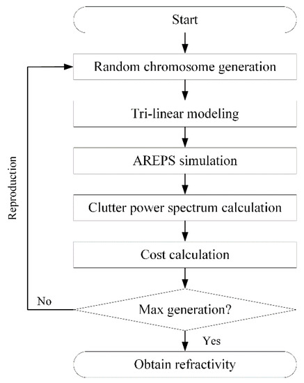
Figure 7. GA process for estimating atmospheric refractivity.

Table 1. Detailed information of the GA.

Option	Value
Population size	30
Generations	15
Elite count	6
Crossover ratio	40%
Mutation ratio	10%

Figure 8 provides a comparison of the estimated and measured atmospheric refractivity data based on the clutter powers. Estimation is conducted for the measured data in Figure 3, and the duct slopes and duct thickness of the estimated and measured values are summarized in Table 2. Based on the results shown in Table 2, the estimation errors for the duct slopes and duct thickness are maintained at below 46.1 and 36, respectively. For Case 3, the atmospheric refractivity can estimate with estimation errors for the duct slopes and duct thickness of 29 and 24, respectively. This estimation result of the best case is compared with other studies in Table 3. The results demonstrate that the atmospheric refractivity can be predicted from clutter powers using the proposed method. The proposed method is suitable for actual radar systems because it is possible to obtain more consistent prediction results by analyzing clutter, including land terrain, when operating the actual radar.

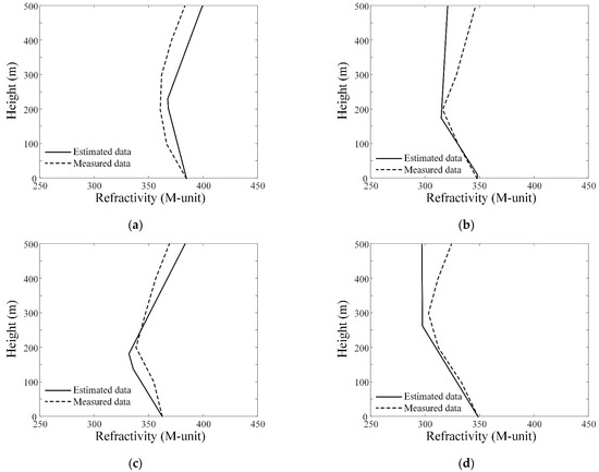
Figure 8. Comparison of the estimated and real atmospheric refractivity. (a) Using the measured data of Case 2; (b) using the measured data of Case 3; (c) using the measured data of Case 4; (d) using the measured data of Case 5.

Table 2. Summary of all estimation results.

Case	Duct Slopes (Esti.)	Duct Slopes (Mea.)	Duct Thickness (Esti.)	Duct Thickness (Mea.)
Case 2	−74.9	−121	231	200
Case 3	−187.5	−158.5	176	200
Case 4	−168.7	−121	181.5	200
Case 5	−194.3	−151	264	300

Table 3. Comparison results.

Option	[14]	[17]	Our Best
Duct slopes error	4	240	29
Duct thickness error	0.14	47	24

4. Conclusions

In this paper, we have investigated the method for estimating atmospheric refractivity using both sea and land clutters. To estimate the atmospheric refractivity, the artificial tri-linear model that can express all atmospheric conditions was applied in a GA process. In addition, the clutter power spectrum was calculated using an AREPS EM propagation simulator. At the same time, the clutter power spectrums were again obtained based on the measured atmospheric refractivity data. The cost function for the GA was then defined based on the difference between the two clutter power spectrums. From the estimation result, the estimation errors for the duct slopes and duct thickness were maintained at below 46.1 and 36, respectively. The results demonstrated that atmospheric refractivity can be predicted using the proposed method from the clutter powers.

References

- Locker, C.; Vaupel, T.; Eibert, T.F. Radiation efficient unidirectional low-profile slot antenna elements for X-band application. IEEE Trans. Antennas Propag. 2005, 53, 2765–2768. [Google Scholar] [CrossRef]
- Dastkhosh, A.R.; Oskouei, H.D.; Khademevatan, G. Compact low weight high gain broadband antenna by polarization-rotation technique for X-band radar. Int. J. Antennas Propag. 2014, 2014, 743046. [Google Scholar] [CrossRef]
- Zhou, Y.; Wang, T.; Hu, R.; Su, H.; Liu, Y.; Liu, X.; Suo, J.; Snoussi, H. Multiple kernelized correlation filters (MKCF) for extended object tracking using X-band marine radar data. IEEE Trans. Signal Process. 2019, 67, 3676–3688. [Google Scholar] [CrossRef]
- Wang, A.; Krishnamurthy, V. Signal interpretation of multifunction radars: Modeling and statistical signal processing with Stochastic Context Free Grammar. IEEE Trans. Signal Process. 2008, 56, 1106–1119. [Google Scholar] [CrossRef]
- Wang, S.; Jang, D.; Kim, Y.; Choo, H. Design of S/X-Band dual-loop shared-aperture 2 × 2 array antenna. J. Electromagn. Eng. Sci. 2022, 22, 319–325. [Google Scholar] [CrossRef]
- Lim, T.H.; Go, M.; Seo, C.; Choo, H. Analysis of the target detection performance of Air-to-Air airborne radar using long-range propagation simulation in abnormal atmospheric conditions. Appl. Sci. 2020, 10, 6440. [Google Scholar] [CrossRef]
- Lim, T.; Choo, H. Prediction of target detection probability based on air-to-air long-range scenarios in anomalous atmospheric environments. Remote Sens. 2021, 13, 3943. [Google Scholar] [CrossRef]
- Sharma, V.; Kumar, L. Photonic-radar based multiple-target tracking under complex traffic-environments. IEEE Access 2020, 8, 225845–225856. [Google Scholar] [CrossRef]
- Kim, I.; Kim, H.; Lee, J.-H. Theoretical minimum detection range for a rapidly moving target and an experimental evaluation. J. Electromagn. Eng. Sci. 2021, 21, 161–164. [Google Scholar] [CrossRef]
- Tedesco, M.; Wang, J.R. Atmospheric correction of AMSR-E brightness temperatures for dry snow cover mapping. IEEE Geosci. Remote Sens. Lett. 2006, 3, 320–324. [Google Scholar] [CrossRef]
- Wang, J.R.; Racette, P.; Triesky, M.E.; Browell, E.V.; Ismail, S.; Chang, L.A. Profiling of atmospheric water vapor with MIR and LASE. IEEE Geosci. Remote Sens. Lett. 2002, 40, 1211–1219. [Google Scholar] [CrossRef]
- Birkemeier, W.P.; Duvosin, P.F.; Fontaine, A.B.; Thomson, D.W. Indirect atmospheric measurements utilizing rake tropospheric scatter techniques—Part II: Radiometeorological interpretation of rake channel-sounding observations. Proc. IEEE 1969, 57, 552–559. [Google Scholar] [CrossRef]
- Yardim, C.; Gerstoft, P.; Hodgkiss, W.S. Tracking refractivity from clutter using Kalman and Particle filters. IEEE Trans. Antennas Propag. 2008, 56, 1058–1070. [Google Scholar] [CrossRef]
- Yardim, C.; Gerstoft, P.; Hodgkiss, W.S. Estimation of radio refractivity from radar clutter using Bayesian Monte Carlo analysis. IEEE Trans. Antennas Propag. 2006, 54, 1318–1327. [Google Scholar] [CrossRef]
- Gerstoft, P.; Rogers, L.T.; Krolik, J.L.; Hodgkiss, W.S. Inversion for refractivity parameters from radar sea clutter. Radio Sci. 2003, 38, 8053. [Google Scholar] [CrossRef]
- Huang, S.-X.; Zhao, X.-F.; Sheng, Z. Refractivity estimation from radar sea clutter. Chin. Phys. B 2009, 18, 5084–5090. [Google Scholar]
- Cemil, T.; Isa, N. A novel hybrid model for inversion problem of atmospheric refractivity estimation. AEU Int. J. Electron. Commun. 2018, 84, 258–264. [Google Scholar]
- Penton, S.E.; Hackett, E.E. Rough ocean surface effects on evaporative duct atmospheric refractivity inversions using genetic algorithms. Radio Sci. 2018, 53, 804–819. [Google Scholar] [CrossRef]
- Karimian, A.; Yardim, C.; Gerstoft, P.; Hodgkiss, W.S.; Barrios, A.E. Refractivity estimation from sea clutter: An invited review. Radio Sci. 2011, 46, RS6013. [Google Scholar] [CrossRef]
- Nathanson, F.E.; Reilly, J.P.; Cohen, M. Radar Design Principles, 2nd ed.; McGraw-Hill: New York, NY, USA, 1991. [Google Scholar]
- Reilly, J.P.; Dockery, G.D. Influence of evaporation ducts on radar sea returns. IEEE Proc. 1990, 137, 80–88. [Google Scholar]
- Vilhelm, G.H.; Rashmi, M. An improved empirical model for radar sea clutter reflectivity. IEEE Trans. Aerosp. Electron. Syst. 2012, 49, 3512–3524. [Google Scholar]
- Ma, L.; Wu, J.; Zhang, J.; Wu, Z.; Jeon, G.; Zhang, Y.; Wu, T. Research on sea clutter reflectivity using deep learning model in industry 4.0. IEEE Trans. Ind. Inform. 2020, 16, 5929–5937. [Google Scholar] [CrossRef]
- Feng, S.; Chen, J. Low-angle reflectivity modeling of land clutter. IEEE Geosci. Remote Sens. Lett. 2006, 3, 254–258. [Google Scholar] [CrossRef]
- Advanced Refractive Prediction System (AREPS); version 3.6; The Space and Naval Warfare System: San Diego, CA, USA, 2005.
- ITU. The Radio Refractive Index: Its Formula and Refractivity Data. ITU-R P.453. 2019. Available online: https://www.itu.int/rec/R-REC-P.453/en (accessed on 8 September 2019).
- University of Wyoming, Department of Atmospheric Science. Available online: https://weather.uwyo.edu/upperair/sounding.html (accessed on 31 January 2022).
- NASA. NASA Earth Data Center. Available online: https://www.earthdata.nasa.gov/ (accessed on 1 January 2022).
- Compaleo, J.; Yardim, C.; Xu, L. Refractivity-from-clutter capable, software-defined, coherent-on-receive marine radar. Radio Sci. 2021, 56, 1–19. [Google Scholar] [CrossRef]
Publisher’s Note: MDPI stays neutral with regard to jurisdictional claims in published maps and institutional affiliations. |
© 2022 by the authors. Licensee MDPI, Basel, Switzerland. This article is an open access article distributed under the terms and conditions of the Creative Commons Attribution (CC BY) license (https://creativecommons.org/licenses/by/4.0/).