The Sky-Status Climatology of Greece: Emphasis on Sunshine Duration and Atmospheric Scattering

Featured Application

The present work examines the distribution of the three types of sky conditions (clear, intermediate, and overcast) over Greece by applying the diffuse-fraction methodology developed by the same author and two other co-workers.

Abstract

The aim of this work is the study of the sky conditions climatology over Greece based on the diffuse-fraction (k_d) limits, for clear, k_d ∈ [0, 0.26]; intermediate, k_d ∈ (0.26, 0.78); and overcast, k_d ∈ (0.78, 1) skies. k_d is, therefore, used here to characterise the sky conditions over a site. Its values are estimated from diffuse and global horizontal solar irradiances the typical meteorological years of 43 selected Greek sites. The k_d values in each specific range are equivalent to sunshine durations (SSDs) under the particular sky conditions. Annual, seasonal, and intra-annual variations in SSDs are estimated with regression equations to fit their means. Clear skies comprise 33%, intermediate 40%, and overcast 27% of the time in a year. k_d, as an atmospheric scattering index (ASI), shows dependence on the sites’ geographical latitude: best-fit lines mean ASIs are derived showing no trend, while overcast skies show a slight negative trend. A comparison of the clear-sky SSDs for four Greek sites from the Global Climate Data and one site from the Academy of Sciences of Moldova with those derived from k_d shows a remarkable difference. A new methodology is developed that results in much smaller differences. Finally, maps of the annual SSDs and ASIs are derived for Greece.

1. Introduction

The notion of sunshine duration (SSD) or bright sunshine hours have been introduced by the World Meteorological Organisation (WMO) in order to indicate the time duration at a site with visible Sun. The SSD parameter is recorded as long as the direct-normal solar irradiance exceeds the value of 120 W⋅m⁻². The sunshine duration is a parameter of secondary significance in the determination of the climatology at a site, while its prime parameters are temperature, humidity, wind, precipitation, and solar radiation. Nevertheless, sunshine duration nowadays plays a significant role in estimating the solar radiation intensity at a location via modelling [1,2].

In addition to the above, sunlight has many other applications. Wei et al. [3] have developed a digital tool for predicting the necessary sunshine for plants. Sanchez-Romero et al. [4] have provided a methodology for reconstructing aerosol-optical-depth (AOD) series from sunshine records. Kothe et al. [5] have derived a satellite-based SSD climate data record for Europe. Katsoulis and Kambezidis [6] and Founda et al. [7] have reported the variations in cloudiness/sunshine and sunshine over Greece, respectively. Van den Bessalar et al. [8] have studied the relationship between SSD and air-temperature trends across Europe, while Bartoszek et al. [9] have investigated the relationships between cloudiness, AOD, and SSD over Poland.

Solar radiation on a horizontal plane (H_g) is the sum of the diffuse (scattered) radiation (H_d) coming from all parts of the sky vault at a site and the direct one (H_b) coming from the Sun exclusively. As H_b can be estimated accurately, it is the other solar component (i.e., H_d) that needs attention, because its estimation is not straightforward due to multiple scattering of the incoming solar radiation in the Earth’s atmosphere by atmospheric molecules, atmospheric aerosols, and clouds. To overcome the difficulty in estimating H_d, many researchers have used the notion of the clearness index (k_t) or of the diffuse fraction (k_d). The first is defined as the ratio of H_g to the extraterrestrial solar radiation (H₀), while k_d is defined as the ratio of H_d to H_g. Use of the k_d has been made in several works [10,11,12,13]. Nevertheless, almost all of them relate k_d as a function of k_t [14,15,16,17].

Engerer [18] has given results from a relevant study about high-temporal resolution estimates of k_d for south-eastern Australia. A similar study for India has been performed by [19]. Salhi et al. [12] evaluated the diffuse fraction and diffuse coefficient from statistical analysis over two sites in Algeria. An interesting work [20] has presented a new methodology to derive typical meteorological years (TMYs) from hourly diffuse-fraction values. Boland et al. [21] have developed a model to estimate the diffuse fraction of solar radiation on a horizontal surface. Nevertheless, none of the above studies or others from the international literature not mentioned here have used k_d to characterise the sky conditions over a site.

Kambezidis et al. [22] have developed a methodology with which the sky is categorised as clear, intermediate, or overcast by only determining the upper and lower limits of the diffuse fraction (k_du and k_dl, respectively). Their methodology has been applied to 14 sites around the world and verified. The authors concluded that the k_du and the k_dl boundaries may take the universal values of 0.78 and 0.26, respectively. Moreover, Kambezidis [23] has used the notion of the diffuse fraction in defining the solar radiation climatology of Greece and has shown that k_d can also be used as an atmospheric scattering parameter.

The present study aims at using k_d to determine the sky conditions in their distribution over Greece according to the methodology developed by [22]. This is the first time worldwide that the mentioned methodology is applied to define the sky status (clear, intermediate, overcast) over a country (Greece in this case) and how these three types of cloudiness are distributed over the area.

The structure of the paper is as follows. Section 2 provides details for the sites used in this work and their corresponding meteorological data within Greece for analysis. Section 3 presents the results of the analysis (annual, seasonal, and monthly variation in k_d over Greece with subsequent maps). Section 4 discusses the weaknesses of the methodology utilised in the present study, as well as the development and use of a new formulation for calculating the sunshine hours, while Section 5 provides the main achievements of the study and gives its conclusions.

2. Materials and Methods

2.1. Data Collection

The data bases of this work are exactly those utilised in the study by Kambezidis [23]. These bases correspond to 43 sites in Greece as selected by Kambezidis [23]; the sites are located in the map of Figure 1. The data bases constitute TMYs for the chosen sites. A TMY is a set of meteorological and solar radiation parameters with hourly values usually; these values cover a whole year for a given location [24]. Moreover, a TMY consists of a set of (typical meteorological) months, which are selected from individual years within a given period by applying the statistical methodology of Filkenstein–Schafer [25]; then, these months are integrated into a complete year [24]. This way, a TMY reflects all the specific climatic information of the location for the period it has been generated from. The advantage of using a TMY rather than other methods (e.g., averages of the parameters’ values involved) is that it contains original values and not manipulated ones (e.g., averages).

The data bases with the TMYs of the 43 sites were downloaded via the PV -Geographical Information System (PV-GIS) tool [26] from the PV-GIS website (europa.eu, accessed on 1 July 2021); the TMYs have been derived from the 2007–2016 Surface Solar Radiation Data Set-Heliostat (SARAH) data base [27,28]. The PV-GIS data base for each of the 43 sites consists of the following parameters: year, month, day, hour (in UTC), air temperature (T in degrees C), relative humidity (RH in %), global horizontal solar irradiance (H_g in W·m⁻²), normal-incidence solar irradiance (H_bn in W·m⁻²), diffuse horizontal solar irradiance (H_d in W·m⁻²), infra-red horizontal radiation (IR in W·m⁻²), wind speed and wind direction (WS and WD in m·s⁻¹ and degrees, respectively), and atmospheric pressure (P in Pa), all at the site’s altitude. The T, RH, H_bn, IR, WS, WD, and P parameters were not used in the analysis.

As far as the accuracy of the PV-GIS data are concerned, the PV-GIS platform provides a Table at PVGIS data sources and calculation methods (europa.eu, accessed on 1 July 2021) with validated solar radiation satellite data against ground-based measurements for 14 sites in the world from various studies [26,29,30,31]. In that Table, the MBE and RMSE values between the satellite-derived solar radiation data and the in situ solar radiation measurements vary between −1.7 W·m⁻² and 10.2 W·m⁻² and 56.5 W·m⁻² and 112.2 W·m⁻², respectively. These variations refer to 13 out of the 14 sites because the 14th site (namely Izaña) is frequently above the clouds, and the satellite-derived irradiance is highly underestimated [28].

2.2. Data Processing and Analysis

This section describes the processing of the data and the methodology applied. The following 4 steps were applied for the processing and quality control of the data.

Step 1. The downloaded hourly data in UTC from the PV-GIS website were converted into Greece’s LST (i.e., UTC + 2 h). It must be mentioned here that the PV-GIS solar radiation values were provided at different UTC times for the various sites considered, e.g., at hh: 48 or hh: 09, where hh stands for any hour in the range 00:00–23:00.

Step 2. All meteorological and solar radiation values were assigned to the nearest LST hour (i.e., values at hh: 48 LST or hh: 09 LST were assigned to just hh: 00 LST). That was performed in order to have all values in the data base at integer hours.

Step 3. Only those H_g hourly values were retained for analysis that were greater than 0 W·m⁻². In addition, the criterion of H_d ≤ H_g should be met at an hourly level [24,32,33,34].

Step 4. Hourly values of k_d were also calculated in the same data base of the location from the hourly values of the ratio H_d/H_g.

The methodology applied is described in the fifth step.

Step 5. As mentioned in the Introduction, Kambezidis et al. [23] have derived a mathematical methodology for determining the upper and lower k_d limits that classify the sky into clear, intermediate, or overcast. The main conclusion of that study was that global values of k_d could be used in the following ranges: 0.78 < k_d ≤ 1 for overcast skies, 0.26 < k_d ≤ 0.78 for intermediate, and 0 ≤ k_d ≤ 0.26 for clear skies. By adopting these k_d limits in the data bases of the present study, the hours belonging to the 3 posed k_d intervals were counted (summed up). In this way, at each site the number of hours corresponding to clear, intermediate, and overcast skies was recorded. Annual, seasonal, and monthly values of these hours were further estimated. One should note that the clear-sky hours are equivalent to SSD (in h), according to the WMO directive [35]. This statement has been used in the present article with emphasis on the sunshine, as mentioned in the title.

In a further analysis of the above-derived sky conditions hours, the major conclusion from [23] was taken into account; this refers to the interpretation of k_d as an atmospheric scattering index (ASI) in the Earth’s atmosphere due to the scattering effect of clouds and aerosols on solar radiation. Therefore, k_d was considered and used in the present work as ASI, too, thus justifying the second emphasis in the title of the article.

3. Results

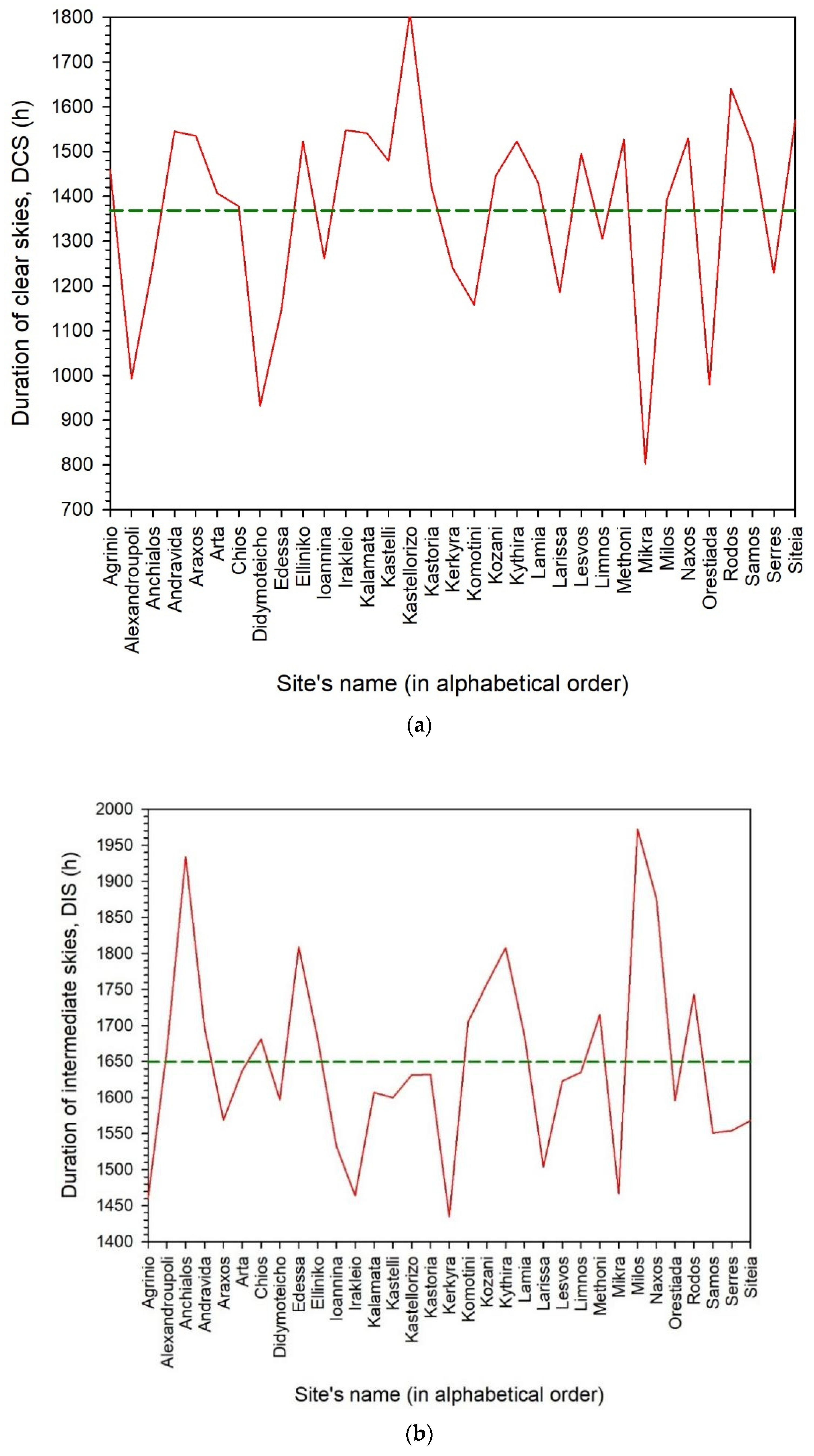
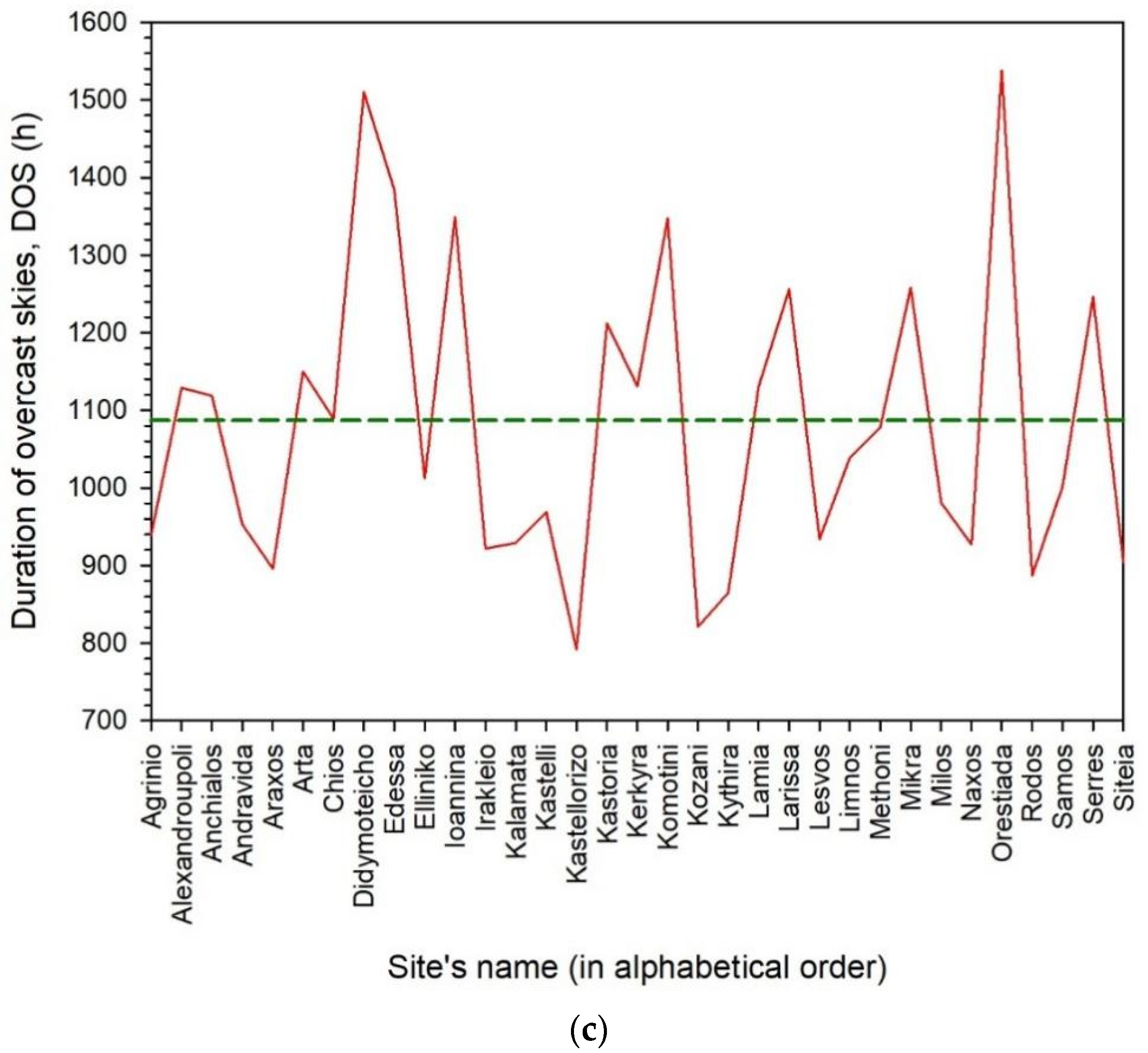
3.1. Annual Sky Status

Figure 2 depicts the annual hours across all 43 sites in Greece for the duration of clear skies (DCS), for intermediate skies (DIS), and for overcast ones (DOS). It is seen that the hour ranges for the three types of skies are [802 h, 1809 h], [1353 h, 1972 h], and [792 h, 1538 h] for DCS, DIS, and DOS, with average values of 1363.33 ± 219.54 h, 1647.27 ± 136.49 h, and 1083.76 ± 185.59 h, respectively. These results show that the intermediate-sky conditions over Greece prevail all over the year, followed by the clear-sky ones and then by the overcast situations. As the intermediate skies correspond to days with broken or fast-moving or low-level or cirrus clouds, it is implied that most of the time the weather conditions over the country favour this dynamic situation on an annual basis. Another interesting observation is the spread of the sky-condition hours as expressed by their standard deviations; the highest spread is for clear skies (219.54 h), followed by that for overcast (185.59 h), and then for intermediate (136.49 h). This observation dictates the conclusion of a wide-spread uniformity of dynamic weather conditions (e.g., fast-moving fronts) over Greece resulting in a sky status between clear and overcast. As far as the high standard deviation for the clear conditions is concerned, this may be due to the inhomogeneity of weather over Greece at the same time (e.g., overcast conditions in northern Greece, clear skies in the south).

Figure 3 is rather repetitive of Figure 2; in this case, the abscissa has been replaced with the geographical latitude of the sites in order to investigate its influence on sky conditions, as implied by the discrepancy in the standard deviations discussed above. Both linear and non-linear fits to the data points have been drawn in order to show their accuracy.

Table 1. Expression of the annual cases (in h) for clear, intermediate, and overcast skies over Greece as function of the geographical latitude (φ in degrees N) of the sites. The fits are linear and non-linear. R² = coefficient of determination; SEE = standard error of the estimate; ρ = Pearson correlation coefficient; MBE = mean bias error; RMSE = root mean square error. DCS (or SSD) = duration of clear skies (or sunshine duration, according to the WMO definition); DIS = duration of intermediate skies; DOS = duration of overcast skies (all durations in h). All regression fits are at the 95% confidence level (α = 0.05) and have been derived from the TMYs of the sites. The mathematical formulas for the statistical indicators and their interpretation are given in Appendix A.

Sky Conditions Regression Type	Regression Equation and Statistics
Clear skies Linear fit	SSD = DCS = −93.2462 × φ + 4957.8727 R2 = 0.6088, SEE = 139.1117 h ρ = 0.7802, MBE = 0.0007 h, RMSE = 135.8380 h
Clear skies Non-linear fit	$\mathrm{SSD} = \mathrm{DCS}=0.0314 \times \phi$6$- 7.7403 \times \phi$5$+ 788.9171 \times \phi$4$– 42,568.8275 \times \phi$3 + 1,283,$513.7786 \times \phi$2$– 20,516,430.9885 \times \phi$ + 135,895,710.1637 R2 = 0.6758, SEE = 135.1449 h ρ = −0.8017, MBE = −617.5914 h, RMSE = 734.5978 h
Intermediate skies Linear fit	DIS = −11.6328 × φ + 2097.1513 R2 = 0.0242, SEE = 137.3808 h ρ = 0.1557, MBE = −0.0006 h, RMSE = 134.1479 h
Intermediate skies Non-linear fit	$\mathrm{DIS} = 0.7466 \times \phi$6$- 171.7414 \times \phi$5$+ 16,447.7466 \times \phi$4$– 839,383.0735 \times \phi$3$+ 24,074,471.9759 \times \phi$2$– 367,933,208.7171 \times \phi$ + 2,340,906,375.2554 R2 = 0.1613, SEE = 135.9257 h ρ = −0.1815, MBE = 12.4862 h, RMSE = 496.1667 h
Overcast skies Linear fit	DOS = 77.5583 × φ − 1898.8673 R2 = 0.5840, SEE = 121.8230 h ρ = 0.7642, MBE ≈ 0.0000 h, RMSE = 118.9562 h
Overcast skies Non-linear fit	$\mathrm{DOS} = 0.9297 \times \phi$6$- 212.0317 \times \phi$5$+ 20,137.1181 \times \phi$4$– 1,019,440.4094 \times \phi$3$+ 29,014,851.7739 \times \phi$2$– 440,201,405.0524 \times \phi$ + 2,781,298,726.7945 R2 = 0.6972, SEE = 110.9131 h ρ = 0.7905, MBE = 172.4234 h, RMSE = 289.5424 h

gives the expression of the fits and some statistics; all fits are at a 95% confidence level. The following observations can be induced from the Figures.

(i)

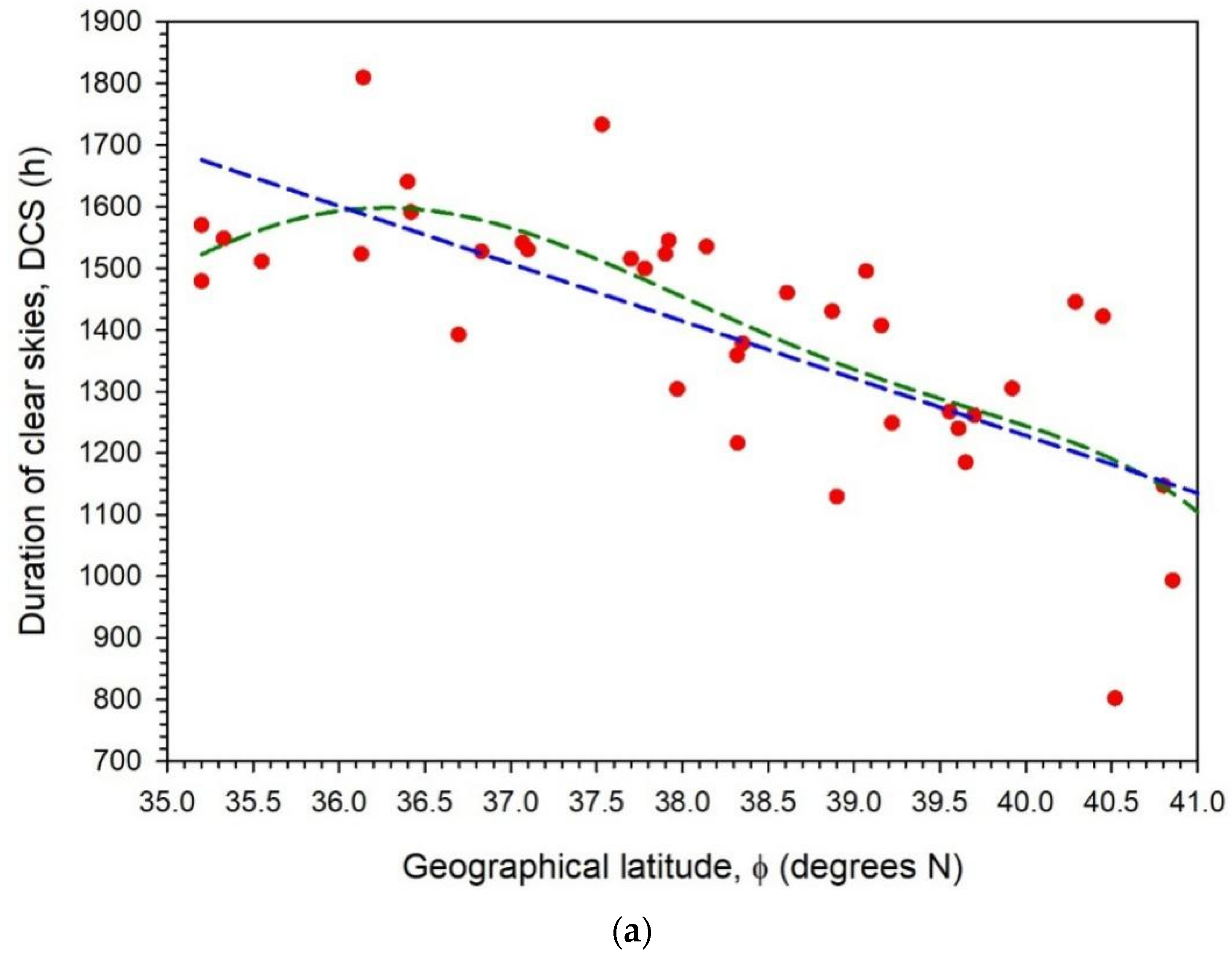
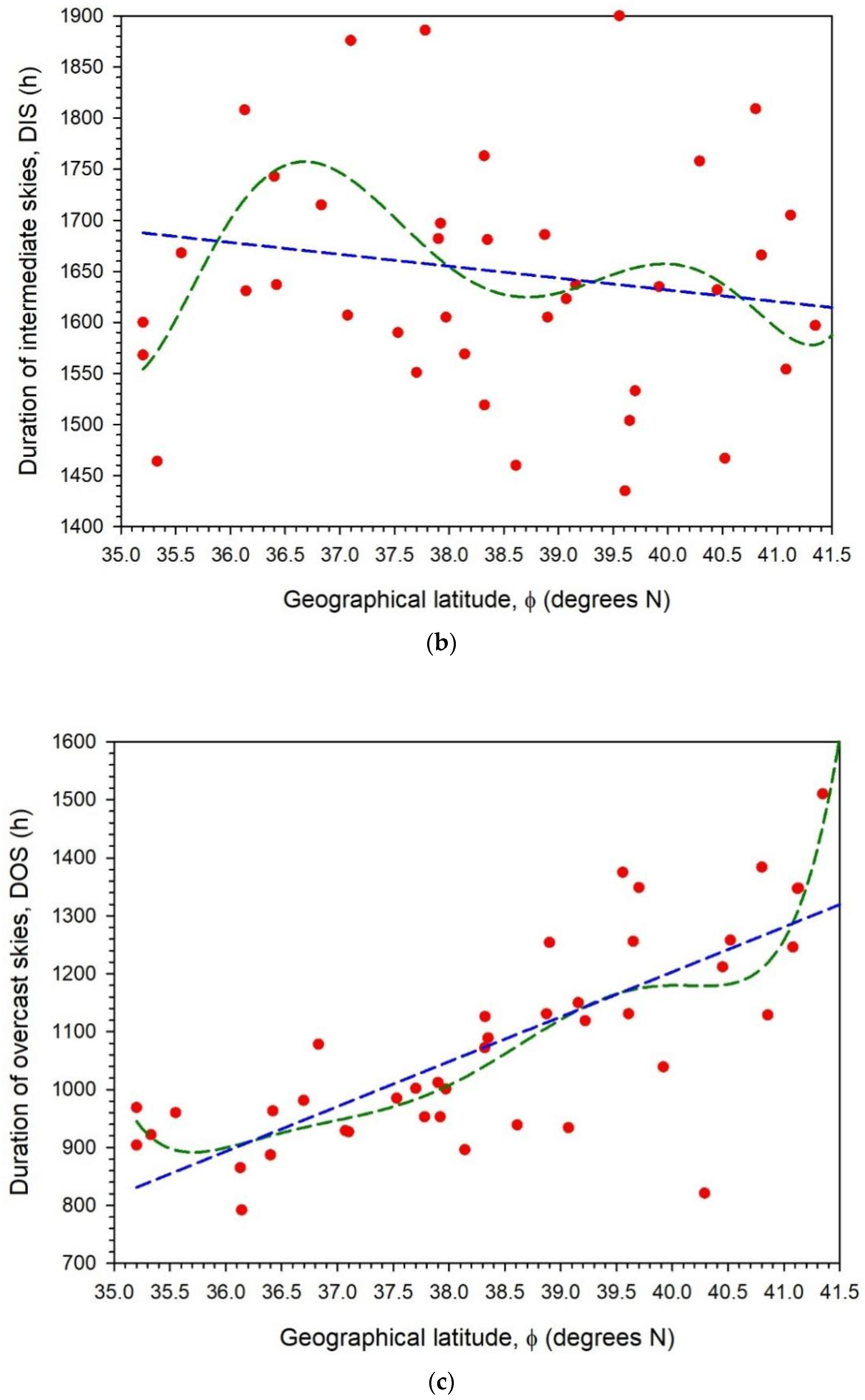
The accuracy of the estimates in the DIS case is much lower than that for the DCS or DOS ones; this visual observation is confirmed by the R² values in Table 1.

(ii)

The non-linear regression equations provide better fits to the data points; this result is confirmed by the higher R² values of the non-linear expressions in comparison to those for the linear equations.

(iii)

For the DCS and DOS cases, the linear fits are close to the non-linear ones (comparable R² values).

(iv)

The dispersion of the data points around the linear/non-linear regression lines is almost the same in any of the three sky types (consult the SEE values); this outcome shows that the choice of the selected regression equations gives the best possible results.

(v)

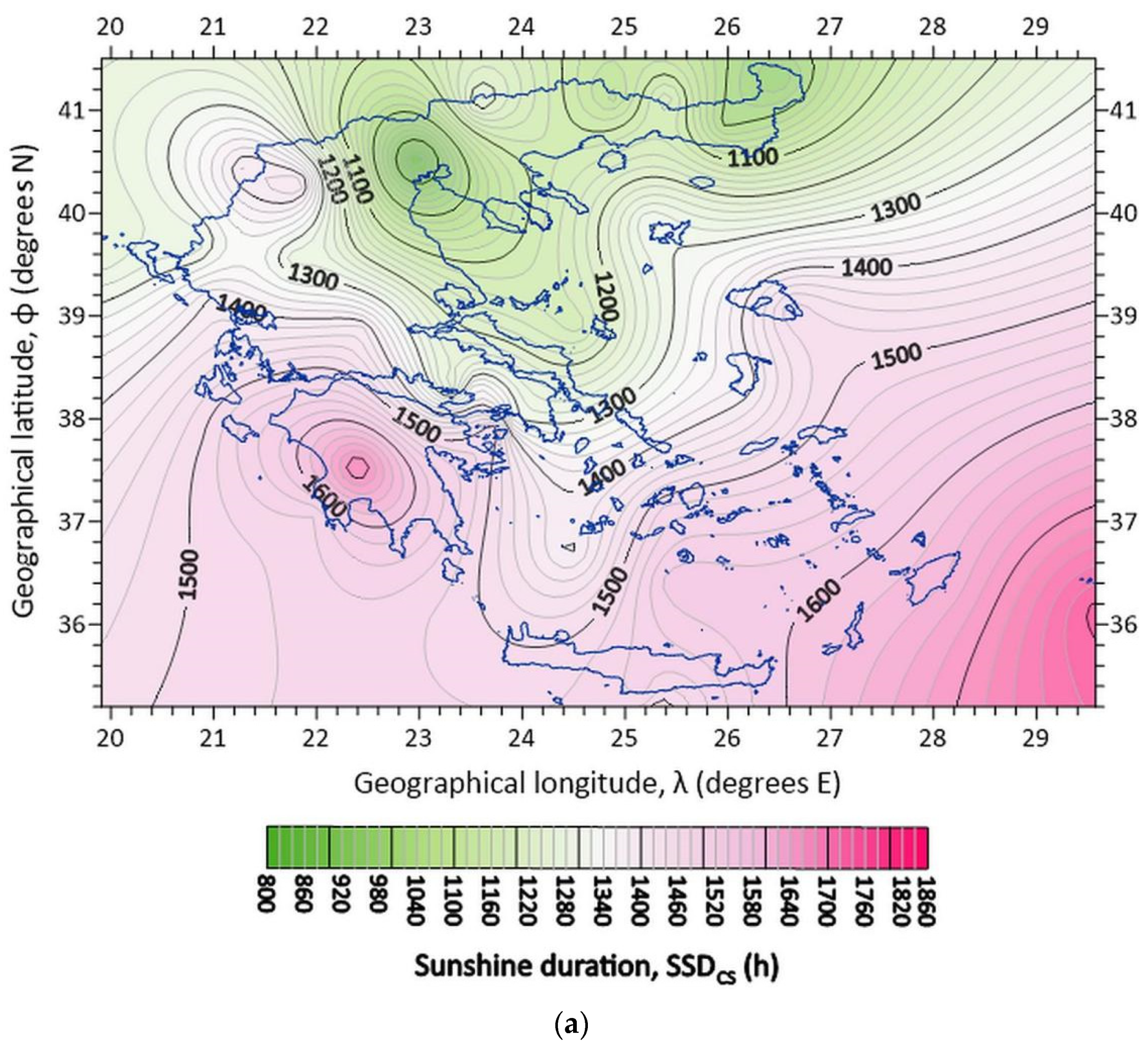
There is a strong/weaker decreasing trend in the duration of the DCS/DIS sky conditions with increasing φ.

(vi)

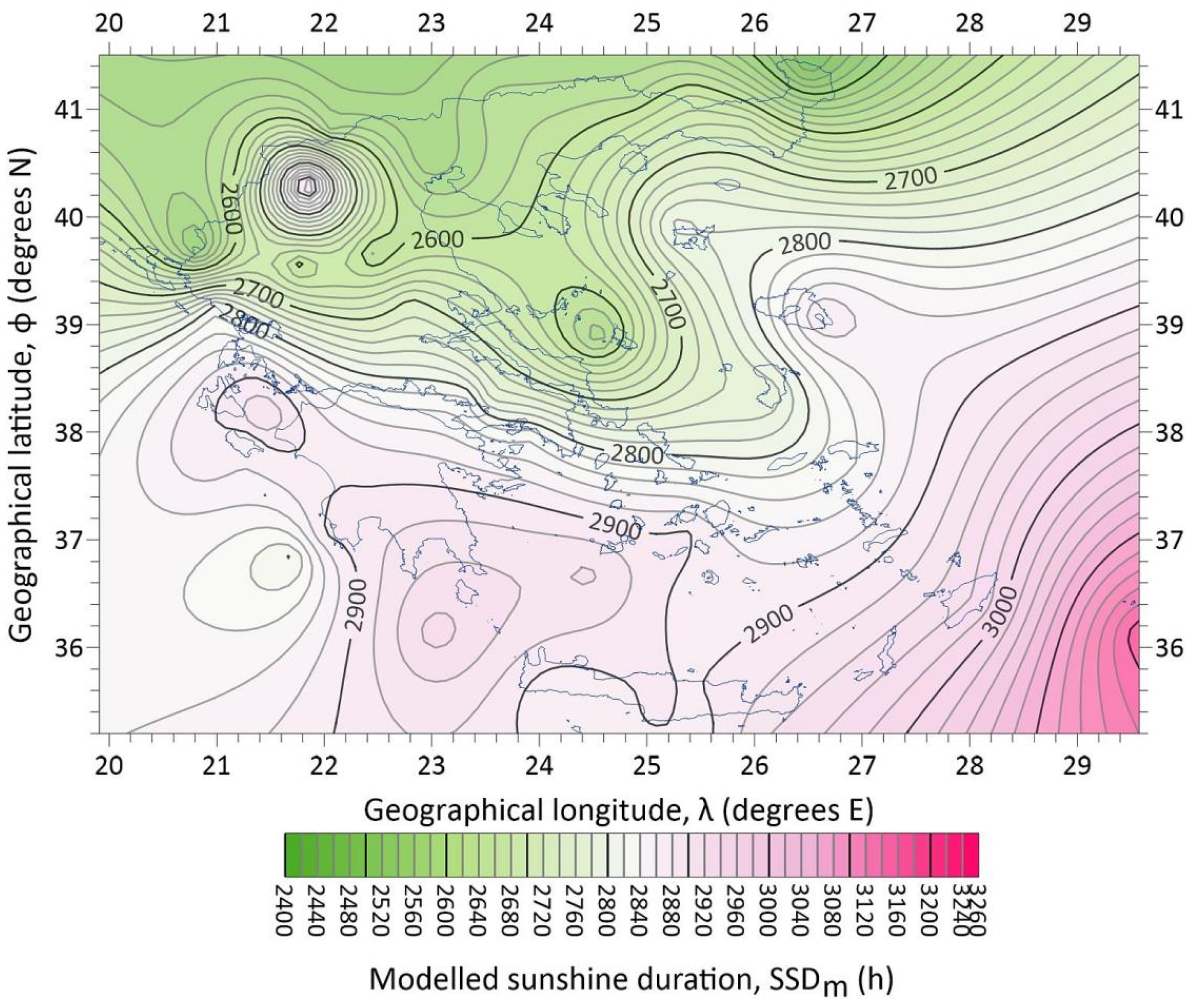
There is a positive trend in the DOS sky conditions with increasing φ; this is due to the prevalence of more cloudy weather as one moves from southern to northern Greece.

(vii)

There is a good correlation and a good anti-correlation between the observed and estimated values in the DCS case for the linear and non-linear fit, respectively, as shown by the ρ values in Table 1. Good positive correlation exists in both linear and non-linear models in the DOS case. On the contrary, the correlations in the DIS case are poor.

(viii)

The almost zero values of the MBEs in the linear fits to all sunshine duration cases imply an almost perfect match between estimated and observed values.

(ix)

The lower RMSE values for the linear regression lines in all sunshine duration cases show that the estimates are more concentrated around their linear regression lines than the non-linear ones.

Some general outcomes from the above comments are that the SEE values in all 3 types of sky conditions and both regression fits are comparable; this means that the accuracy of the estimates around the regression lines is the same in all cases, no matter whether there is a poor R² (as in DIS). Moreover, the linear regression lines seem to do the job of approaching the observed values more adequately than the non-linear ones, since their MBEs are almost equal to zero (no over- or under-estimation exists). This is further confirmed by the comparable RMSE values for the linear fits, a fact that implies comparable dispersion (spread) of the estimated values around the linear curves.

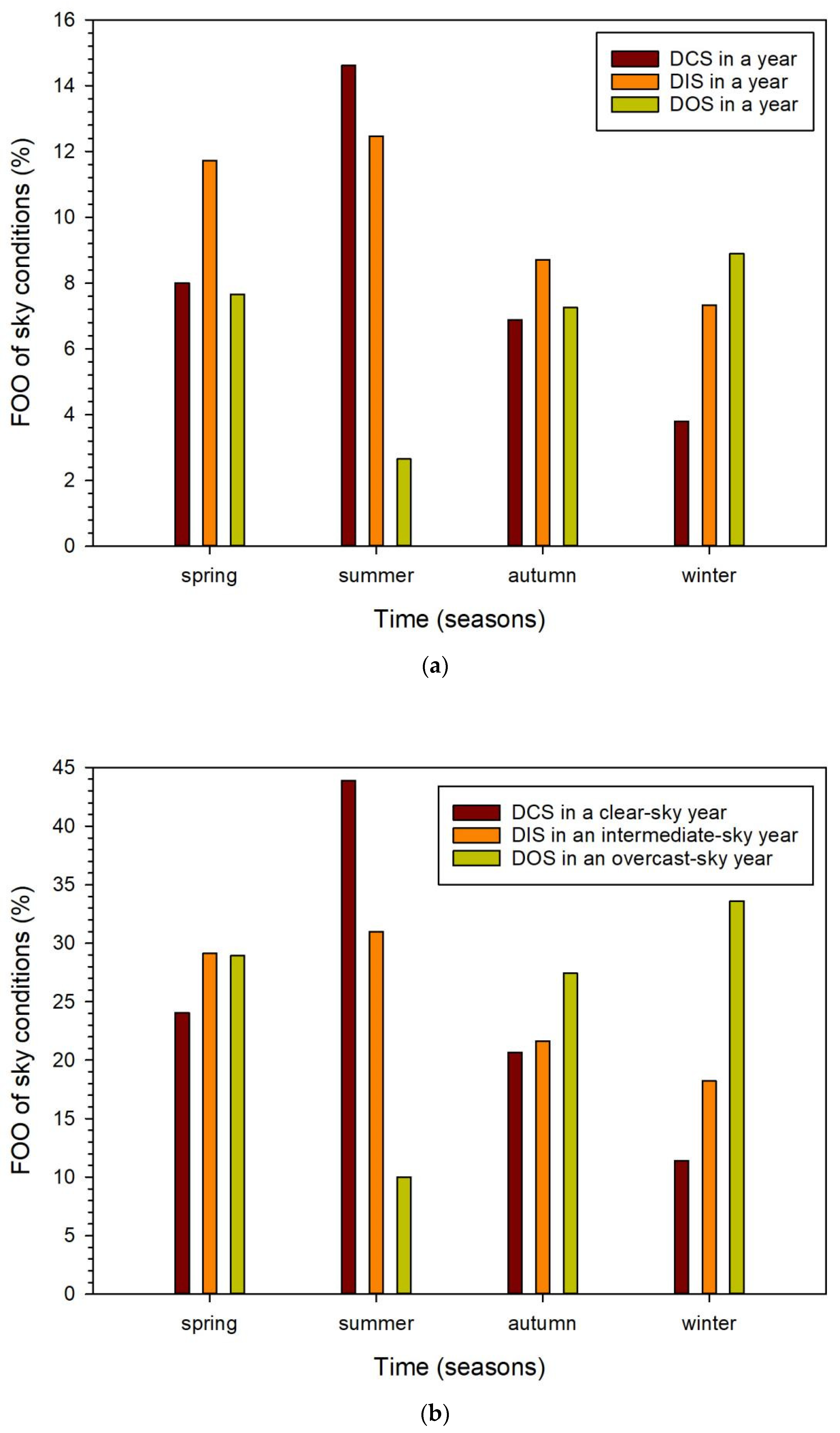
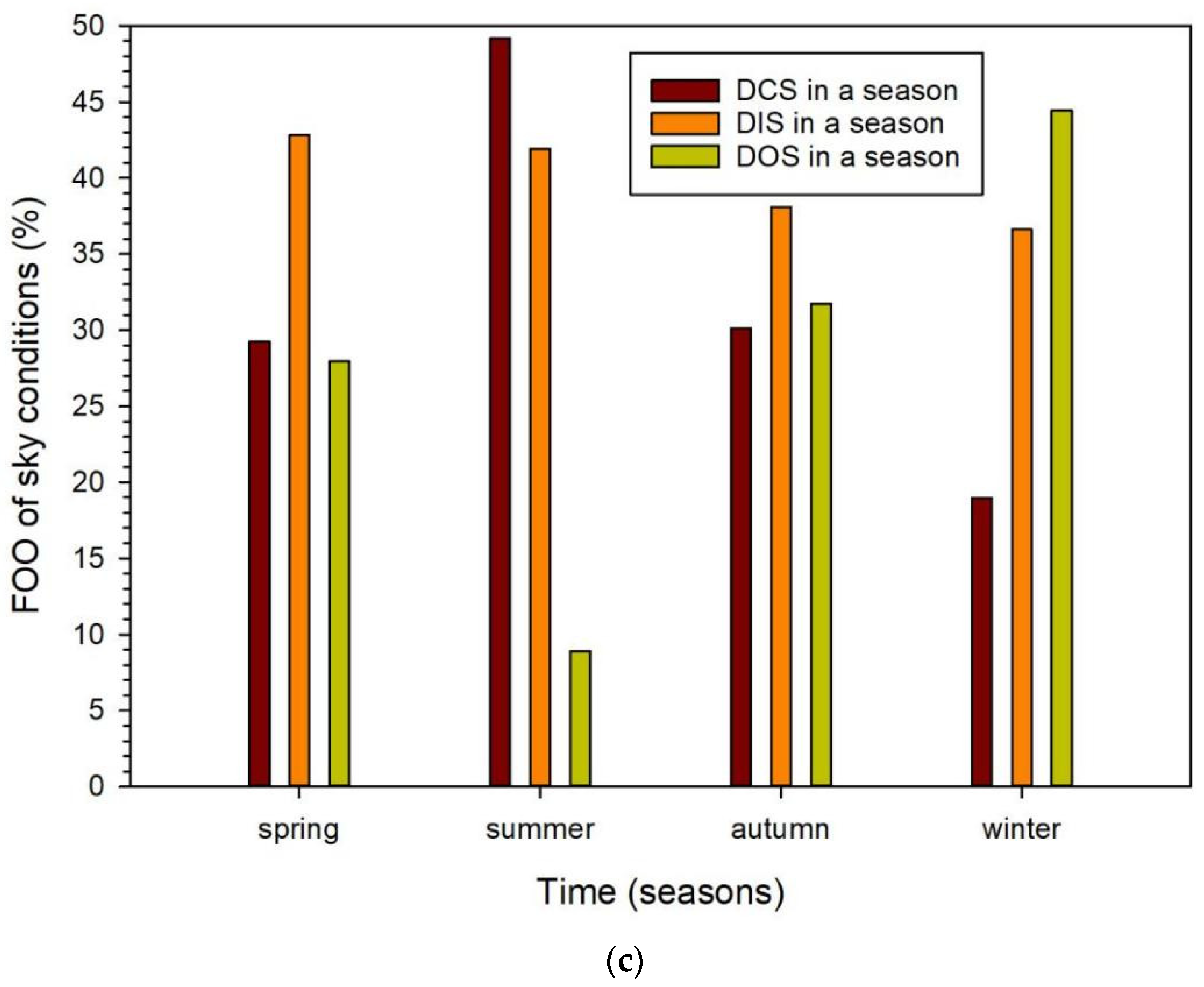
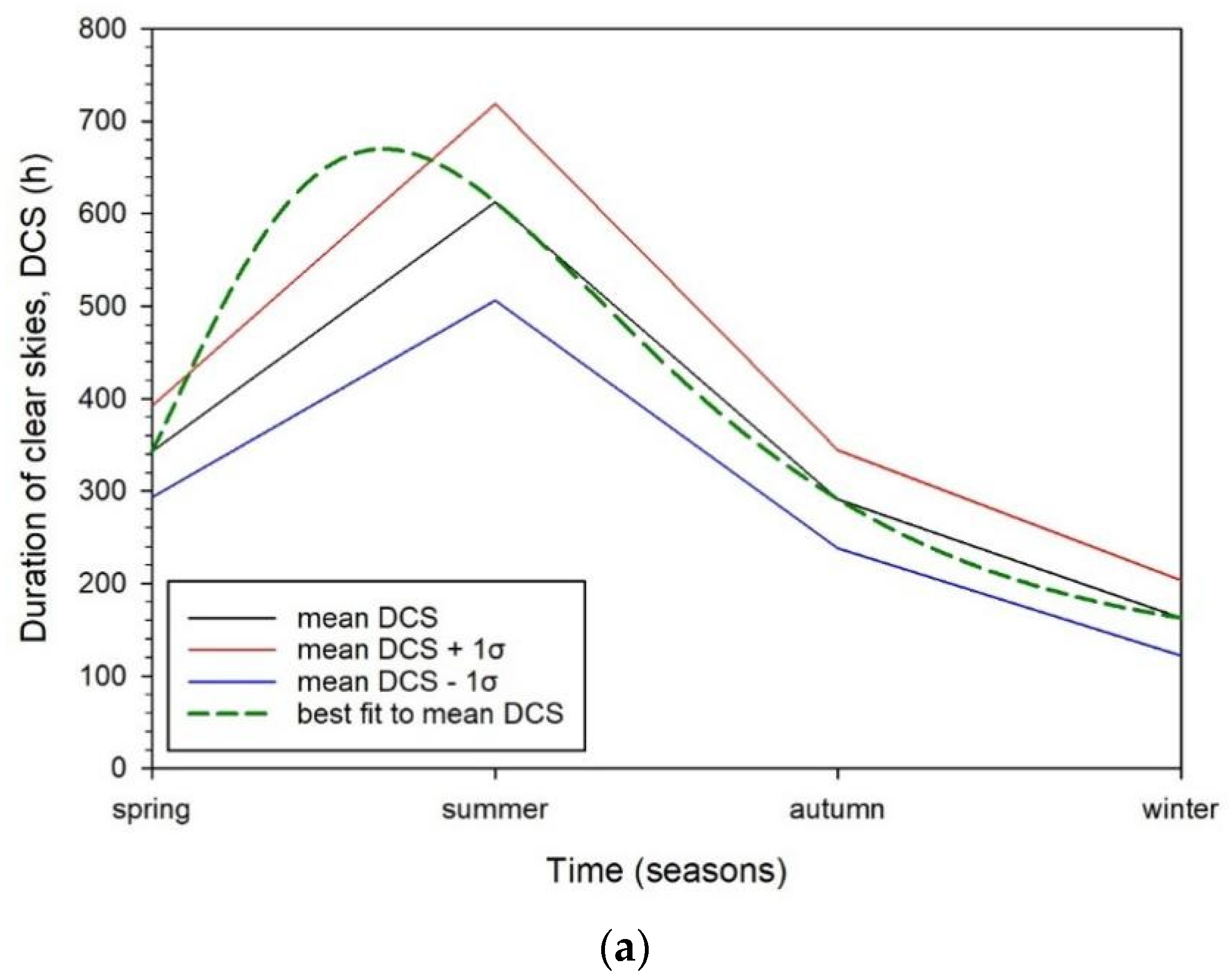
3.2. Seasonal Sky Status

This section provides an analysis of the sky conditions over Greece on a seasonal basis. For clarity, spring includes March, April, and May; summer consists of June, July, and August; autumn has the months of September, October, and November; and winter contains December, January, and February. Figure 4 give the frequency of occurrence (FOO, in %) for the duration of all three types of sky conditions (clear, intermediate, overcast, as defined in Section 2.2). Figure 4a represents the time occupied by DCS, DIS, or DOS conditions in a TMY. The sum of all percentages shown by the bars in the figure gives 100% (corresponding to 4108 h annually). The DCS and DIS conditions show a maximum in the summer season, while the opposite occurs for the DOS cases. The DIS conditions are favoured in spring (a transition season from winter to summer), while the DCSs prevail in summertime, as expected. Figure 4b depicts the FOOs for the DCS, DIS, and DOS conditions within the TMY. The sum of all FOOs in the same season is 100% (4108 h annually). The occurrence of DCSs is highest in the summer, while the DISs and DOSs have equal percentage occurrence in spring (transition season). The pattern of Figure 4a is repeated in Figure 4b, i.e., higher frequencies for the DCS and DIS skies in the summer and lower for the DOS ones; the DOSs are highest in winter, as expected. Figure 4c gives the frequencies for the DCS, DIS, and DOS events within the same season. It is seen that spring is dominated by DIS skies (transition period), summer by DCS cases (expected), autumn by DIS events (transition period), and winter by DOS skies (expected). The sum of the percentages within any season gives 100% (i.e., 4108 h annually = 1125 h for spring + 1221 h for summer + 939 h for autumn + 823 h for winter).

Figure 5 show the seasonal mean DCS, DIS, and DOS values together with the ±1σ band. Best-fitted curves are also shown by the green dashed curves. Though the regression lines come out of the ±1σ band (σ = standard deviation) between the spring and summer mean values, they go exactly through the seasonal values; this gives them an R² = 1. The expressions of the regression lines are given in

Table 2. Expression of the seasonal mean duration (in h) for the clear, intermediate, and overcast skies from the TMYs of the 43 sites as function of the season, t, in the range [1 (spring), 4 (winter)]. R² = coefficient of determination; SEE = standard error of the estimate. SSD/DCS = sunshine duration/duration of clear skies; DIS = duration of intermediate skies; DOS = duration of overcast skies (all durations in h). All regression fits are at the 95% confidence level (α).

Sky Conditions	Regression Equation and Statistics
Clear	SSD = DCS = 983.0168 × exp{−0.5 × [ln(t/1.9320)/0.3804]2/t} R2 = 1, SEE = 0 h, α = 0.05
Intermediate	DIS = 968.7578 × exp{−0.5 × [ln(t/1.9336)/0.3855]2/t} R2 = 1, SEE = 0 h, α = 0.05
Overcast	$\mathrm{DOS} = 289.0910 \times (t^{-90.3392\times t^{-6.1013}}$) R2 = 0.9993, SEE = 3.6101 h, α = 0.05

. As also shown by Figure 5, the higher seasonal durations of the sky conditions over Greece during the summer are the DCS and DIS cases; the opposite exists for the DOS occurrences.

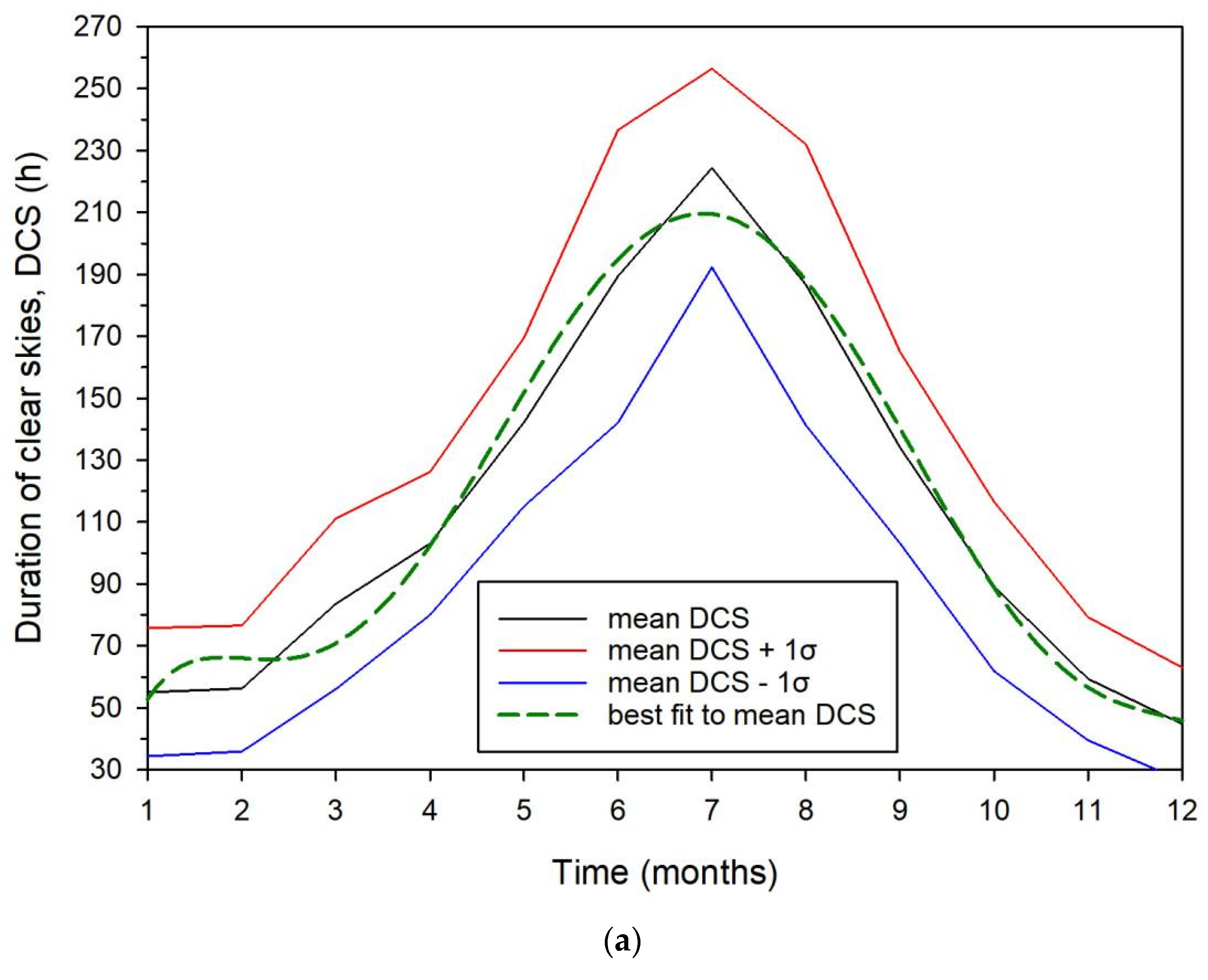
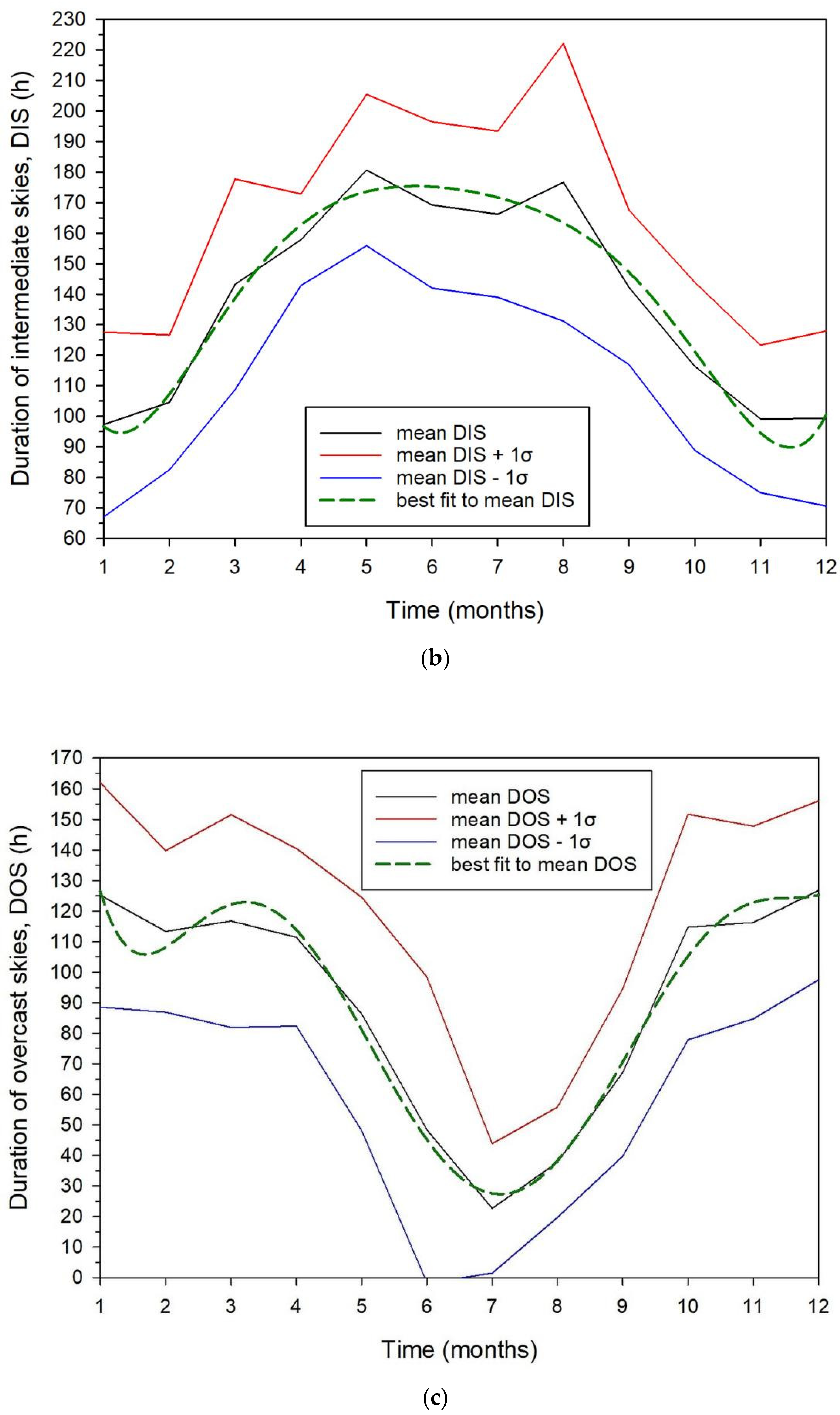
3.3. Intra-Annual Sky Status

The present section provides an analysis of the sky conditions over Greece on a monthly basis. Figure 6 shows the monthly mean values of the duration of sky conditions (DCS, DIS, DOS) with the ±1σ band and the best-fitted curves to the mean ones at the confidence level of 95%. More particularly, Figure 6a depicts a smooth intra-annual variation in the DCS (or else SSD) with its maximum in July and its minimum values during winter, as expected. The best-fitted regression curve to the mean DCS values lies within the ±1σ, a fact that implies 95% of the DCS events are fully described by the fitted curve. Figure 6b shows the intra-annual variation of the DIS conditions over Greece; two local maxima are found, one in May and another in August. The first maximum appears in spring time (transition season), while the second is due to the frequent thermal storms of short duration in early afternoon at near-shore areas because of temperature differences between land and water [36]. Figure 6c presents the intra-annual variation in the DOS cases over Greece; lowest values in the summer and highest in winter occur, as expected.

Table 3. Non-linear expressions of the monthly mean duration (in h) for the clear, intermediate, and overcast skies from the TMYs of the 43 sites as function of the month (t), with t ∈ [1, 12]. R² = coefficient of determination; SEE = standard error of the estimate. SSD/DCS = sunshine duration/duration of clear skies; DIS = duration of intermediate skies; DOS = duration of overcast skies. All regression fits are at the 95% confidence level (α).

Sky Conditions	Regression Equation and Statistics
Clear	$\mathrm{SSD} = \mathrm{DCS} = -0.0110 \times t$6 + 0.4560 × t5 − 7.1042 × t4 + 51.0454 × t3 − 170.5219 × t2 + 260.5100 × t − 81.5485 R2 = 0.9838, SEE = 11.4553 h, α = 0.05
Intermediate	$\mathrm{DIS} = 0.0063 \times t$6 − 0.2435 × t5 + 3.7120 × t4 − 28.1920 × t3 + 106.7279 × t2 − 160.6950 × t + 175.3897 R2 = 0.9648, SEE = 9.0997 h, α = 0.05
Overcast	DOS = 0.0119 × t6 − 0.5002 × t5 + 8.0436 × t4 − 61.1764 × t3 + 223.5341 × t2 − 366.5001 × t + 323.0779 R2 = 0.9820, SEE = 7.3930 h, α = 0.05

presents the regression polynomials of the fitted curves to the monthly mean duration of sky conditions as function of the month; all of them are sixth-order polynomials. It is worth observing the high R² values (accuracy of the estimated regression curves) and the decreasing SEE values (dispersion of the monthly data around the regression curves) from clear to overcast skies. The latter outcome is due to the following reason: the k_du and k_dl limits mentioned in Section 2.2 (step 5) are not clear-cut ones, meaning that there may be an “intrusion” of DSC events registered as DIS, “intrusion” of DIS occurrences into the DCS and DOS zones, and “intrusion” of DOS events into the DIS band. It is apparent that the DCS data may be “disturbed” from the intrusion of some DIS events. To the contrary, the DIS data are more insensitive to an intrusion of some DCS or DOS cases because the sky, in this case, is partially covered by clouds. Finally, the DOS data do not respond to an intrusion of DIS events because the sky is fully covered in this case. The same explanation applies to the SEE values of Table 1. More about this “intrusion” rationale is given in Section 5.

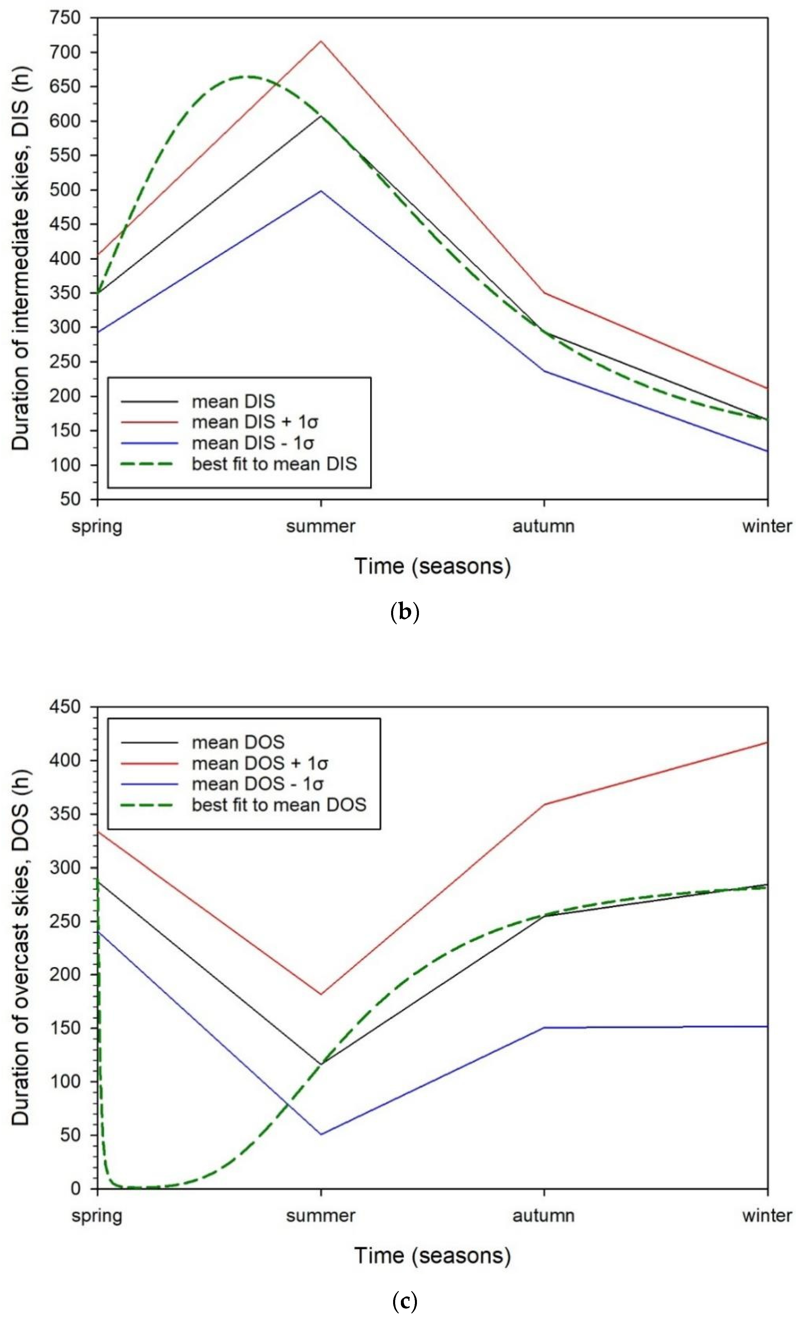
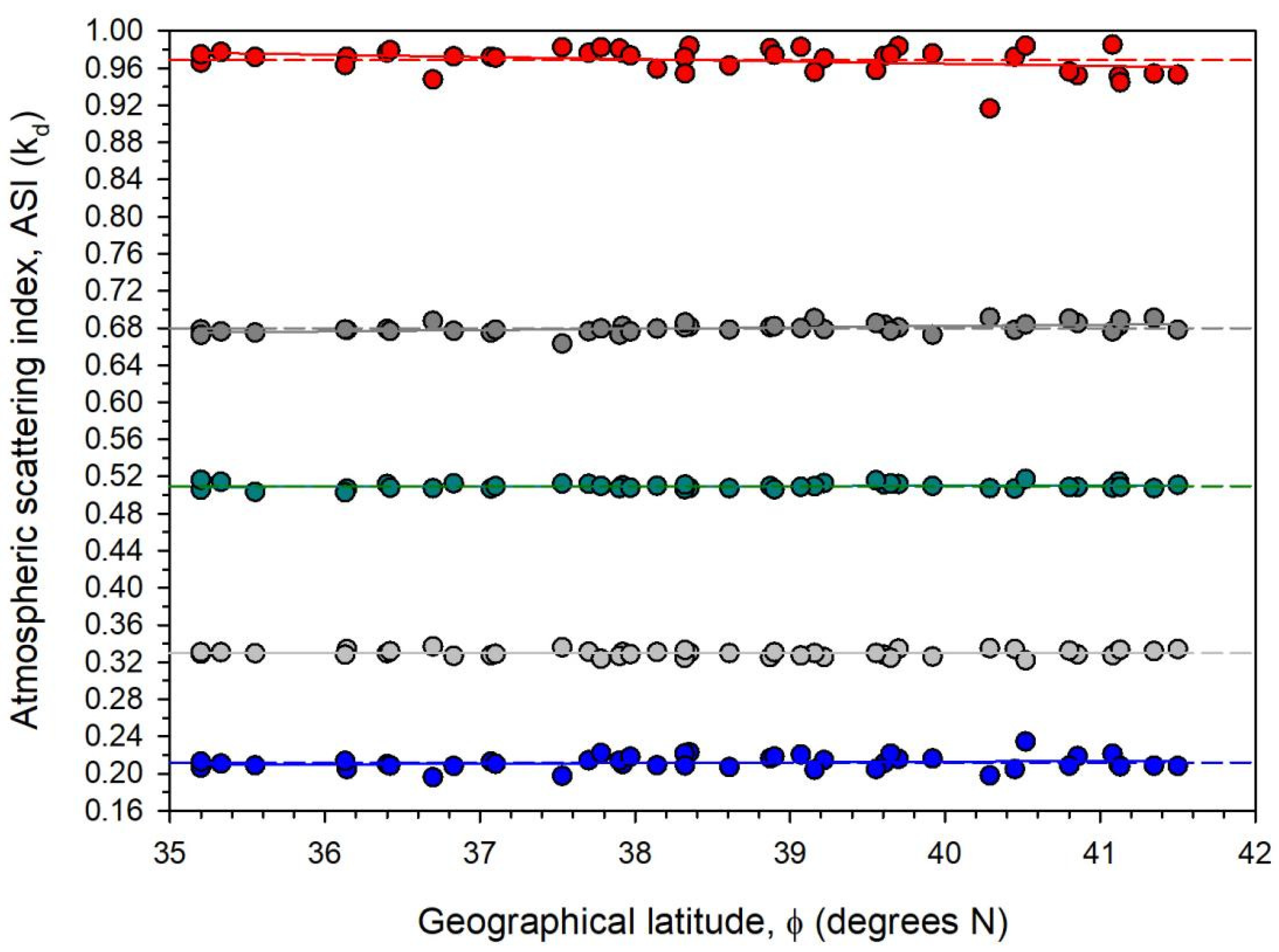
3.4. Sunshine Duration and Atmospheric Scattering

This section is focused on these two parameters, as indicated by the title of the article. As far as the sunshine duration is concerned, this coincides with the DCS events, as shown in the previous sections. Therefore, no further discussion is needed to be made. This gives some space for the second parameter.

Kambezidis [23] has presented an interpretation of k_d as an ASI and used it as such. The count of the hourly k_d values within the posed limits mentioned in step 5, Section 2.2, actually corresponds to the DCS, DIS, and DOS events (i.e., hours) at all sites in their respective TMYs, as already explained previously. In this context, by using the notion of k_d as ASI, one could interpret the results presented so far as atmospheric scattering (AS) under clear-, intermediate-, and overcast-sky conditions. Having this in mind, the distribution of the three types of AS over Greece on annual basis is 33% for AS_CS (subscript CS for clear skies), 40% for AS_IS (subscript IS for intermediate skies), and 27% for AS_OS (subscript OS for overcast skies). It is seen that greater AS is caused by intermediate-sky conditions followed by clear and overcast skies. This may look fallacious at first glance, as one would expect that AS should increase with the presence of more clouds (i.e., DOS cases). In fact, the scattering mechanism depends on the type of clouds and the cloud cover of the sky, as well as their altitude. Liou [37] claims that:

• Thick clouds (nimbostratus, cumulonimbus) reflect 80–90% of the incident solar light (in the 300–3000 nm spectrum) back to space, while they absorb just 10–20% of it;
• Fair weather cumulus clouds reflect and absorb 68–85% and 4–9%, respectively; they scatter to the surface the remaining solar flux, accounting for 15–32%;
• Thin stratus clouds reflect and absorb 45–72% and 1–6%, respectively, of the solar flux, while they scatter 28–55% to the surface;
• For alto-stratus clouds, these figures are 57–77% and 8–15%, respectively, while the scattering to the surface of the Earth constitutes 23–43%;
• The absorption mechanism is triggered in the near-infrared band of the solar spectrum, i.e., for wavelengths longer than 700 nm.

The above conclusions have not taken into account the scattering mechanism by air molecules and atmospheric aerosols, which contribute to the mechanism [38]. If both factors (clouds and aerosols) are considered, then one can justify the results of the occurrence of AS_CS, AS_IS, and AS_OS shown above as follows:

• In clear-sky conditions, scattering of solar light is only due to atmospheric aerosols (natural or anthropogenic) and in certain fair-weather cases to cumulus clouds; this occurs for 33% of the time in a year over Greece;
• In intermediate-sky conditions, when a variety of clouds (cumulus, stratus, cirrus) may be present in the sky at different instances in a year, aided by the presence of atmospheric aerosols, the scattering of solar light occupies more time in a year (40%);
• In overcast-sky conditions, scattering to the surface of the Earth is least as the major part of the incident solar flux is reflected to space; this gives a figure of 27% of the time in a year over Greece.

In order to investigate AS further, an additional subdivision of the k_d limits for intermediate skies is employed here for the first time worldwide. Three new ranges are defined: (i) intermediate-1-sky conditions for 0.26 < k_d ≤ 0.43 (i.e., presence of cirrus clouds with a clear-sky look), (ii) intermediate-2-sky conditions for 0.43 < k_d ≤ 0.60 (i.e., mix of clear skies with broken or fast-moving clouds [39,40]), and (iii) intermediate-3-sky conditions for 0.60 < k_d ≤ 0.78 (i.e., prevailing broken clouds with a more permanent character). Taking into account this subdivision of the k_d intermediate-sky range, the values of the scattering index for all 43 sites can be related to the geographical latitude of the sites, as firstly depicted in Figure 9 of [23] showing a linear dependence for clear- and all-sky conditions. Figure 7 repeats this linear dependence of ASI (i.e., of k_d) on φ for the k_d ranges corresponding to clear, intermediate-1, intermediate-2, intermediate-3, and overcast skies; the delimitation of k_d for the clear and overcast cases has been figured in step 5, Section 2.2. From Figure 7, it is seen that the linear regression curves coincide with the average lines in all cases except for the overcast skies. Indeed, this observation is confirmed in

Table 4. Linear expressions for the annual mean ASI for clear; intermediate-1, -2, -3; and overcast skies over Greece as function of the geographical latitude (φ in degrees N), of the sites in the range (35°, 42°). The ASI values are averages over the 43 sites from their TMYs. Ave = annual mean; R² = coefficient of determination; SEE = standard error of the estimate. The subscripts CS; IS-1, -2, -3; and OS to ASI denote clear; intermediate-1, -2, -3; and overcast skies, respectively. All regression fits are at the 95% confidence level (α).

Sky Conditions	Regression Equation and Statistics
Clear	ASICS = 0.0007 × φ + 0.1834 Ave = 0.2118, R2 = 0.0330, SEE = 0.0074, α = 0.05
Intermediate-1	${\mathrm{ASI}}_{\mathrm{IS}-1} = 2.5292 \times {10}^{-5} \times \phi$ + 0.3287 Ave = 0.3297, R2 = 0.0002, SEE = 0.0035, α = 0.05
Intermediate-2	ASIIS-2 = 0.0002 × φ + 0.4999 Ave = 0.5095, R2 = 0.0206, SEE = 0.0032, α = 0.05
Intermediate-3	${\mathrm{ASI}}_{\mathrm{IS}-3} = 0.0014 \times \phi$ + 0.6243 Ave = 0.6801, R2 = 0.2243, SEE = 0.0050, α = 0.05
Overcast	${\mathrm{ASI}}_{\mathrm{OS}} = -0.0024 \times \phi$ + 1.0613 Ave = 0.9685, R2 = 0.1018, SEE = 0.0133, α = 0.05

, where the constant terms in all linear equations are almost equal to the ASI average values. In all cases, the coefficients of φ are positive, except for the OS case, where it has a negative sign; nevertheless, all the constant terms have extremely low values, meaning that the fitted (solid) curves are almost parallel to the x-axis (i.e., they almost coincide with the horizontal average dashed lines); a slight deviation may, however, be observed in the case of the OS skies. All R² values are very low, a fact that implies a loose fit to the data points. On the other hand, the SEE values are two orders (one order for OS) of magnitude lower than the ASI values themselves, thus drawing the conclusion of very low dispersion of the data points around the regression lines.

3.5. Credibility of Results

To ensure that the DCS, DIS, and DOS results are acceptable, comparison of all-sky events with measured or modelled ones must take place. All 43 selected sites correspond to meteorological stations belonging to the HNMS network. However, the HNMS has not yet provided SSD-accredited data for the period 2007–2016 (from which period the TMYs have been derived in the PV-GIS platform). To overcome this difficulty, use of the free Global Climate Data of the German Weather Service (DWD) was made from the Climate Data Centre (CDC) of the German Weather Service (DWD)—Climate-ADAPT (europa.eu, accessed on 13 June 2022) platform; yearly sunshine durations were downloaded for the available Elliniko, Irakleio, Kerkyra, and Larissa sites in the period 2007–2016. In addition, measured SSD data from the Institute of Applied Physics, Academy of Sciences of Moldova (ASM) at Chisinau, were used for the period 2007–2015. SSD averages from the five sites were computed and are compared with the annual ones estimated in this work.

Table 5. Annual mean values of SSD for 4 sites from DWD (2007–2016), 1 site from ASM (2007–2015), and DCS from the TMYs of the sites. The fourth column presents the difference in the values from the three sources.

Site	SSD, External Source (h)	DCS, This Work (h)	SSD—DCS (h)
Chisinau, ASM	2346	1213	1132
Elliniko, DWD	2909	1523	1386
Irakleio, DWD	2905	1548	1357
Kerkyra, DWD	2593	1240	1353
Larissa, DWD	2435	1185	1250

shows this comparison. It is seen that large differences exist between the SSD values from the three sources (fourth column in Table 5). This outcome may be attributed to the fact that some k_d values though classified as DIS may have DCS characteristics. This issue is discussed in the following paragraph.

In order to investigate the above findings further, one might consider the sub-division of the IS cases into IS-1, -2, and -3 sky conditions, as mentioned in Section 3.4. This is performed because of a possible “intrusion” of k_d-DIS values into the k_d-DCS range. To limit this intrusion and make things clearer, consideration of the DIS-1, DIS-2, and DIS-3 sub-ranges was taken into account. These sub-ranges correspond to k_d ∈ (0.26, 0.43) for DIS-1, to k_d ∈ (0.43, 0.60) for DIS-2, to k_d ∈ (0.60, 0.78) and were defined as to have equal k_d lengths, i.e., 0.17, 0.17, and 0.18, respectively, for DIS-1, DIS-2, DIS-3. It is now assumed (without experimental justification) that the clear-sky hours in the DCS band obtain intrusion from all three DIS sub-ranges in a weighted manner; therefore, a new formula is proposed for estimating (approximating) the real SSDs: SSD_m = DCS + DIS-1 + 0.8 × DIS-2 + 0.5 × DIS-3. According to this assumption,

Table 6. Annual mean values of SSD from DWD, ASM, and DCS, DIS-1, -2, -3 from this work. The difference in the last column is expressed as SSD − SSD_m = SSD − (DCS + DIS-1 + 0.8 × DIS-2 + 0.5 × DIS-3) for the five sites of Table 5. DIS-1 corresponds to the k_d counts in the interval (0.26, 0.43], DIS-2 to (0.43, 0.60], and DIS-3 to (0.60, 0.78].

Site	SSD (h)	DCS (h)	DIS-1 (h)	DIS-2 (h)	DIS-3 (h)	Difference (h)
Chisinau, ASM	2346	1203	778	511	0	−71.1
Elliniko, DWD	2905	1523	813	481	239	64.7
Irakleio, DWD	2905	1548	804	506	297	−0.3
Kerkyra, DWD	2593	1240	892	462	351	−84.1
Larissa, DWD	2435	1185	864	495	264	−142

provides the new differences between the SSD-DWD and SSD-ASM sources and the above aggregation for each of the five sites in Table 5. It is seen that the differences have now improved, i.e., decreased dramatically. Nevertheless, this assumption must be verified in the future against sunshine-duration measurements for more sites of the HNMS network or elsewhere in the world. On the other hand, one should not forget that the k_d values in all ranges and sub-ranges can be attributed to equivalent ASI ones. The rationale for developing the above-mentioned model is explained in detail in Section 5.

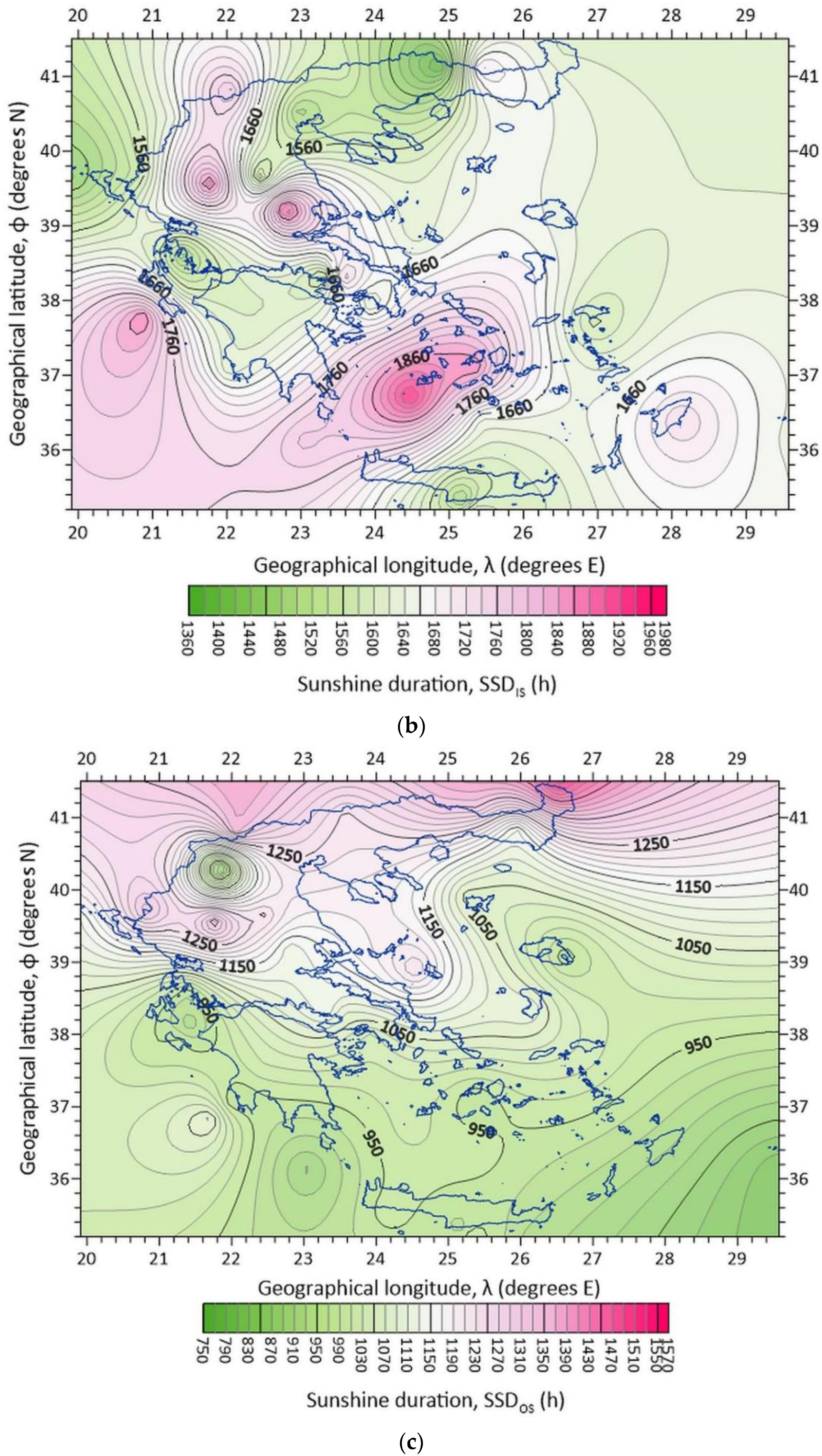
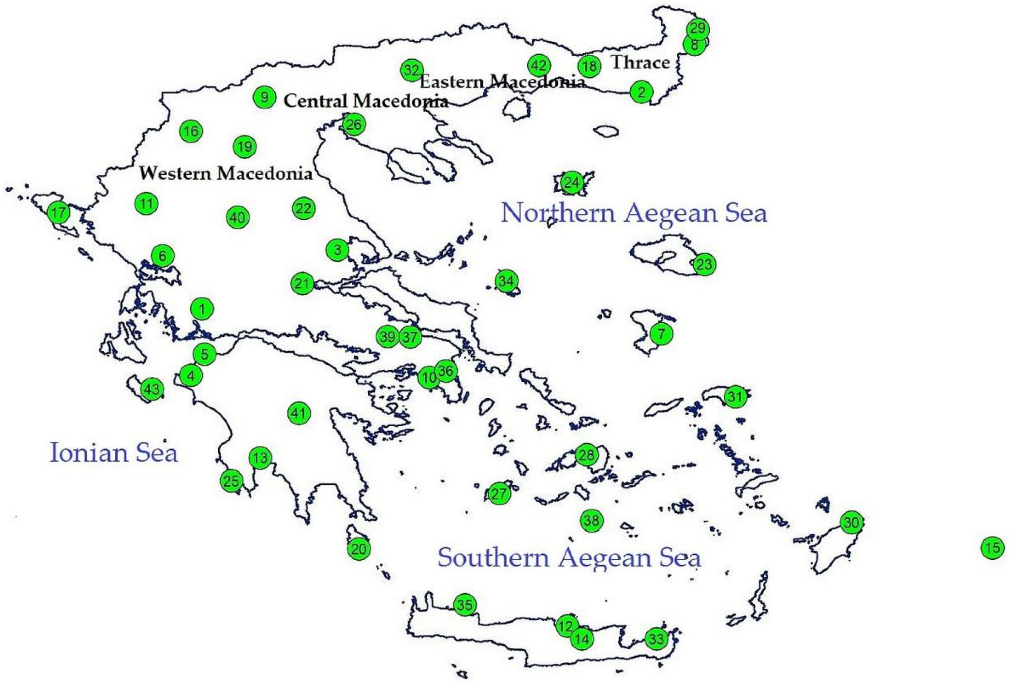
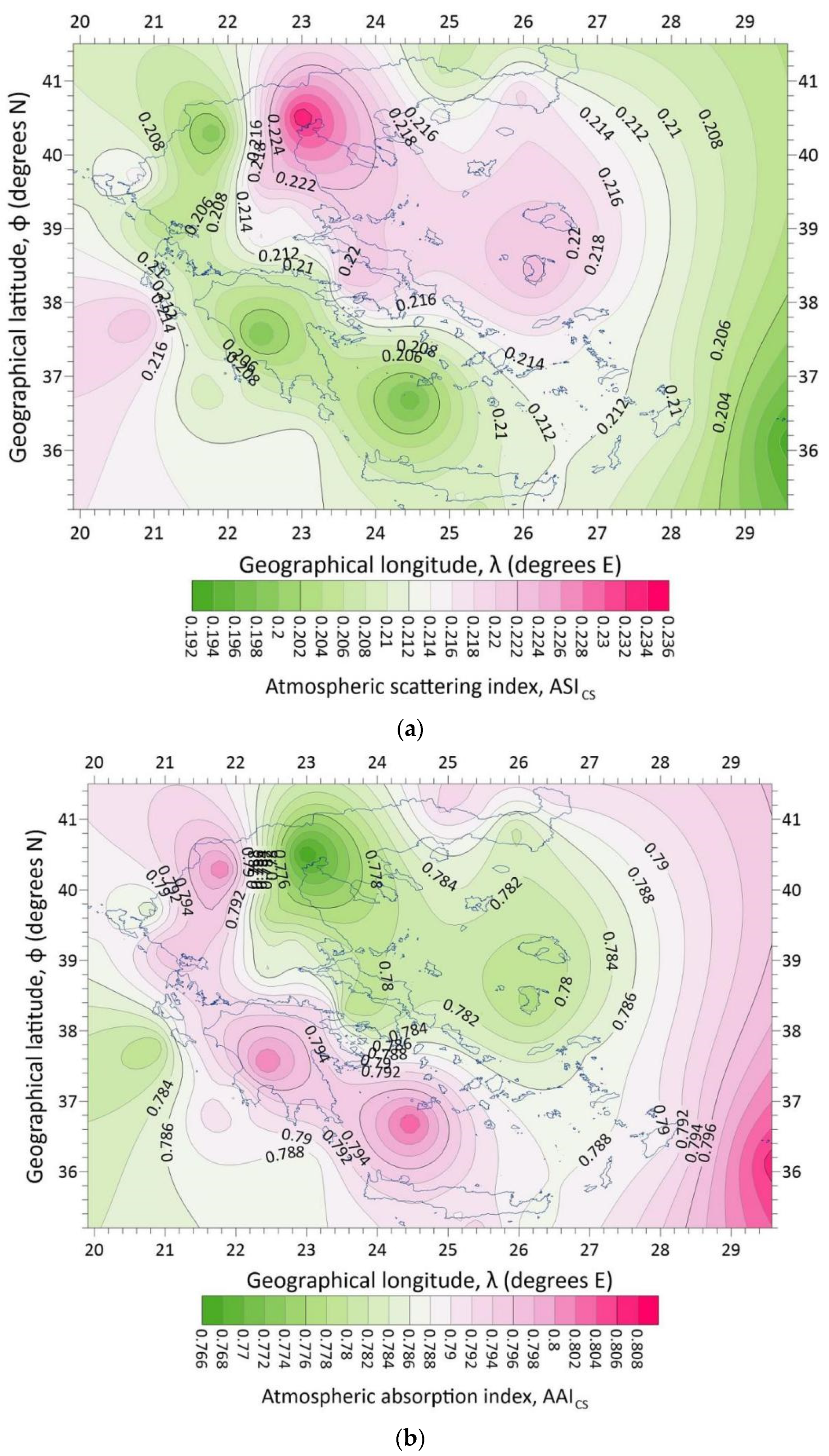
3.6. Annual Maps of Sky Status

This section is devoted to the depiction of the dispersion of the sky conditions over Greece. Indeed, Figure 8 show the distribution of the clear-, intermediate-, and overcast-sky events as annual values of the TMYs across the 43 sites. Figure 8a shows the distribution of the clear-sky conditions over Greece. It is apparent that higher SSD values occur in the southern part of Greece, i.e., below the geographical latitude of 39°. In other words, the country can be divided into two parts, northern and southern as far as SSD is concerned. The pattern for overcast skies in Figure 8c presents an opposite pattern to that for clear skies, i.e., greater number of sunshine hours in the northern part of Greece in comparison with that for the southern half; this is in agreement with the regression curve for the DOS cases shown in Table 4: decreasing ASI with latitude results in cleaner atmosphere, which permits more solar radiation to reach the surface. The pattern for intermediate-sky conditions is shown to be between those for clear and overcast conditions. Higher DIS values occur in the southern Aegean and southern Ionian Seas with secondary peaks over central and north-western Greece. In viewing these results as ASI, one can refer to the map of Figure 11a in [41], where the solar flux on flat-plate surfaces tilted at 25–30° to south presents exactly the same pattern with that of Figure 8a of the present work; this would be anticipated since lower ASI results in higher solar radiation reaching the surface of the Earth, and higher ASI blocks a significant amount of solar radiation to be incident on the flat-plate surfaces. On the other hand, Figure 12b in [42] shows the distribution of the Linke turbidity factor (T_L) over Greece under clear-sky conditions. T_L represents the total attenuation of solar radiation. It is seen that the T_L pattern is just the opposite that for SSD_CS in Figure 8a of the present study; indeed, higher atmospheric turbidity (higher attenuation of solar radiation) results in lower levels of solar flux on the surface of the Earth, and, consequently, fewer sunshine hours.

Now, one might wonder what the distribution of the SSD sky conditions over Greece would be like by applying the proposed model of the previous section, i.e., SSD_m = DCS + DIS-1 + 0.8 × DIS-2 + 0.5 × DIS-3 (the subscript m denotes model). To accomplish this, the k_d events in the various ranges (DCS, DIS-1, DIS-2, DIS-3) were counted and calculations according to the formula were made. Then annual mean SSD_m values were derived. Figure 9 shows their distribution over Greece. The resemblance of this pattern with that of Figure 8a is remarkable, at least quality-wise; there are, of course, differences in the individual values between the two Figures, the cause of which has been discussed in the previous section.

Speaking about interpreting k_d as ASI, Figure 10a shows the distribution of ASI in the event of DCS sky conditions over Greece. This can be compared again with Figure 12b in [42]. The resemblance of the two Figure is remarkable and anticipated as the k_d values in the DCS cases (interpreted as ASI_CS) should reflect the same T_L pattern under clear skies over Greece. One should, however, note that this resemblance does not imply two identical copies because the T_L factor refers to the total solar radiation extinction, while the ASI to only the scattering effect of atmospheric constituents on solar radiation.

Now that the ASI_CS values have been estimated, it is easy to compute the atmospheric absorption index under clear skies (AAI_CS) because of the validity of the equation: AAI_CS + ASI_CS = 1 [23]; the unity in the equation denotes the total attenuation of solar radiation due to both absorption and scattering effects. Based on this equation, Figure 10b was prepared, which shows the distribution of AAI_CS over Greece. As anticipated, the pattern in Figure 10a is the reverse of that in Figure 10b. By comparing both Figure with Figure 12b in [42], one observes that the scattering pattern of Figure 10a looks more similar to that of Figure 12b [42] than the pattern of Figure 10b does. This observation leads to the assumption that most of the solar radiation attenuation (expressed by T_L) is due to atmospheric scattering than absorption over Greece on a yearly basis.

4. Discussion

The results shown in Section 3 have intrinsic issues, which need attention. These issues are related to the following:

• The present work has been based on the diffuse-fraction limits set by Kambezidis et al. [22]; these limits characterise the sky as clear, intermediate, or overcast at any site worldwide. Kambezidis et al. have evaluated their methodology against real observations (14 sites around the world), but further verification of the method needs to be established at other sites with various climatological conditions.
• Kambezidis [23], on the other hand, has used the diffuse fraction as an atmospheric scattering index for a study about the solar climate of Greece. This notion was also used here, but a further verification at other sites with various climates should be demonstrated.
• A third observation, as an outcome of the present study, was the split of the diffuse-fraction limits for intermediate skies in three sub-ranges. Furthermore, the assumption of using an own-developed formula for determining the sunshine duration at a site should be verified by other researchers, too.

5. Conclusions

The main aim of the present study was the determination of the sky status over Greece from a particular climatology point-of-view. This particularity was expressed by an analysis of the data that did not contain observations of the type of clouds and the amount of cloudiness in the sky. Instead, the study was based on an innovative methodology developed by Kambezidis [23], which uses the diffuse fraction (k_d) as a key parameter; in other words, k_d was utilised as a guideline for classifying the sky status into clear, intermediate, and overcast conditions. Such an attempt was made for the first time worldwide. Therefore, hourly values of diffuse (H_d) and global (H_g) horizontal solar irradiances at 43 sites in Greece were collected to compute the corresponding k_d values; Kambezidis [23] has defined 3 ranges of k_d for categorising the sky into clear, intermediate, and overcast.

By counting the number of the k_d hourly values in each range, corresponding clear-(DCS), intermediate-(DIS), and overcast-(DOS) sky durations of sunshine were reported. The annual mean DCS, DIS, and DOS values across Greece were found to be about 1363 h, 1647 h, and 1084 h, respectively. These results were found to correspond to 33%, 40%, and 27% of the time in a year for clear-, intermediate-, and overcast-sky conditions over Greece. Linear and non-linear regression lines were fitted to the DCS, DIS, and DOS data points as function of the geographical latitude (φ) of the sites; negative trends were found for the first two cases and a positive one for overcast skies, as shown by the linear fits. Indeed, fewer clear-sky sunshine hours or pseudo-sunshine hours (in the case of DIS events) would be expected to occur while moving from southern to northern Greece; the opposite was found to be true for the DOS cases.

On seasonal basis, the DCS events seemed to prevail in the summer, the DOS in the winter, and the DIS in the other two (transition) seasons. Such results would be expected more or less. Moreover, non-linear curves were fitted to these seasonal mean values with very good agreement with the data (R² = 1). Higher seasonal sunshine durations under clear and intermediate skies were found to occur in summer; an opposite result exits for overcast skies.

The intra-annual variation in the DCS, DIS, and DOS events during the TMYs of the 43 sites showed maximum, maximum, and minimum values, respectively. The monthly mean variation in the DCS events showed a peak in July (expected as SSD_CS, SSD for clear skies, follows the intra-annual variation in H_g). The monthly mean variation of the DIS events showed two peaks, one in May and another in August; the first peak may be attributed to the changing weather during the transition month of May, while the second to the almost violent thermal storms occurring near various coastal sites of Greece in the second half of August, in particular. The intra-annual fluctuation of the DOS events showed an expected clear minimum in July. Non-linear best-fitted curves were derived for the three cases, and they were found to vary well-within their ±1σ band.

According to Kambezidis [23], k_d could be interpreted as an atmospheric scattering index (ASI). In order to investigate the influence of ASI on the sky status of Greece, the intermediate-sky range was divided further into three smaller sub-ranges, i.e., DIS-1 where clear-sky conditions and fast-moving clouds prevail, DIS-2 with prevailing cirrus, fast-moving or low-level clouds, and DIS-3 with prevalence of thicker clouds. Linear fits of ASI (i.e., of k_d) to the φ of the sites were derived for the DCS, DIS-1, DIS-2, DIS-3, and DOS cases; in the first four groups, no actual trend was shown, while in the DOS case, a slight negative trend was found.

The developed methodology of using k_d for characterising the sky conditions was evaluated against real SSD records from 4 sites out of the 43 and 1 site outside Greece. The SSD hourly values were compared with the DCS ones for the same sites and large differences were found. In order to investigate these differences further, a new formulation was created as far as the estimation of the sunshine duration from the 43 TMYs was concerned, i.e., SSD_m = DCS + DIS-1 + 0.8 × DIS-2 + 0.5 × DIS-3. Comparison of the results from this formula with the mentioned SSD records gave much smaller differences. This formula is promising, but it must be evaluated further with more data.

The rationale behind the derivation of the expression for SSD_m was the following. The number of the k_d events belonging to the three ranges (clear, intermediate, overcast skies) can be attributed to durations of sunshine under the above three types of skies, i.e., DCS, DIS, and DOS. Though k_d has certain limits for characterising the sky, this does not mean that these limits are clear-cuts, at least at hourly scale. Within one hour, the sky may turn from clear to intermediate with light cloudiness. This means that even though the k_d value is accommodated in the intermediate range, it still carries intrinsic characteristics of a clear sky. Let us suppose that there are available 5 min solar radiation data; then, twelve 5 min k_d values can be calculated in the hour. If for seven 5 min intervals the sky was clear with rather high turbulence (high H_d) and during the other five 5 min intervals the sky had a light cloudiness (still high H_d), the hourly value of the k_d will be accommodated as a DIS event very close to the k_dl = 0.26 limit. In this way, any k_d points close to the k_dl limit at either side (clear or intermediate) have an ambiguity as far as their clear representation of the sky conditions they belong to is concerned. This ambiguity becomes less and less as the k_d point moves away from the limit. Therefore, one might talk about an “intrusion” of some k_d points from the intermediate range with clear-sky characteristics into the clear range and vice versa; this intrusion that becomes weaker with the distance of the k_d point from the k_dl limit was expressed by the division of the DIS range into three sub-ranges; use of weights for each sub-range was made to form the proposed model that estimates the SSD values at a site.

Three-dimensional maps of the annual mean DCS, DIS, and DOS values were created for Greece. The distribution of the clear-sky conditions showed a clear division of Greece in two halves, northern and southern, the diving line being at φ = 39°. The pattern for the overcast skies was found to be just the opposite that for clear skies, i.e., greater number of sunshine hours in the northern part of Greece in comparison with that in the southern half. The pattern for intermediate-sky conditions was shown to be between those for clear and overcast conditions.

In order to investigate the efficiency of the proposed model in estimating SSDs from DCS, DIS-1, DIS-2, and DIS-3 events, a 3D map of the annual mean SSD values was prepared for Greece. Its pattern very much resembled that for SSD_CS events, thus verifying its validity.

In interpreting k_d as ASI, a 3D map for Greece was derived for the clear-sky cases. Its pattern was found to be very similar to that of T_L from another study about the atmospheric turbulence over Greece; this justified the results received in the present work. In addition, a 3D map for Greece concerning the distribution of the atmospheric absorption index (AAI) over the country was generated according to the equation: AAI = in the 1 − ASI. Its pattern was found to be reverse to that for ASI, as expected from the above expression.

References

1. Shahrukh Anis, M.; Jamil, B.; Azeem Ansari, M.; Bellos, E. Generalized Models for Estimation of Global Solar Radiation Based on Sunshine Duration and Detailed Comparison with the Existing: A Case Study for India. Sustain. Energy Technol. Assess. 2019, 31, 179–198. [Google Scholar] [CrossRef]
2. Bakirci, K. Models of Solar Radiation with Hours of Bright Sunshine: A Review. Renew. Sustain. Energy Rev. 2009, 13, 2580–2588. [Google Scholar] [CrossRef]
3. Wei, H.; Jiang, W.; Liu, X.; Huang, B. A Digital Framework to Predict the Sunshine Requirements of Landscape Plants. Appl. Sci. 2021, 11, 2098. [Google Scholar] [CrossRef]
4. Sanchez-Romero, A.; Sanchez-Lorenzo, A.; González, J.A.; Calbó, J. Reconstruction of Long-Term Aerosol Optical Depth Series with Sunshine Duration Records. Geophys. Res. Lett. 2016, 43, 1296–1305. [Google Scholar] [CrossRef] [Green Version]
5. Kothe, S.; Pfeifroth, U.; Cremer, R.; Trentmann, J.; Hollmann, R. A Satellite-Based Sunshine Duration Climate Data Record for Europe and Africa. Remote Sens. 2017, 9, 429. [Google Scholar] [CrossRef] [Green Version]
6. Katsoulis, B.; Kambezidis, H. Variation of Cloudiness and Sunshine in the Greek Mainland. Zeitschrift für Meteorol. 1987, 37, 278–284. [Google Scholar]
7. Founda, D.; Kalimeris, A.; Pierros, F. Multi Annual Variability and Climatic Signal Analysis of Sunshine Duration at a Large Urban Area of Mediterranean (Athens). Urban Clim. 2014, 10, 815–830. [Google Scholar] [CrossRef]
8. Van den Besselaar, E.J.M.; Sanchez-Lorenzo, A.; Wild, M.; Klein Tank, A.M.G.; de Laat, A.T.J. Relationship between Sunshine Duration and Temperature Trends across Europe since the Second Half of the Twentieth Century. J. Geophys. Res. 2015, 120, 10823–10836. [Google Scholar] [CrossRef] [Green Version]
9. Bartoszek, K.; Matuszko, D.; Soroka, J. Relationships between Cloudiness, Aerosol Optical Thickness, and Sunshine Duration in Poland. Atmos. Res. 2020, 245, 105097. [Google Scholar] [CrossRef]
10. De Miguel, A.; Bilbao, J.; Aguiar, R.; Kambezidis, H.; Negro, E. Diffuse Solar Irradiation Model Evaluation in the North Mediterranean Belt Area. Sol. Energy 2001, 70, 143–153. [Google Scholar] [CrossRef]
11. Madhlopa, A. Solar Radiation Climate in Malawi. Sol. Energy 2006, 80, 1055–1057. [Google Scholar] [CrossRef]
12. Salhi, H.; Belkhiri, L.; Tiri, A. Evaluation of Diffuse Fraction and Diffusion Coefficient Using Statistical Analysis. Appl. Water Sci. 2020, 10, 1–12. [Google Scholar] [CrossRef]
13. Kuo, C.W.; Chang, W.C.; Chang, K.C. Modeling the Hourly Solar Diffuse Fraction in Taiwan. Renew. Energy 2014, 66, 56–61. [Google Scholar] [CrossRef]
14. Hijazin, M.I. The Diffuse Fraction of Hourly Solar Radiation for Amman/Jordan. Renew. Energy 1998, 13, 249–253. [Google Scholar] [CrossRef]
15. Gopinathan, K.K. Estimating The Diffuse Fraction Of Hourly Global Solar Radiation In Southern Africa. Int. J. Sol. Energy 1989, 7, 39–45. [Google Scholar] [CrossRef]
16. Ridley, B.; Boland, J.; Lauret, P. Modelling of Diffuse Solar Fraction with Multiple Predictors. Renew. Energy 2010, 35, 478–483. [Google Scholar] [CrossRef]
17. Hofmann, M.; Seckmeyer, G. A New Model for Estimating the Diffuse Fraction of Solar Irradiance for Photovoltaic System Simulations. Energies 2017, 10, 248. [Google Scholar] [CrossRef] [Green Version]
18. Engerer, N.A. Minute Resolution Estimates of the Diffuse Fraction of Global Irradiance for Southeastern Australia. Sol. Energy 2015, 116, 215–237. [Google Scholar] [CrossRef]
19. Pandey, C.K.; Katiyar, A.K. A Comparative Study to Estimate Daily Diffuse Solar Radiation over India. Energy 2009, 34, 1792–1796. [Google Scholar] [CrossRef]
20. Huang, K.-T. Identifying a Suitable Hourly Solar Diffuse Fraction Model to Generate the Typical Meteorological Year for Building Energy Simulation Application. Renew. Energy 2020, 157, 1102–1115. [Google Scholar] [CrossRef]
21. Boland, J.; Scott, L.; Luther, M. Modelling the Diffuse Fraction of Global Solar Radiation on a Horizontal Surface. Environmetrics 2001, 12, 103–116. [Google Scholar] [CrossRef]
22. Kambezidis, H.D.; Kampezidou, S.I.; Kampezidou, D. Mathematical Determination of the Upper and Lower Limits of the Diffuse Fraction at Any Site. Appl. Sci. 2021, 11, 8654. [Google Scholar] [CrossRef]
23. Kambezidis, H.D. The Solar Radiation Climate of Greece. Climate 2021, 9, 183. [Google Scholar] [CrossRef]
24. Kambezidis, H.D.; Psiloglou, B.E.; Kaskaoutis, D.G.; Karagiannis, D.; Petrinoli, K.; Gavriil, A.; Kavadias, K. Generation of Typical Meteorological Years for 33 Locations in Greece: Adaptation to the Needs of Various Applications. Theor. Appl. Climatol. 2020, 141, 1313–1330. [Google Scholar] [CrossRef]
25. Kalogirou, S.A. Generation of Typical Meteorological Year (TMY-2) for Nicosia, Cyprus. Renew. Energy 2003, 28, 2317–2334. [Google Scholar] [CrossRef]
26. Huld, T.; Müller, R.; Gambardella, A. A New Solar Radiation Database for Estimating PV Performance in Europe and Africa. Sol. Energy 2012, 86, 1803–1815. [Google Scholar] [CrossRef]
27. Urraca, R.; Gracia-Amillo, A.M.; Koubli, E.; Huld, T.; Trentmann, J.; Riihelä, A.; Lindfors, A.V.; Palmer, D.; Gottschalg, R.; Antonanzas-Torres, F. Extensive Validation of CM SAF Surface Radiation Products over Europe. Remote Sens. Environ. 2017, 199, 171–186. [Google Scholar] [CrossRef] [Green Version]
28. Urraca, R.; Huld, T.; Gracia-Amillo, A.; Martinez-de-Pison, F.J.; Kaspar, F.; Sanz-Garcia, A. Evaluation of Global Horizontal Irradiance Estimates from ERA5 and COSMO-REA6 Reanalyses Using Ground and Satellite-Based Data. Sol. Energy 2018, 164, 339–354. [Google Scholar] [CrossRef]
29. Mueller, R.; Behrendt, T.; Hammer, A.; Kemper, A. A New Algorithm for the Satellite-Based Retrieval of Solar Surface Irradiance in Spectral Bands. Remote Sens. 2012, 4, 622–647. [Google Scholar] [CrossRef] [Green Version]
30. Mueller, R.W.; Matsoukas, C.; Gratzki, A.; Behr, H.D.; Hollmann, R. The CM-SAF Operational Scheme for the Satellite Based Retrieval of Solar Surface Irradiance—A LUT Based Eigenvector Hybrid Approach. Remote Sens. Environ. 2009, 113, 1012–1024. [Google Scholar] [CrossRef]
31. Amillo, A.G.; Huld, T.; Müller, R. A New Database of Global and Direct Solar Radiation Using the Eastern Meteosat Satellite, Models and Validation. Remote Sens. 2014, 6, 8165–8189. [Google Scholar] [CrossRef] [Green Version]
32. Kambezidis, H.D.D.; Psiloglou, B.E.E.; Gueymard, C.; Kambezidis, H.D.; Psiloglou, B.E.; Gueymard, C.; Kambezidis, H.D.D.; Psiloglou, B.E.E.; Gueymard, C. Measurements and Models for Total Solar Irradiance on Inclined Surface in Athens, Greece. Sol. Energy 1994, 53, 177–185. [Google Scholar] [CrossRef]
33. Kambezidis, H.D.; Psiloglou, B.E.; Karagiannis, D.; Dumka, U.C.; Kaskaoutis, D.G. Meteorological Radiation Model (MRM v6.1): Improvements in Diffuse Radiation Estimates and a New Approach for Implementation of Cloud Products. Renew. Sustain. Energy Rev. 2017, 74, 616–637. [Google Scholar] [CrossRef]
34. Kambezidis, H. A Look At The Solar Radiation Climate In Athens During The Brightening Period. Sci. Trends 2018. [Google Scholar] [CrossRef]
35. World Meteorological Organisation. Guide to Instruments and Methods of Observation, Volume I—Measurements of Meteorological Variables, 2018th ed.; World Meteorological Organization: Geneva, Switzerland, 2018; Volume I. [Google Scholar]
36. Kambezidis, H.D. The Daylight Climate of Athens: Variations and Tendencies in the Period 1992–2017, the Brightening Era. Light. Res. Technol. 2020, 52, 202–232. [Google Scholar] [CrossRef]
37. Liou, K.-N. On the Absorption, Reflection and Transmission of Solar Radiation in Cloudy Atmospheres. J. Atmos. Sci. 1976, 33, 798–805. [Google Scholar] [CrossRef] [Green Version]
38. Qian, Y.; Wang, W.; Leung, L.R.; Kaiser, D.P. Variability of Solar Radiation under Cloud-Free Skies in China: The Role of Aerosols. Geophys. Res. Lett. 2007, 34, 1–5. [Google Scholar] [CrossRef]
39. Markou, M.T.; Kambezidis, H.D.; Bartzokas, A.; Katsoulis, B.D.; Muneer, T. Sky Type Classification in Central England during Winter. Energy 2005, 30, 1667–1674. [Google Scholar] [CrossRef]
40. Bartzokas, A.; Kambezidis, H.D.; Darula, S.; Kittler, R. Comparison between Winter and Summer Sky-Luminance Distribution in Central Europe and in the Eastern Mediterranean. J. Atmos. Solar-Terrestrial Phys. 2005, 67, 709–718. [Google Scholar] [CrossRef]
41. Kambezidis, H.D.; Psiloglou, B.E. Estimation of the Optimum Energy Received by Solar Energy Flat-Plate Convertors in Greece Using Typical Meteorological Years. Part I: South-Oriented Tilt Angles. Appl. Sci. 2021, 11, 1547. [Google Scholar] [CrossRef]
42. Kambezidis, H.D.; Psiloglou, B.E. Climatology of the Linke and Unsworth-Monteith Turbidity Parameters for Greece: Introduction to the Notion of a Typical Atmospheric Turbidity Year. Appl. Sci. 2020, 10, 4043. [Google Scholar] [CrossRef]
Figure 1. Distribution of the 43 sites across Greece. The numbers refer to those in column 1, Table 1 in [23]. This map is reproduction of Figure 1 in [23] with some additions.
Applsci 12 07969 g001
Figure 2. Variation in the total annual hours for (a) clear (DCS), (b) intermediate (DIS), and (c) overcast (DOS) skies across the 43 sites in Greece (see the solid red lines). The green dashed lines represent the averages over all sites.
Applsci 12 07969 g002aApplsci 12 07969 g002b
Figure 3. Variation in the total annual hours for (a) clear (DCS), (b) intermediate (DIS), and (c) overcast (DOS) skies across Greece as function of the geographical latitude of the sites (see the red dots). The green dashed lines represent the best non-linear fits to the sky status hours, and the blue dashed ones are linear fits. The expressions of the fits are given in Table 1.
Applsci 12 07969 g003aApplsci 12 07969 g003b
Figure 4. Seasonal mean frequency of occurrence (FOO, in %) for the (a) DCS, (b) DIS, and (c) DOS cases from the TMYs of the 43 sites.
Applsci 12 07969 g004aApplsci 12 07969 g004b
Figure 5. Seasonal mean duration of sky conditions (in h) for the (a) DCS, (b) DIS, and (c) DOS cases from the TMYs of the 43 sites. The black lines represent the means, the red and blue ones represent +1σ and −1σ, respectively. The dashed green lines are the best-fitted curves to the mean ones.
Applsci 12 07969 g005aApplsci 12 07969 g005b
Figure 6. Intra-annual variation in the monthly mean (a) DCS, (b) DIS, and (c) DOS events from the TMYs of the 43 sites. The black lines represent the mean values, and the green ones the best-fitted curves to the mean lines. The ±1σ band is also indicated by the red/blue curves. The expressions for the regression curves are shown in Table 3.
Applsci 12 07969 g006aApplsci 12 07969 g006b
Figure 7. Variation in the annual mean ASI values averaged over the 43 sites from their TMYs. The blue colour refers to clear skies, the grey to intermediate-1 skies, the dark green to intermediate-2 skies, the dark grey to intermediate-3 skies, and the red colour to overcast-sky conditions over Greece. The solid lines are the linear best-fitted curves to the data points, while the dashed ones represent the average ASI values in each sky status case. It is worthy to observe the apparent overlap between the best-fitted curves and the average lines in all situations, except for the overcast skies.
Applsci 12 07969 g007
Figure 8. Distribution of the annual mean sunshine duration (SSD) over Greece for (a) clear, (b) intermediate, and (c) overcast skies derived from the TMYs of the 43 sites. The subscripts CS, IS, and OS to SSD represent clear, intermediate, and overcast skies, respectively. All SSDs are in hours.
Applsci 12 07969 g008aApplsci 12 07969 g008b
Figure 9. Distribution of the annual mean sunshine duration under clear skies (SSDm) over Greece derived from the TMYs of the 43 sites. These values were estimated by applying the model developed in Section 3.5: SSDm = DCS + DIS-1 + 0.8 × DIS-2 + 0.5 × DIS-3. The subscript m to SSD implies model.
Applsci 12 07969 g009
Figure 10. Distribution of the annual mean (a) ASI and (b) AAI for clear skies over Greece derived from the TMYs of the 43 sites. The subscript CS to ASI and AAI represents clear skies. Both ASI and AAI values are dimensionless.
Applsci 12 07969 g010