
A Computer Vision Model to Identify the Incorrect Use of Face Masks for COVID-19 Awareness

 , , ,
, , ,  and
and 
Abstract
:1. Introduction
2. Related Work
2.1. Face and Face Mask Datasets
2.1.1. Face Datasets
2.1.2. Face Mask Datasets
2.2. Relevant Face Detection Models
2.3. Face Mask Detection and Classification for COVID-19
3. Methodology
3.1. The Datasets Used to Train the Proposed Model
3.1.1. The WIDER FACE Dataset
3.1.2. Face Mask Label Dataset (FMLD)
3.2. Detection and Classification Models
3.2.1. Face Detection: RetinaFace
3.2.2. Face Classification: ResNet
3.2.3. Face Classification: ResNeSt
3.3. The Two-Stage Pipeline CNN
3.4. Loss Function and Optimizers
3.5. Framework and Hardware Acceleration
3.5.1. ML Framework
3.5.2. Hardware Acceleration
3.6. Performance Measures
- Accuracy: Percentage of correct predictions.
- Precision: The number of correct predictions.
- Recall: The proportion of the true positives that were correct.
- F1-score: The F1-score is the harmonic mean between the precision and recall. It is frequently used when there is an imbalance in the dataset. One crucial fact is that this metric considers how many errors the model has per class and their influence on the final performance of the model, and not only the absolute number of right or wrong predictions.
3.7. Preparation of the Dataset
Dataset Splitting
4. Results and Discussion
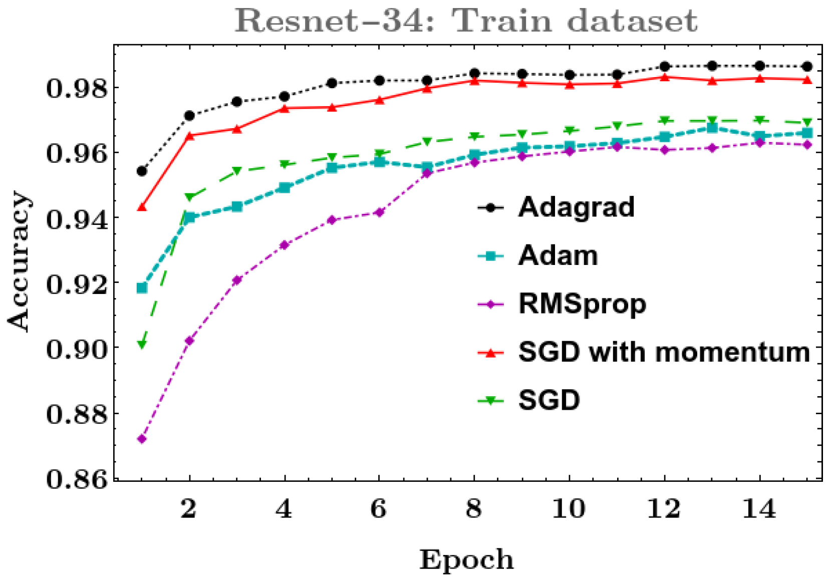
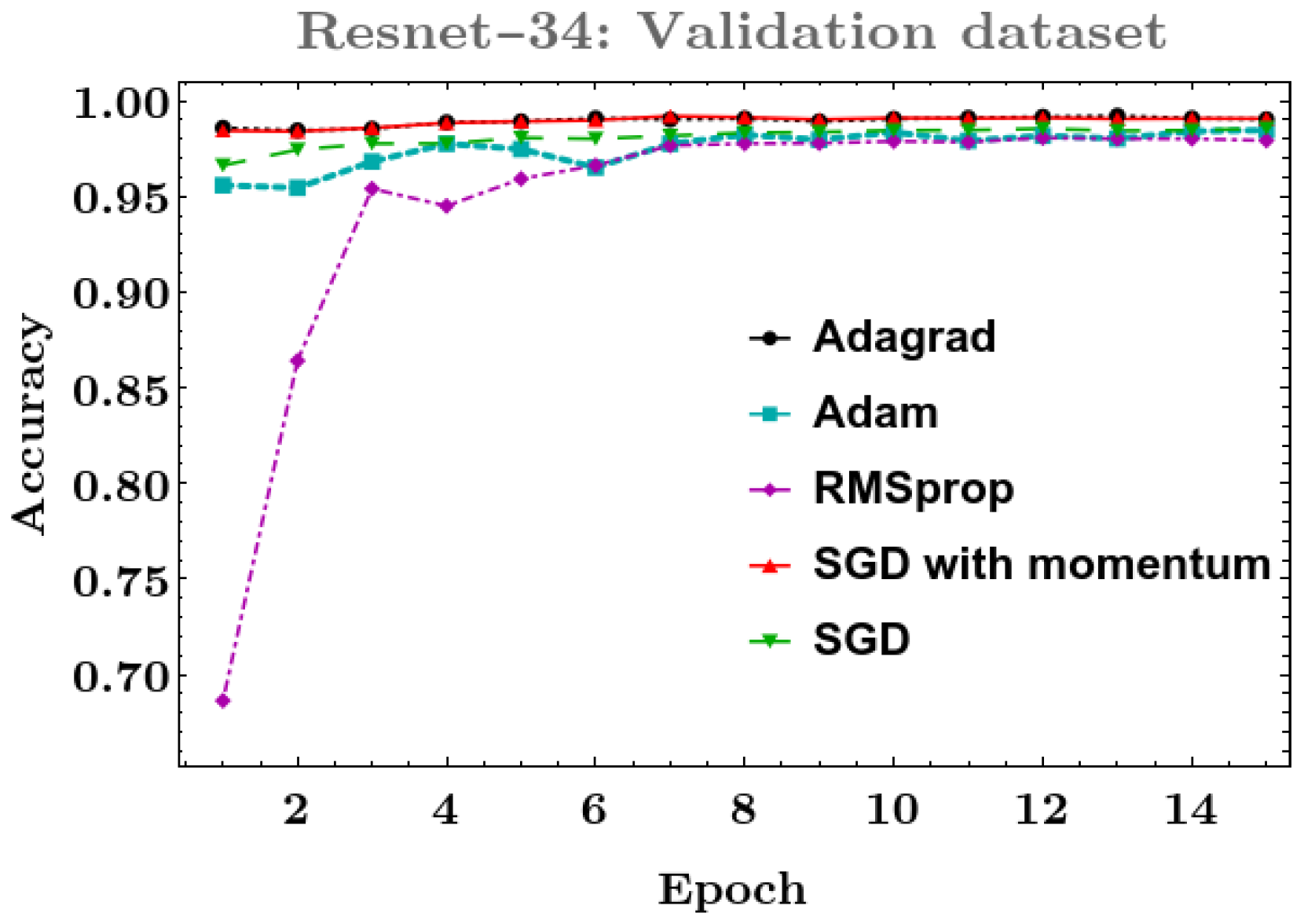
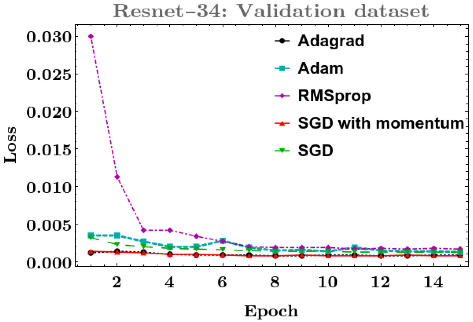
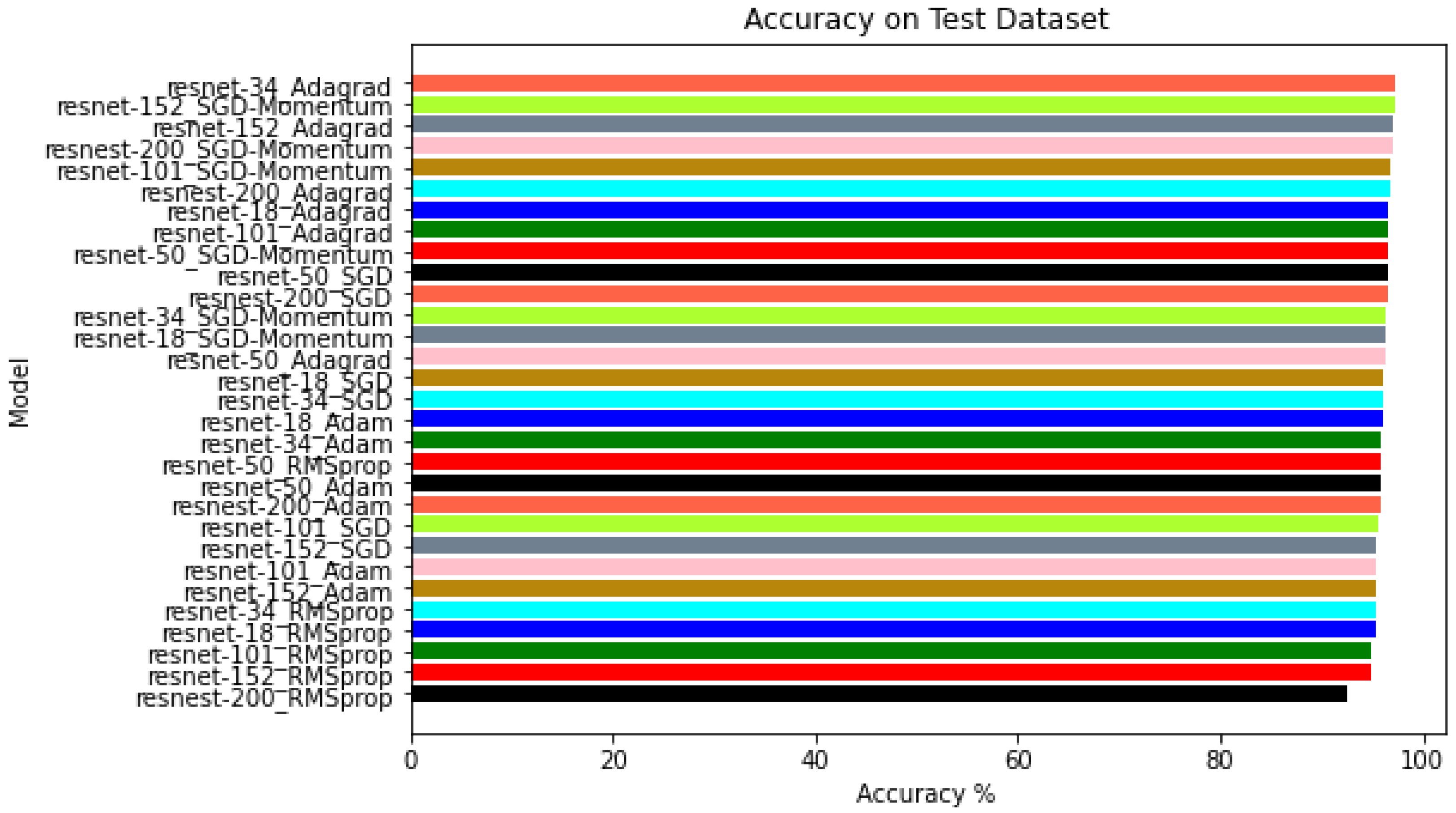
4.1. Phase I: Testing Deep Learning Classification Models with Different Optimizers
- ResNet-18 and ResNet-152: The best performance was obtained with the Adagrad optimizer for both the training and validation datasets.
- ResNet-34, ResNet-50, ResNet-101, and ResNeSt-200: In these models, the best result on the training dataset was obtained with the Adagrad optimizer, and for the validation dataset, SGD with momentum was more robust.


4.2. Phase II: Improving the Dataset, Training the Classification Model for Two Classes, and Extending It to Three Classes
4.2.1. Datasets
4.2.2. Training
4.2.3. Hardware
4.2.4. Results and Analysis
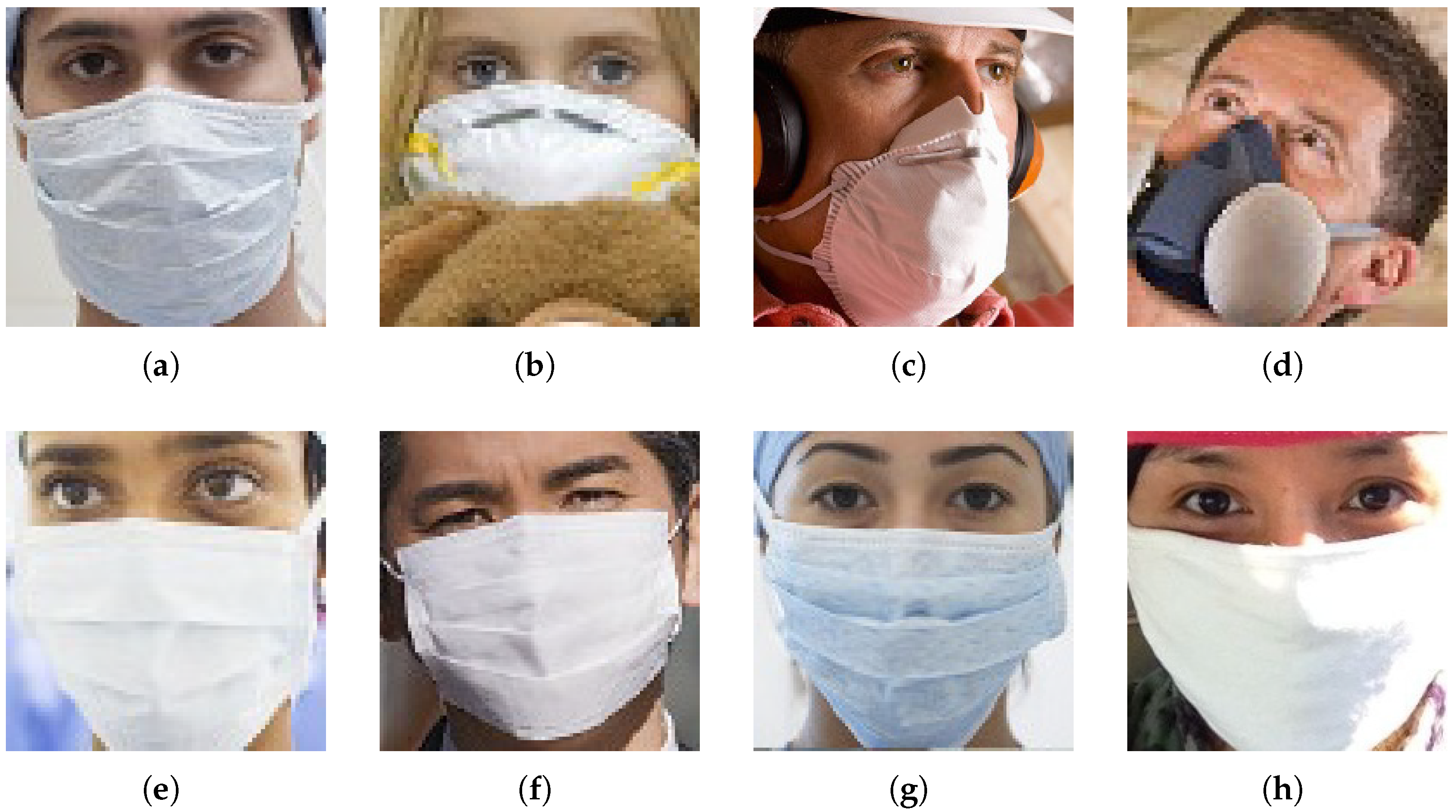
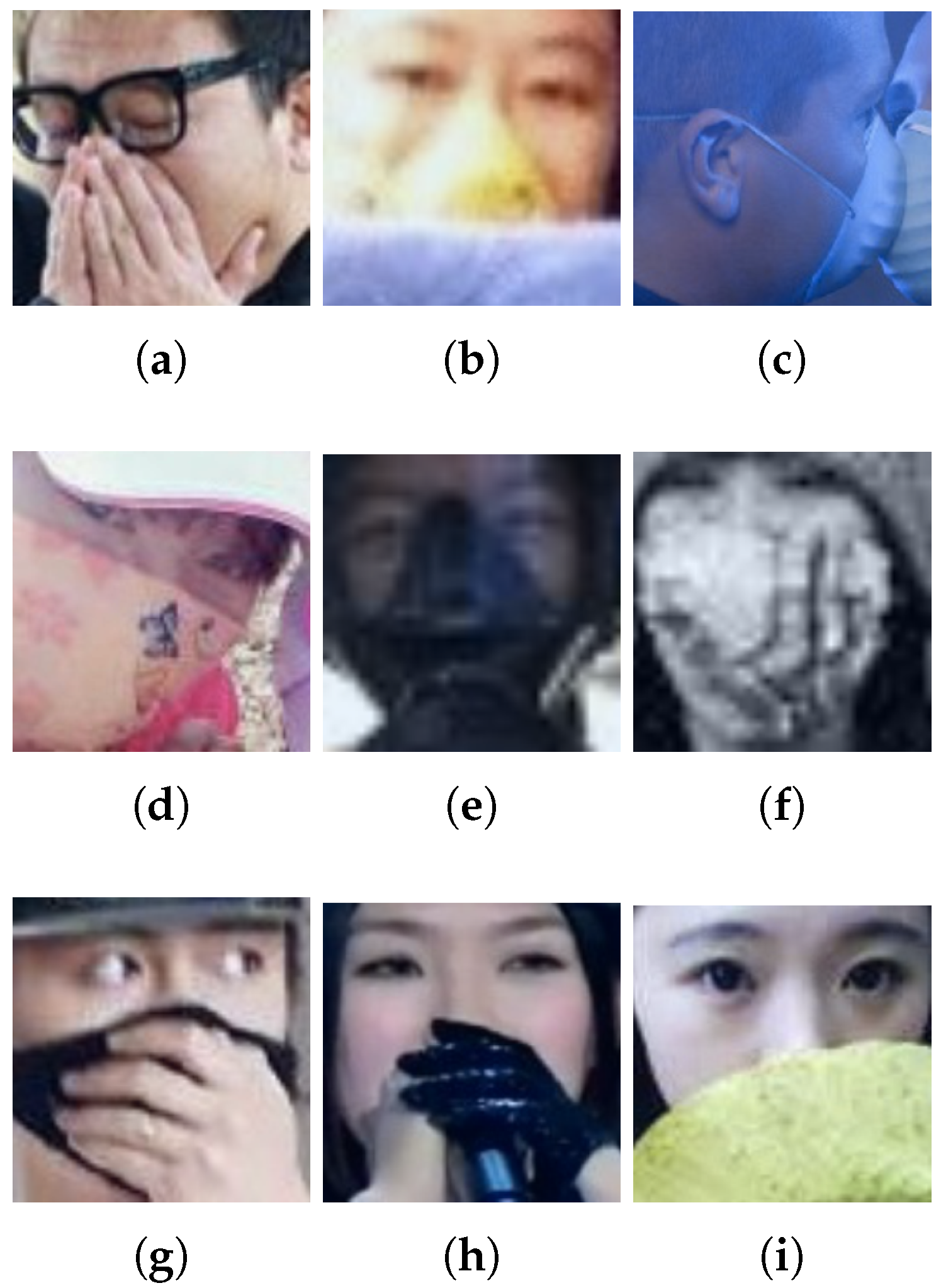
- Compliant images classified as Non-CompliantIn Figure 11, there are three images (Figure 11a,h,i) with the wrong labels, i.e., the true label should be Non-Compliant but they were labeled as Compliant. The last six images were wrongly classified by the model. We can see the model has difficulties with the classification of images of industrial masks (Figure 11b,d) and with profile faces like the image in Figure 11c. We can use Gradient-weighted Class Activation Mapping (Grad-CAM) to visualize the most representative parts of these images for the classification model.Figure 11. Compliant images classified as Non-Compliant.
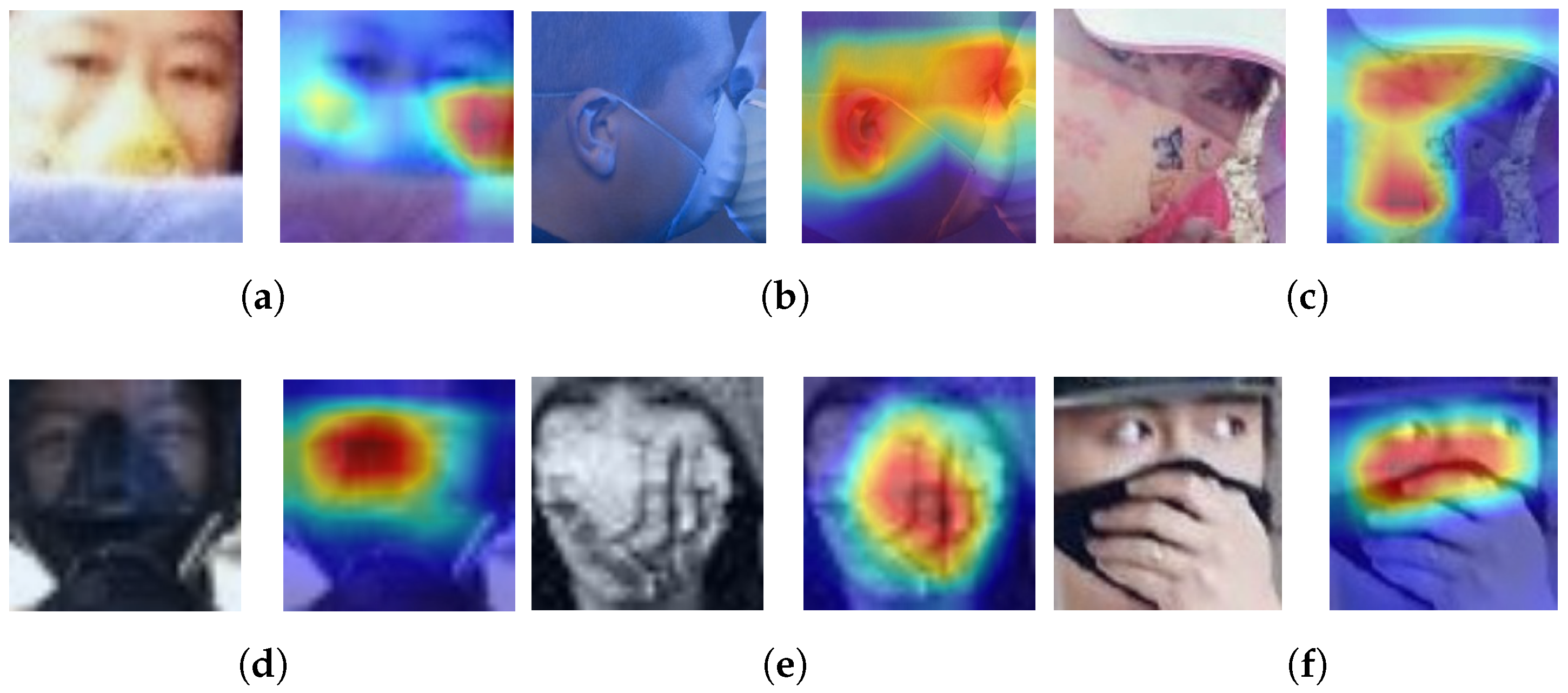
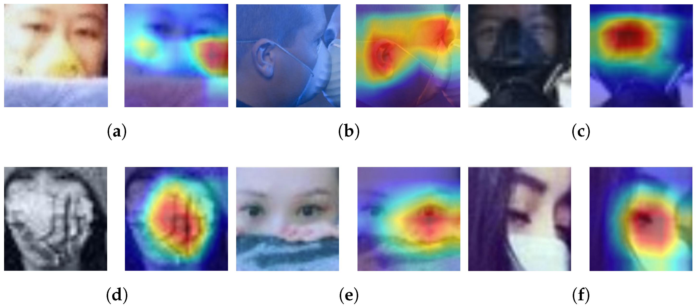
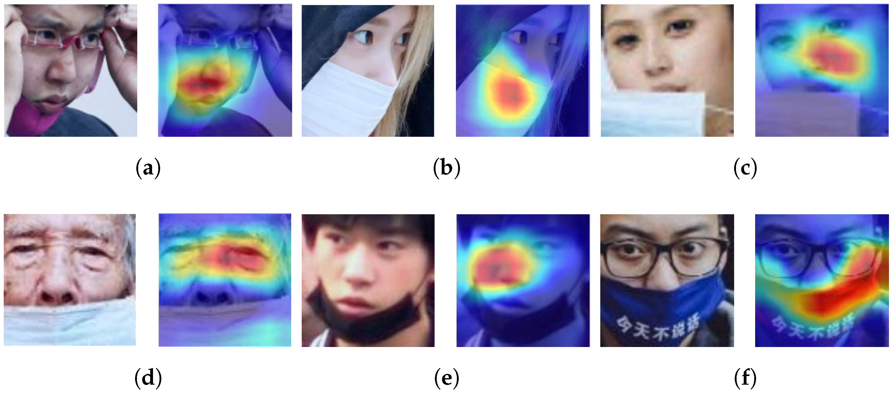
![Applsci 12 06924 g011]() Regarding Grad-CAMs, we find two principal problems. The first is related to the location of the most representative part of the image for the model, when this is not around the nose tip as it should be (images in Figure 12a–d). The second is when the position of the most representative area of the image is correct but the model still cannot make a good classification (images in Figure 12e,f).Figure 12. Compliant images classified as Non-Compliant, analyzed with Grad-CAMs.
Regarding Grad-CAMs, we find two principal problems. The first is related to the location of the most representative part of the image for the model, when this is not around the nose tip as it should be (images in Figure 12a–d). The second is when the position of the most representative area of the image is correct but the model still cannot make a good classification (images in Figure 12e,f).Figure 12. Compliant images classified as Non-Compliant, analyzed with Grad-CAMs.![Applsci 12 06924 g012]()
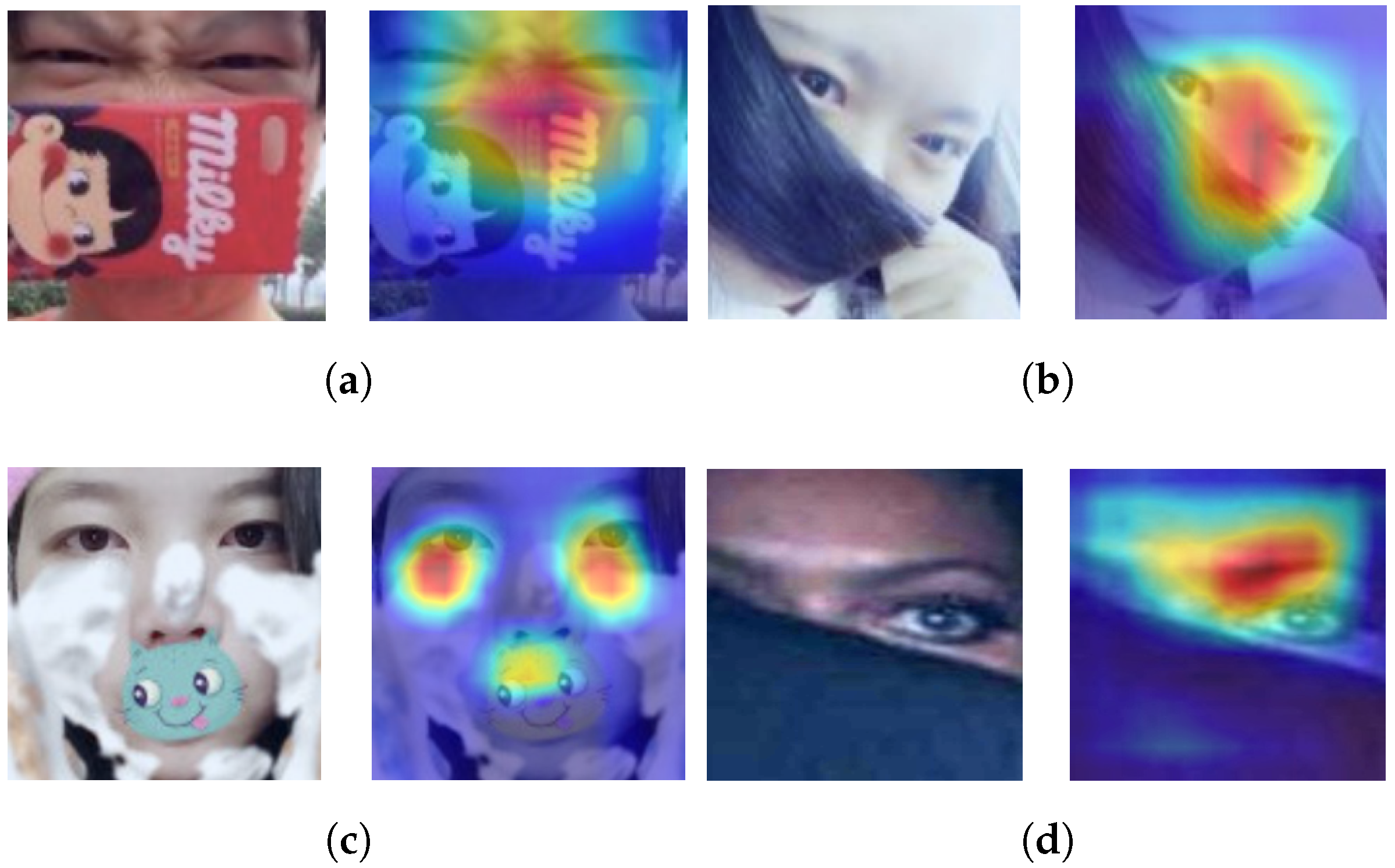
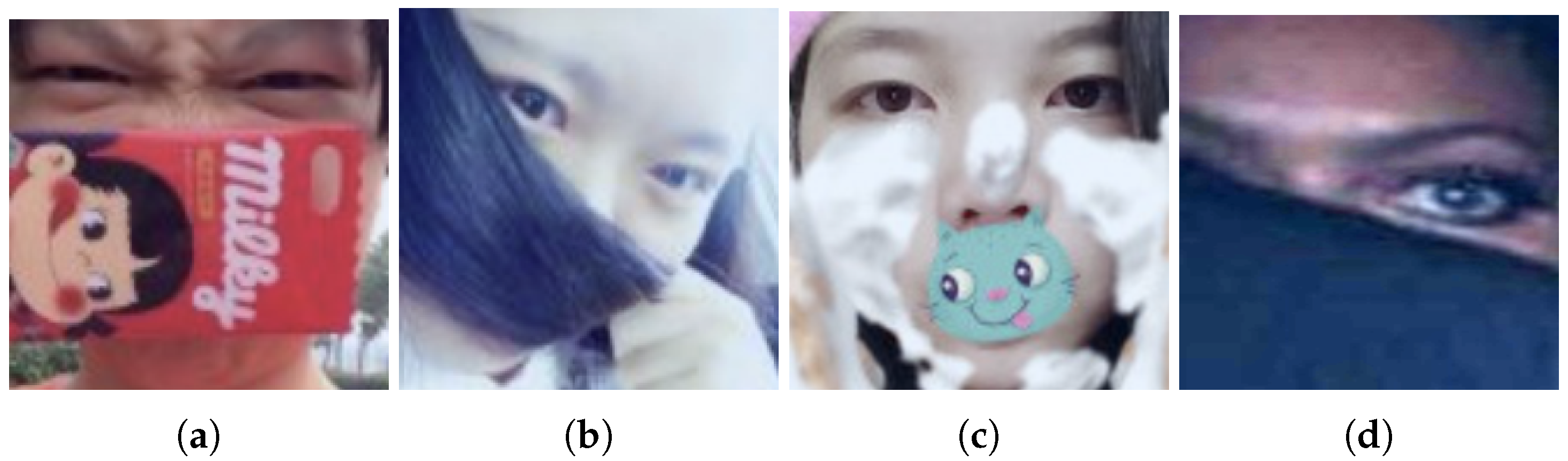
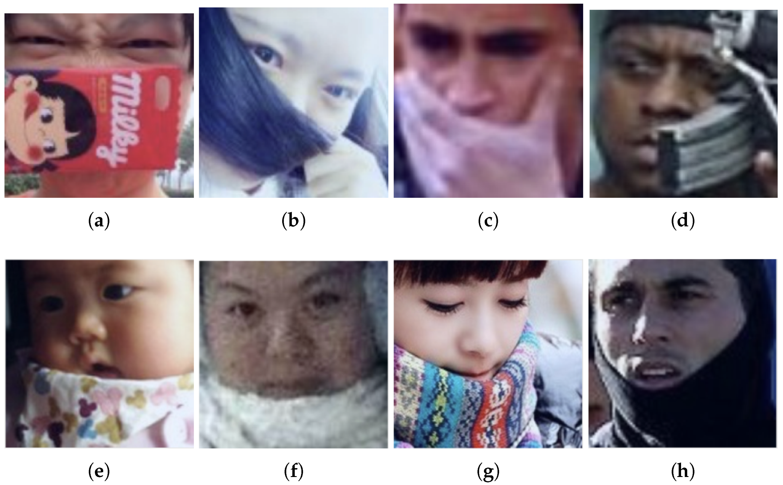
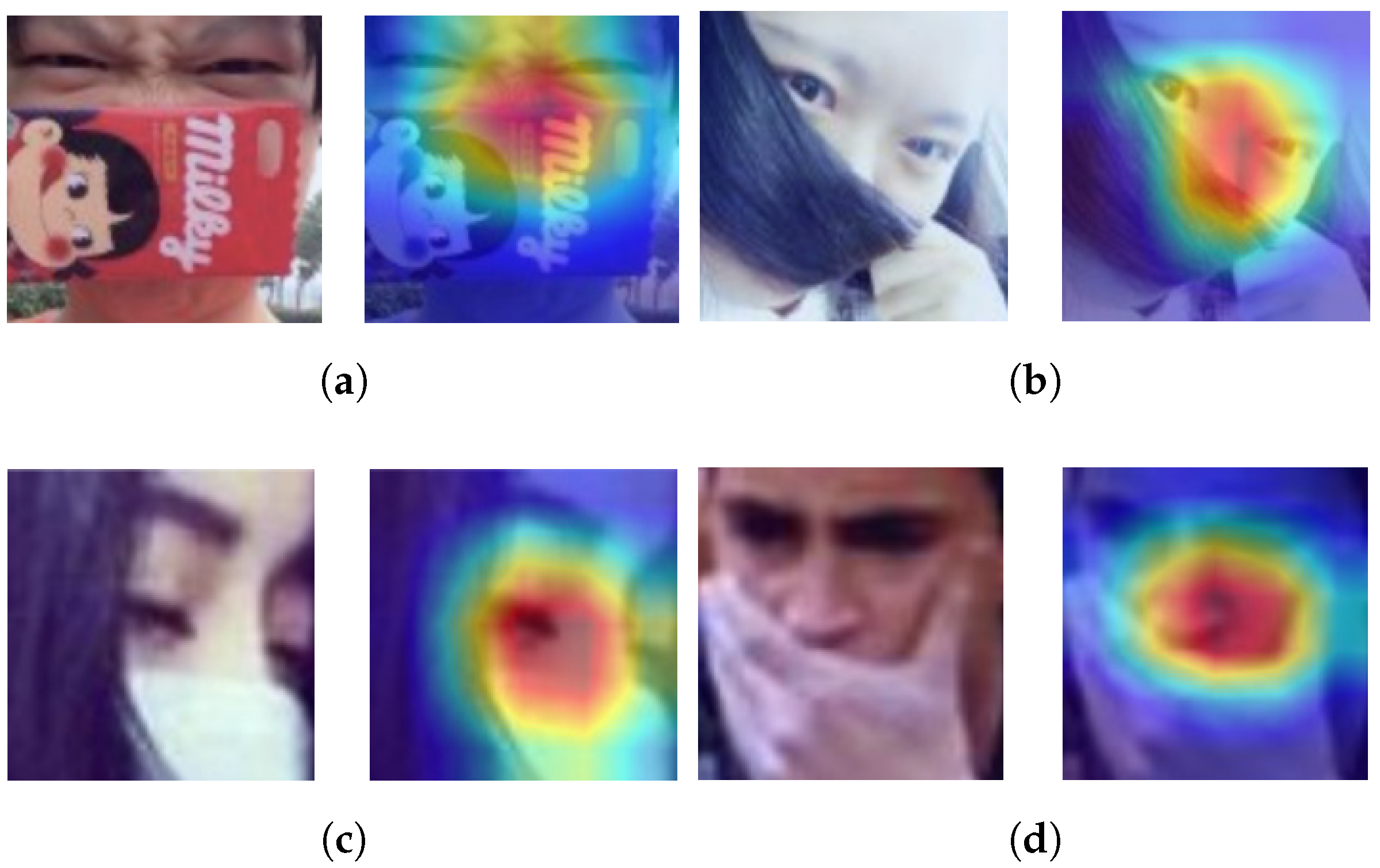
- Non-compliant images classified as CompliantIn Figure 13, the images are wrongly predicted, except the last one which was wrong labeled. The principal cause of the poor performance of the model for these images could be the presence of different objects around the noses. It is probable that the model regards these objects as a COVID-19 mask. The Grad-CAMs presented in Figure 14 help to prove this fact.For the images in Figure 14a,b, we note that the classification model is unable to distinguish between a COVID-19 mask and an object covering the nose. For the last two images (Figure 14c,d), the activation zone is wrong; therefore, these are poor predictions.Figure 13. Non-compliant images classified as compliant.
![Applsci 12 06924 g013]() Figure 14. Non-Compliant images classified as Compliant, analyzed with Grad-CAMs.
Figure 14. Non-Compliant images classified as Compliant, analyzed with Grad-CAMs.![Applsci 12 06924 g014]()


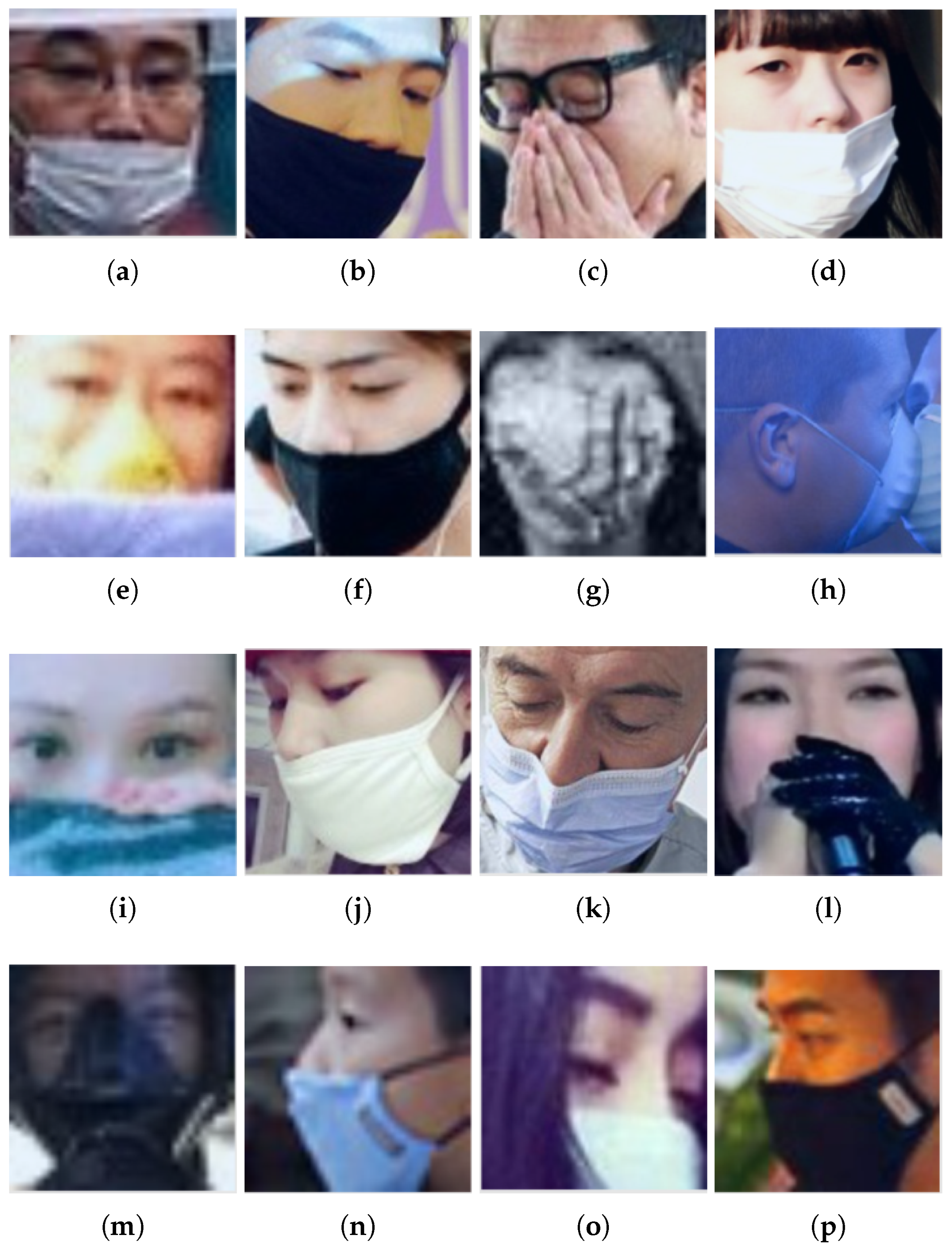
- Compliant images wrongly predictedFigure 17 shows that most of the wrong predictions in this class were related to mistakes in the labeling of the data (images in Figure 17a–d,f,h,j,k,l,n,p), where the prediction was correct but the true label was wrong. In addition, we note that the model had difficulties with images of faces in profile (Figure 17h) and with faces that were very close (Figure 17e,i).There is a way to understand better the reasons for wrong predictions using Grad-CAM. It enables us to visualize which parts of an image were more significant for a model when making a prediction. The Grad-CAM was computed for the wrongly predicted images.Grad-CAMs show a common factor: the most significant part of the image for the model for making the prediction is not the tip of the nose as it should be. In the case of Figure 18b, there is a clear problem related to faces in profile. This could be associated with the lack of profile images in the training dataset, because the proposed model focused on frontal faces. The subjects of the images in Figure 18a–c are wearing nose protection, but it is not a COVID-19 face mask; therefore, a poor prediction was made. Finally, the images in Figure 18e–f are close-ups of the face, and this may have caused the failure in the predicted label.Figure 17. Compliant images wrongly classified. Each image has a predicted label assigned by the ResNet-18 classification model: (a) Incorrect; (b) Incorrect; (c) Non-Compliant; (d) Incorrect; (e) Non-Compliant; (f) Incorrect; (g) Non-Compliant; (h) Non-Compliant; (i) Non-Compliant; (j) Incorrect; (k) Incorrect; (l) Non-Compliant; (m) Non-Compliant; (n) Incorrect; (o) Non-Compliant; (p) Incorrect.Figure 17. Compliant images wrongly classified. Each image has a predicted label assigned by the ResNet-18 classification model: (a) Incorrect; (b) Incorrect; (c) Non-Compliant; (d) Incorrect; (e) Non-Compliant; (f) Incorrect; (g) Non-Compliant; (h) Non-Compliant; (i) Non-Compliant; (j) Incorrect; (k) Incorrect; (l) Non-Compliant; (m) Non-Compliant; (n) Incorrect; (o) Non-Compliant; (p) Incorrect.
![Applsci 12 06924 g017]() Figure 18. Compliant images wrongly predicted, analyzed with Grad-CAMs.
Figure 18. Compliant images wrongly predicted, analyzed with Grad-CAMs.![Applsci 12 06924 g018]()
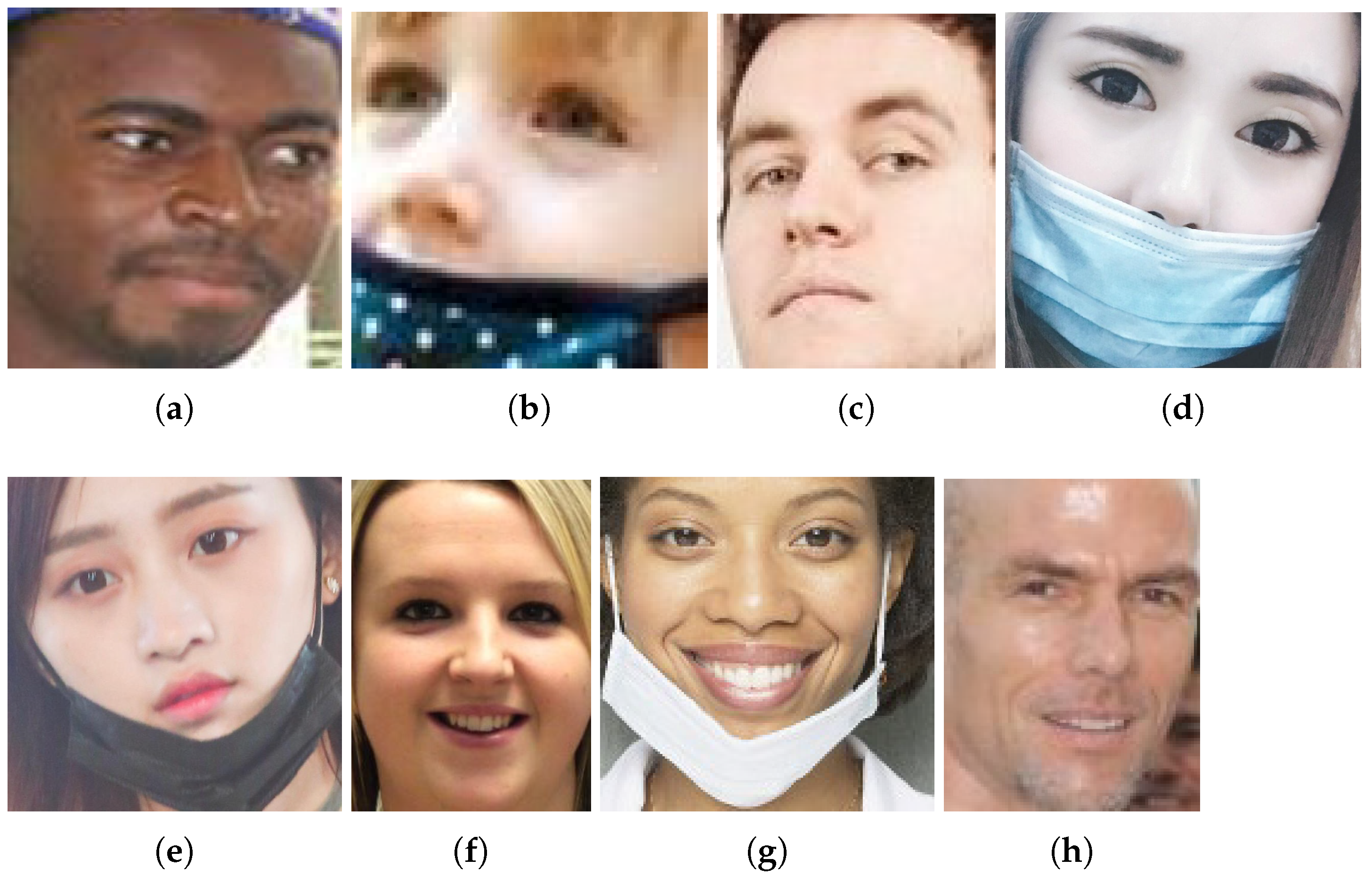
- Non-Compliant images wrongly predictedOne again, there were problems related to the wrong true labels in the images in Figure 19e–h. In addition, there are wrong predictions, especially based on the confusion of COVID-19 face masks with other objects (images in Figure 19a–d). This fact can be seen with the use of Grad-CAMs in Figure 20.Figure 19. Non-Compliant images wrongly classified. Each image has a predicted label assigned by the ResNet-18 classification model: (a) Compliant; (b) Incorrect; (c) Compliant; (d) Incorrect; (e) Incorrect; (f) Incorrect; (g) Incorrect; (h) Incorrect.Figure 19. Non-Compliant images wrongly classified. Each image has a predicted label assigned by the ResNet-18 classification model: (a) Compliant; (b) Incorrect; (c) Compliant; (d) Incorrect; (e) Incorrect; (f) Incorrect; (g) Incorrect; (h) Incorrect.
![Applsci 12 06924 g019]() Figure 20. Non-Compliant images wrongly predicted, analyzed with Grad-CAMs.
Figure 20. Non-Compliant images wrongly predicted, analyzed with Grad-CAMs.![Applsci 12 06924 g020]() According to the Grad-CAM, the more significant parts of the image are located around the nose. Here, we can see objects covering noses that are different from COVID-19 face masks. Therefore, it is probable that the model can sometimes become confused when a nose is covered with some object other than a mask. To solve this problem, it can be helpful to put images with noses covered by other objects and labeled as “Non-Compliant” in the training datasets, to allow the model learn this new feature.
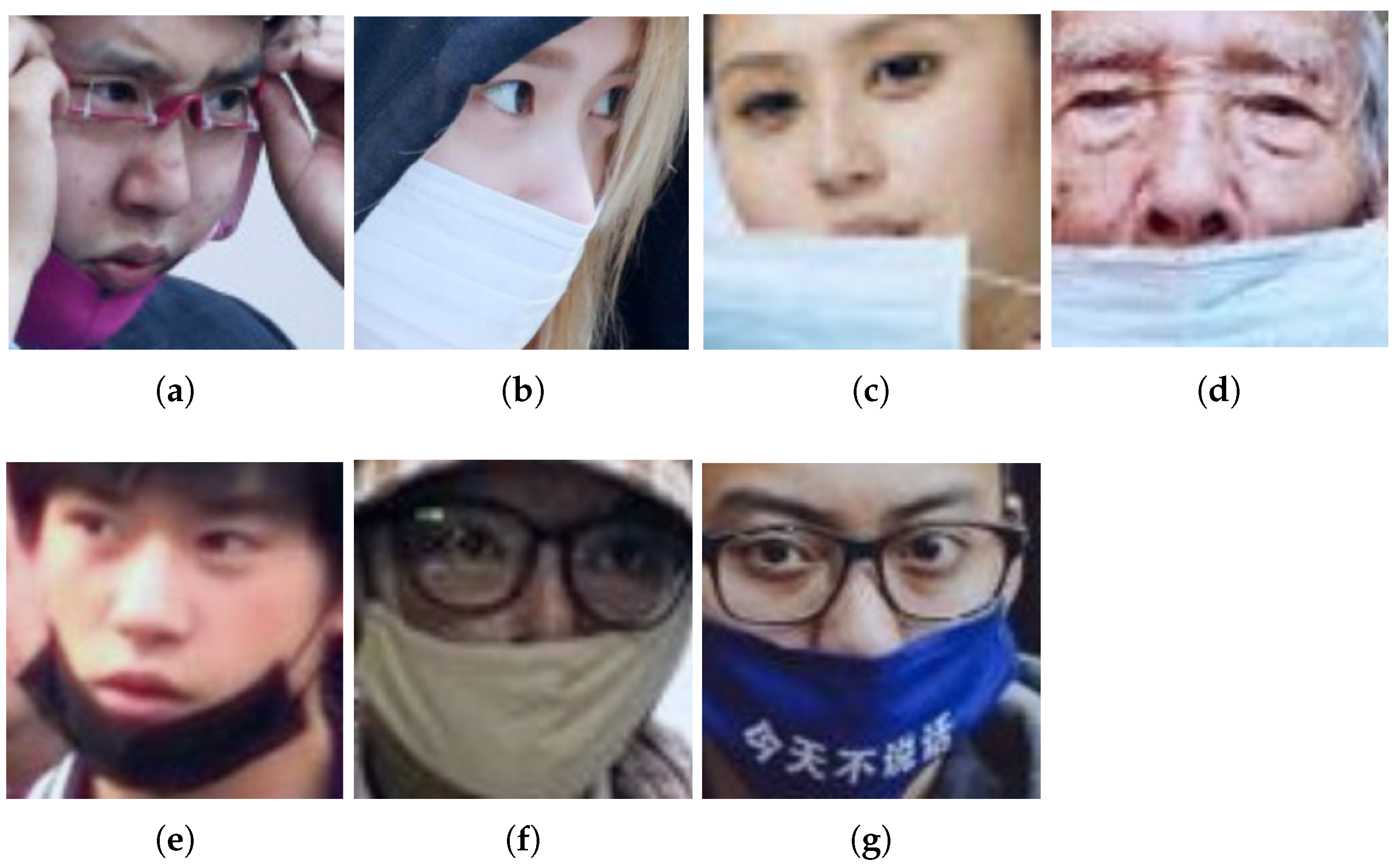
According to the Grad-CAM, the more significant parts of the image are located around the nose. Here, we can see objects covering noses that are different from COVID-19 face masks. Therefore, it is probable that the model can sometimes become confused when a nose is covered with some object other than a mask. To solve this problem, it can be helpful to put images with noses covered by other objects and labeled as “Non-Compliant” in the training datasets, to allow the model learn this new feature. - Incorrect images wrongly predictedThe class “Incorrect” is a particular case, because it can be relative, according to the position of the COVID-19 face mask with respect to the nose. For example, some people consider that the mask is being used incorrectly if it only covers the nasal base. Other people consider the use of the COVID-19 face mask to be incorrect if it does not cover the ridge of the nose entirely. Finally, since many people prefer to put the COVID-19 face mask under the chin to avoid taking it off completely when they want to do not wear it for a short period of time, the position of the COVID-19 face mask under the chin can be considered as “Incorrect”. As we can see, we have different concepts for the Incorrect class, and for this reason, there are some wrong predictions (see Figure 21) related to this fact, which Grad-CAMs can help us to describe.Figure 21. Incorrect images wrongly classified. Each image has a predicted label assigned by the ResNet-18 classification model: (a) Non-Compliant; (b) Compliant; (c) Non-Compliant; (d) Non-Compliant; (e) Non-Compliant; (f) Compliant; (g) Compliant.Figure 21. Incorrect images wrongly classified. Each image has a predicted label assigned by the ResNet-18 classification model: (a) Non-Compliant; (b) Compliant; (c) Non-Compliant; (d) Non-Compliant; (e) Non-Compliant; (f) Compliant; (g) Compliant.
![Applsci 12 06924 g021]() According to Grad-CAMs, the classification model focuses on two principal parts of the image. The first one is around the nasal base, as in the images in Figure 22a,c,e. The second is related to the identification of the COVID-19 face mask (images in Figure 22b,f). In the first case, it may be impossible to classify the image as Incorrect because the model does not focus on the COVID-19 mask, as it is under the chin. As the model identifies the absence of the COVID-19 mask around the nose, the predicted label is Non-Compliant. For the second case, the model only pays attention to the presence of the COVID-19 mask. For this reason, the model cannot identify that the mask is only covering the nasal base, i.e., the mask is used incorrectly, but the model predicts it as Compliant.Figure 22. Incorrect images wrongly predicted, analyzed with Grad-CAMs.
According to Grad-CAMs, the classification model focuses on two principal parts of the image. The first one is around the nasal base, as in the images in Figure 22a,c,e. The second is related to the identification of the COVID-19 face mask (images in Figure 22b,f). In the first case, it may be impossible to classify the image as Incorrect because the model does not focus on the COVID-19 mask, as it is under the chin. As the model identifies the absence of the COVID-19 mask around the nose, the predicted label is Non-Compliant. For the second case, the model only pays attention to the presence of the COVID-19 mask. For this reason, the model cannot identify that the mask is only covering the nasal base, i.e., the mask is used incorrectly, but the model predicts it as Compliant.Figure 22. Incorrect images wrongly predicted, analyzed with Grad-CAMs.![Applsci 12 06924 g022]()


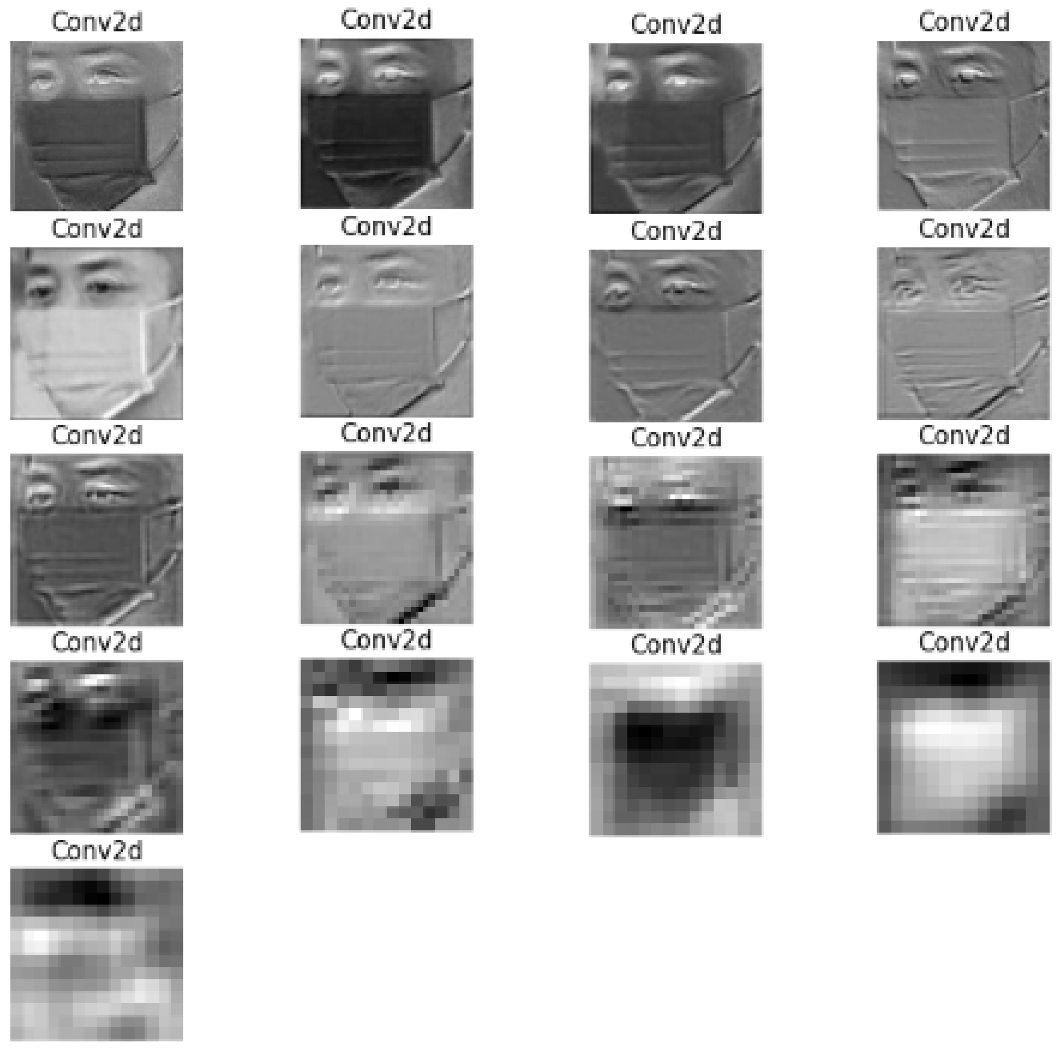
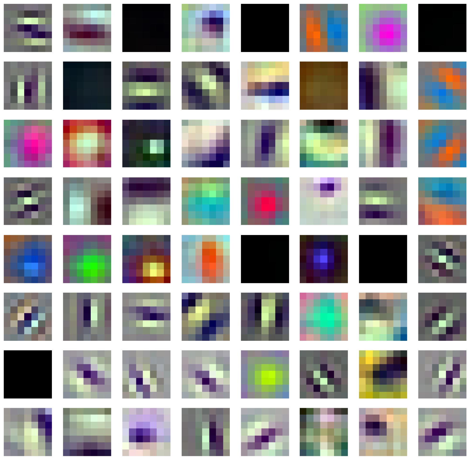
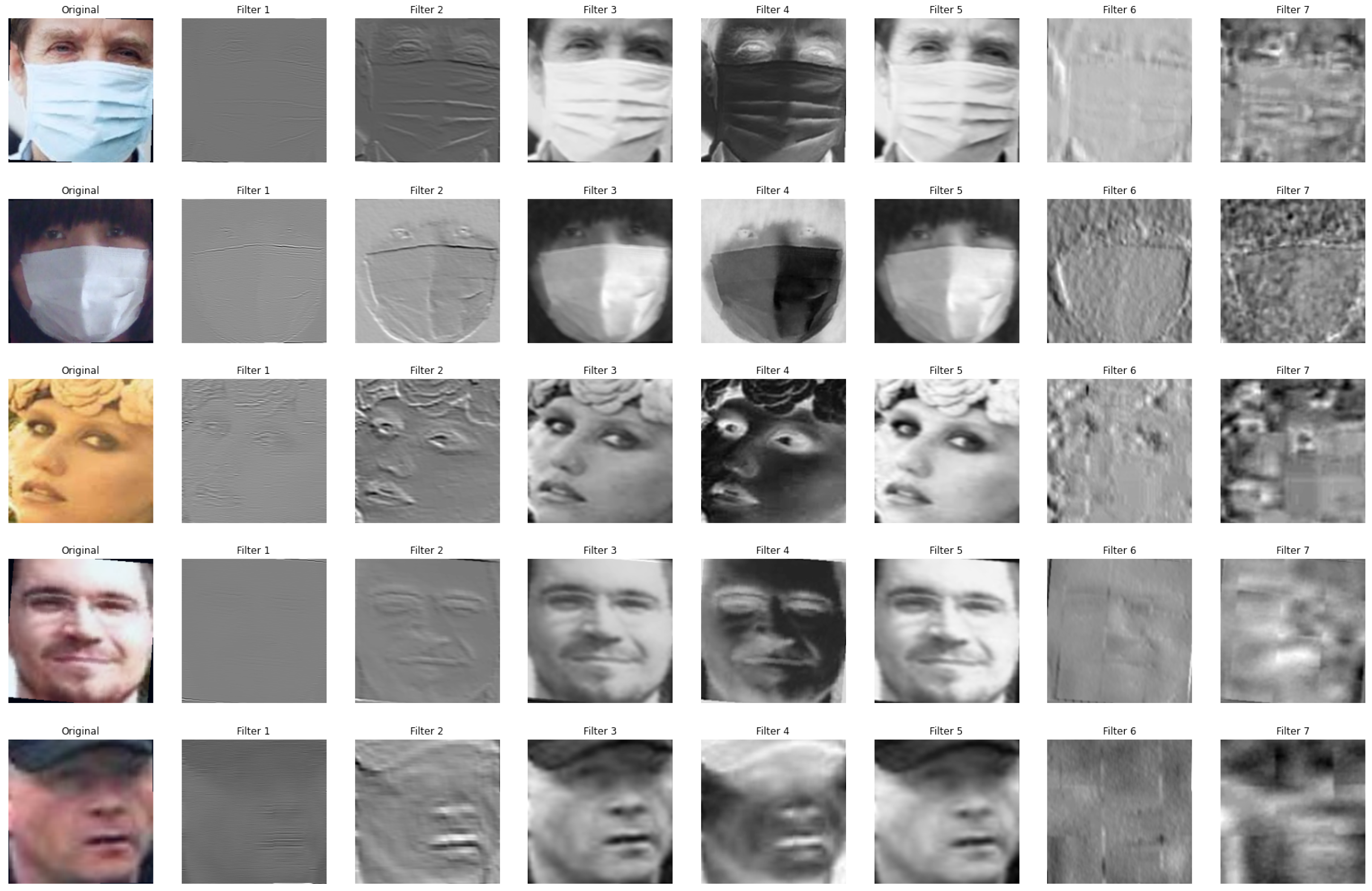
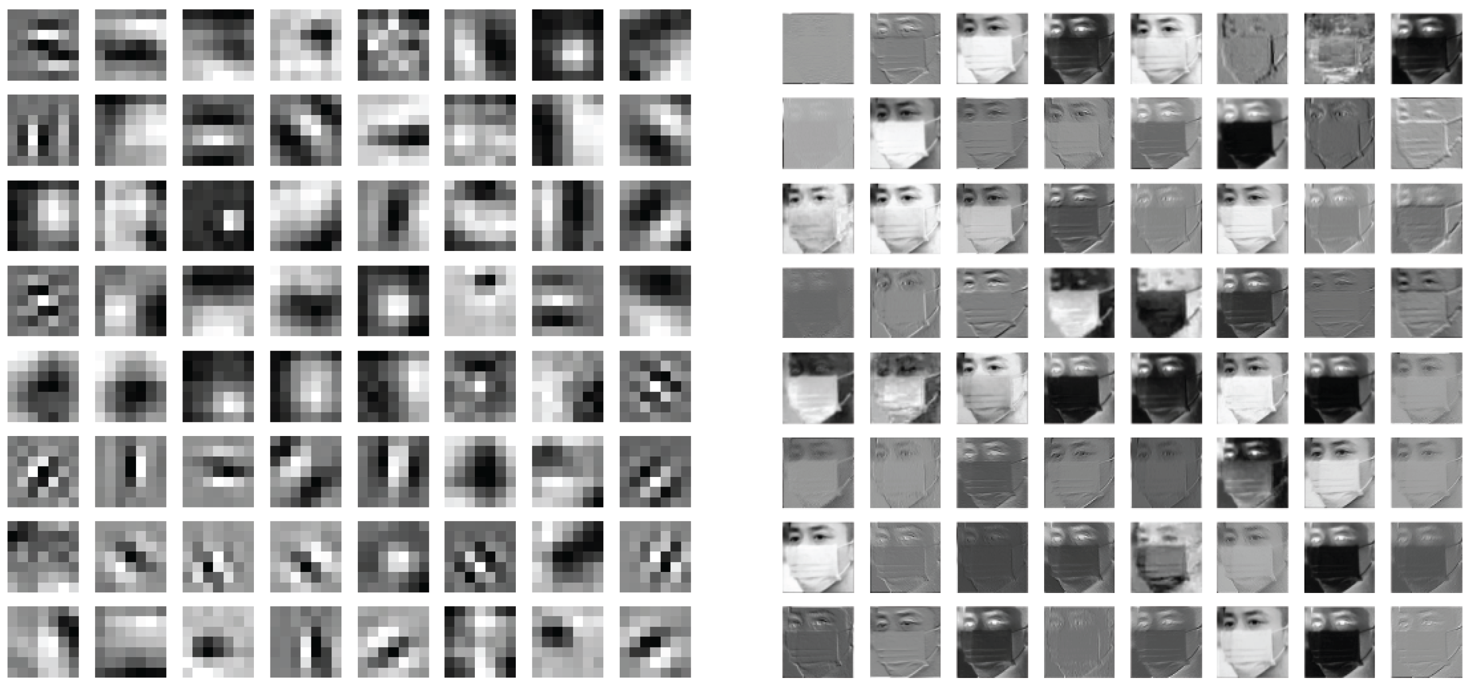
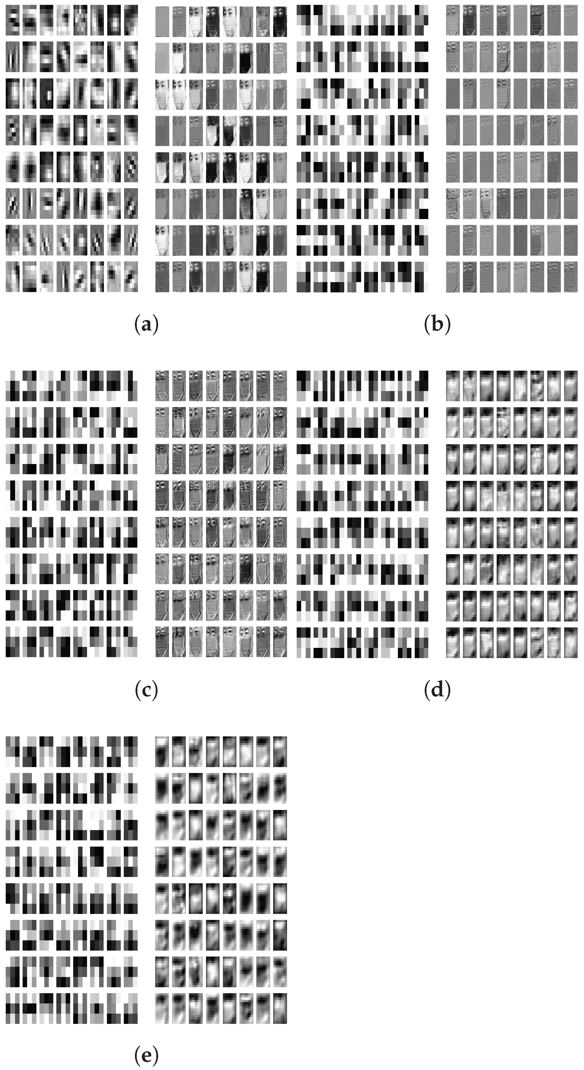
4.3. Visualizing Some Feature Maps and Filters
ResNet-18 Filters
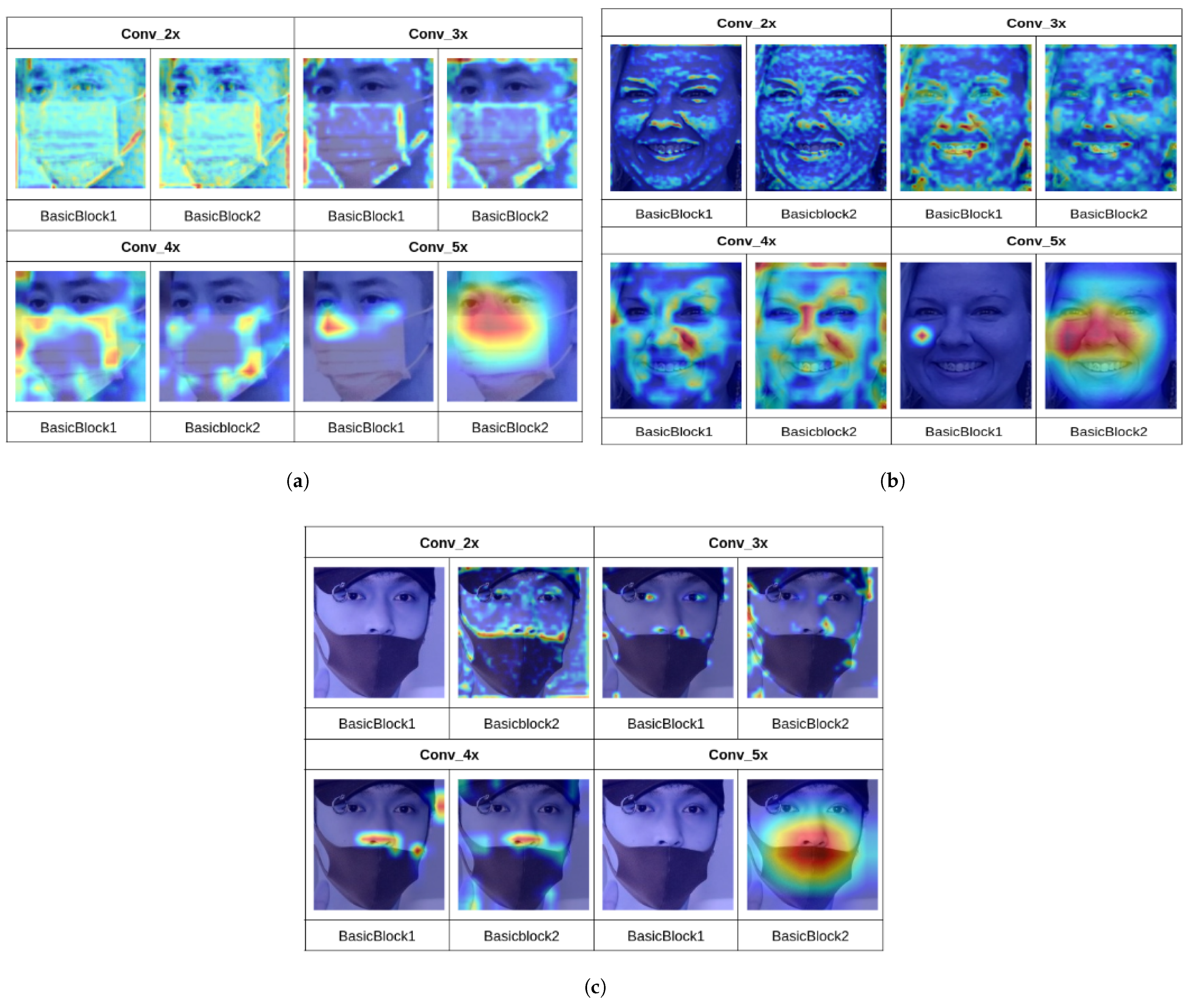
4.4. Grad-CAMs through the Layers
COVID-19 Mask Classification Model with ResNet-18 against Other Approaches
5. Conclusions
5.1. General Conclusions
5.2. Future Work
Author Contributions
Funding
Institutional Review Board Statement
Informed Consent Statement
Data Availability Statement
Conflicts of Interest
References
- Velavan, T.P.; Meyer, C.G. The COVID-19 epidemic. Trop. Med. Int. Health 2020, 25, 278. [Google Scholar] [CrossRef] [PubMed] [Green Version]
- Yuki, K.; Fujiogi, M.; Koutsogiannaki, S. COVID-19 pathophysiology: A review. Clin. Immunol. 2020, 215, 108427. [Google Scholar] [CrossRef]
- Elachola, H.; Ebrahim, S.H.; Gozzer, E. COVID-19: Facemask use prevalence in international airports in Asia, Europe and the Americas, March 2020. Travel Med. Infect. Dis. 2020, 35, 101637. [Google Scholar] [CrossRef]
- Lee, B.Y. How Israel Ended Outdoor Face Mask Mandates with the Help of Covid-19 Vaccines. 2021. Available online: https://www.forbes.com/sites/brucelee/2021/04/20/how-israel-ended-outdoor-face-mask-mandates-with-the-help-of-covid-19-vaccines/?sh=63598b46680e (accessed on 12 April 2022).
- Feng, S.; Shen, C.; Xia, N.; Song, W.; Fan, M.; Cowling, B.J. Rational use of face masks in the COVID-19 pandemic. Lancet Respir. Med. 2020, 8, 434–436. [Google Scholar] [CrossRef]
- Howard, J.; Huang, A.; Li, Z.; Tufekci, Z.; Zdimal, V.; van der Westhuizen, H.M.; von Delft, A.; Price, A.; Fridman, L.; Tang, L.H.; et al. An evidence review of face masks against COVID-19. Proc. Natl. Acad. Sci. USA 2021, 118, e2014564118. [Google Scholar] [CrossRef]
- Eikenberry, S.E.; Mancuso, M.; Iboi, E.; Phan, T.; Eikenberry, K.; Kuang, Y.; Kostelich, E.; Gumel, A.B. To mask or not to mask: Modeling the potential for face mask use by the general public to curtail the COVID-19 pandemic. Infect. Dis. Model. 2020, 5, 293–308. [Google Scholar] [CrossRef]
- Loey, M.; Manogaran, G.; Taha, M.H.N.; Khalifa, N.E.M. Fighting against COVID-19: A novel deep learning model based on YOLO-v2 with ResNet-50 for medical face mask detection. Sustain. Cities Soc. 2021, 65, 102600. [Google Scholar] [CrossRef]
- Castro, R.; Pineda, I.; Lim, W.; Morocho-Cayamcela, M.E. Deep Learning Approaches Based on Transformer Architectures for Image Captioning Tasks. IEEE Access 2022, 10, 33679–33694. [Google Scholar] [CrossRef]
- Castro, R.; Pineda, I.; Morocho-Cayamcela, M.E. Hyperparameter Tuning over an Attention Model for Image Captioning, Proceedings of the Information and Communication Technologies, Ann Arbor, MI, USA, 3–6 June 2021; Salgado Guerrero, J.P., Chicaiza Espinosa, J., Cerrada Lozada, M., Berrezueta-Guzman, S., Eds.; Springer International Publishing: Cham, Switzerland, 2021; pp. 172–183. [Google Scholar]
- Morocho-Cayamcela, M.E.; Lim, W. Pattern recognition of soldier uniforms with dilated convolutions and a modified encoder-decoder neural network architecture. Appl. Artif. Intell. 2021, 35, 476–487. [Google Scholar] [CrossRef]
- Moreno-Revelo, M.Y.; Guachi-Guachi, L.; Gómez-Mendoza, J.B.; Revelo-Fuelagán, J.; Peluffo-Ordóñez, D.H. Enhanced Convolutional-Neural-Network Architecture for Crop Classification. Appl. Sci. 2021, 11, 4292. [Google Scholar] [CrossRef]
- Kirillov, A.; He, K.; Girshick, R.; Rother, C.; Dollár, P. Panoptic Segmentation. In Proceedings of the 2019 IEEE/CVF Conference on Computer Vision and Pattern Recognition (CVPR), Long Beach, CA, USA, 16–20 June 2019; pp. 9396–9405. [Google Scholar] [CrossRef]
- Loey, M.; Manogaran, G.; Taha, M.H.N.; Khalifa, N.E.M. A hybrid deep transfer learning model with machine learning methods for face mask detection in the era of the COVID-19 pandemic. Measurement 2021, 167, 108288. [Google Scholar] [CrossRef] [PubMed]
- Qin, B.; Li, D. Identifying Facemask-Wearing Condition Using Image Super-Resolution with Classification Network to Prevent COVID-19. Sensors 2020, 20, 5236. [Google Scholar] [CrossRef] [PubMed]
- Anaya-Isaza, A.; Mera-Jiménez, L.; Cabrera-Chavarro, J.M.; Guachi-Guachi, L.; Peluffo-Ordóñez, D.; Rios-Patiño, J.I. Comparison of Current Deep Convolutional Neural Networks for the Segmentation of Breast Masses in Mammograms. IEEE Access 2021, 9, 152206–152225. [Google Scholar] [CrossRef]
- Batagelj, B.; Peer, P.; Štruc, V.; Dobrišek, S. How to Correctly Detect Face-Masks for COVID-19 from Visual Information? Appl. Sci. 2021, 11, 2070. [Google Scholar] [CrossRef]
- Loop Hit. Medical Mask Dataset: Humans in the Loop. 2022. Available online: https://humansintheloop.org/medical-mask-dataset (accessed on 1 June 2022).
- Yang, S.; Luo, P.; Loy, C.C.; Tang, X. Wider face: A face detection benchmark. In Proceedings of the IEEE Conference on Computer Vision and Pattern Recognition, Las Vegas, NV, USA, 27–30 June 2016; pp. 5525–5533. [Google Scholar]
- Jain, V.; Learned-Miller, E. Fddb: A Benchmark for Face Detection in Unconstrained Settings; UMass Amherst Technical Report; UMass: Amherts, MA, USA, 2010. [Google Scholar]
- Zhu, X.; Ramanan, D. Face detection, pose estimation, and landmark localization in the wild. In Proceedings of the 2012 IEEE Conference on Computer Vision and Pattern Recognition, Providence, RI, USA, 16–21 June 2012; pp. 2879–2886. [Google Scholar]
- Jain, A.K.; Klare, B.; Park, U. Face recognition: Some challenges in forensics. In Proceedings of the 2011 IEEE International Conference on Automatic Face Gesture Recognition (FG), Santa Barbara, CA, USA, 21–23 March 2011; pp. 726–733. [Google Scholar] [CrossRef] [Green Version]
- Jain, A.K.; Klare, B.; Park, U. Face Matching and Retrieval in Forensics Applications. IEEE MultiMedia 2012, 19, 20. [Google Scholar] [CrossRef]
- Zeng, J.; Zeng, J.; Qiu, X. Deep learning based forensic face verification in videos. In Proceedings of the 2017 International Conference on Progress in Informatics and Computing (PIC), Nanjing, China, 27–29 October 2017; pp. 77–80. [Google Scholar] [CrossRef]
- Ge, S.; Li, J.; Ye, Q.; Luo, Z. Detecting masked faces in the wild with lle-cnns. In Proceedings of the IEEE Conference on Computer Vision and Pattern Recognition, Honolulu, HI, USA, 21–26 July 2017; pp. 2682–2690. [Google Scholar]
- Cabani, A.; Hammoudi, K.; Benhabiles, H.; Melkemi, M. MaskedFace-Net–A dataset of correctly/incorrectly masked face images in the context of COVID-19. Smart Health 2021, 19, 100144. [Google Scholar] [CrossRef]
- Wang, Z.; Wang, G.; Huang, B.; Xiong, Z.; Hong, Q.; Wu, H.; Yi, P.; Jiang, K.; Wang, N.; Pei, Y.; et al. Masked face recognition dataset and application. arXiv 2020, arXiv:2003.09093. [Google Scholar]
- Roy, B.; Nandy, S.; Ghosh, D.; Dutta, D.; Biswas, P.; Das, T. MOXA: A deep learning based unmanned approach for real-time monitoring of people wearing medical masks. Trans. Indian Natl. Acad. Eng. 2020, 5, 509–518. [Google Scholar] [CrossRef]
- Viola, P.; Jones, M. Rapid object detection using a boosted cascade of simple features. In Proceedings of the 2001 IEEE Computer Society Conference on Computer Vision and Pattern Recognition—CVPR, Kauai, HI, USA, 8–14 December 2001; Volume 1, p. I. [Google Scholar]
- Li, H.; Lin, Z.; Shen, X.; Brandt, J.; Hua, G. A convolutional neural network cascade for face detection. In Proceedings of the IEEE Conference on Computer Vision and Pattern Recognition, Boston, MA, USA, 7–12 June 2015; pp. 5325–5334. [Google Scholar]
- Farfade, S.S.; Saberian, M.J.; Li, L.J. Multi-view face detection using deep convolutional neural networks. In Proceedings of the 5th ACM on International Conference on Multimedia Retrieval, Shanghai, China, 23–26 June 2015; pp. 643–650. [Google Scholar]
- Sun, X.; Wu, P.; Hoi, S.C. Face detection using deep learning: An improved faster RCNN approach. Neurocomputing 2018, 299, 42–50. [Google Scholar] [CrossRef] [Green Version]
- Zhang, S.; Chi, C.; Lei, Z.; Li, S.Z. Refineface: Refinement neural network for high performance face detection. IEEE Trans. Pattern Anal. Mach. Intell. 2020, 43, 4008–4020. [Google Scholar] [CrossRef]
- Gao, J.; Yang, T. Face detection algorithm based on improved TinyYOLOv3 and attention mechanism. Comput. Commun. 2022, 181, 329–337. [Google Scholar] [CrossRef]
- Li, Y. Face Detection Algorithm Based on Double-Channel CNN with Occlusion Perceptron. Comput. Intell. Neurosci. 2022, 2022, 3705581. [Google Scholar] [CrossRef] [PubMed]
- Wu, P.; Li, H.; Zeng, N.; Li, F. FMD-Yolo: An efficient face mask detection method for COVID-19 prevention and control in public. Image Vis. Comput. 2022, 117, 104341. [Google Scholar] [CrossRef] [PubMed]
- Zhang, J.; Han, F.; Chun, Y.; Chen, W. A novel detection framework about conditions of wearing face mask for helping control the spread of covid-19. IEEE Access 2021, 9, 42975–42984. [Google Scholar] [CrossRef]
- Lin, H.; Tse, R.; Tang, S.K.; Chen, Y.; Ke, W.; Pau, G. Near-realtime face mask wearing recognition based on deep learning. In Proceedings of the 2021 IEEE 18th Annual Consumer Communications & Networking Conference (CCNC), Las Vegas, NV, USA, 9–12 January 2021; pp. 1–7. [Google Scholar]
- Xiong, Y.; Zhu, K.; Lin, D.; Tang, X. Recognize complex events from static images by fusing deep channels. In Proceedings of the IEEE Conference on Computer Vision and Pattern Recognition, Boston, MA, USA, 7–12 June 2015; pp. 1600–1609. [Google Scholar]
- Deng, J.; Guo, J.; Zhou, Y.; Yu, J.; Kotsia, I.; Zafeiriou, S. Retinaface: Single-stage dense face localisation in the wild. arXiv 2019, arXiv:1905.00641. [Google Scholar]
- Krizhevsky, A.; Sutskever, I.; Hinton, G.E. Imagenet classification with deep convolutional neural networks. Adv. Neural Inf. Process. Syst. 2012, 25, 1097–1105. [Google Scholar] [CrossRef]
- He, K.; Zhang, X.; Ren, S.; Sun, J. Deep residual learning for image recognition. In Proceedings of the IEEE Conference on Computer Vision and Pattern Recognition, Las Vegas, NV, USA, 27–30 June 2016; pp. 770–778. [Google Scholar]
- Zhang, H.; Wu, C.; Zhang, Z.; Zhu, Y.; Lin, H.; Zhang, Z.; Sun, Y.; He, T.; Mueller, J.; Manmatha, R.; et al. Resnest: Split-attention networks. arXiv 2020, arXiv:2004.08955. [Google Scholar]
- Morocho-Cayamcela, M.E.; Lee, H.; Lim, W. Machine Learning to Improve Multi-Hop Searching and Extended Wireless Reachability in V2X. IEEE Commun. Lett. 2020, 24, 1477–1481. [Google Scholar] [CrossRef] [Green Version]
- Duchi, J.; Hazan, E.; Singer, Y. Adaptive subgradient methods for online learning and stochastic optimization. J. Mach. Learn. Res. 2011, 12, 2121–2159. [Google Scholar]
- Kingma, D.P.; Ba, J. Adam: A method for stochastic optimization. arXiv 2014, arXiv:1412.6980. [Google Scholar]
- Robbins, H.; Monro, S. A stochastic approximation method. Ann. Math. Stat. 1951, 22, 400–407. [Google Scholar] [CrossRef]
- Ruder, S. An overview of gradient descent optimization algorithms. arXiv 2016, arXiv:1609.04747. [Google Scholar]
- Oumina, A.; El Makhfi, N.; Hamdi, M. Control the covid-19 pandemic: Face mask detection using transfer learning. In Proceedings of the 2020 IEEE 2nd International Conference on Electronics, Control, Optimization and Computer Science (ICECOCS), Kenitra, Morocco, 2–3 December 2020; pp. 1–5. [Google Scholar]


| Donor Dataset | Purpose | Images | Faces | Labels | ||
|---|---|---|---|---|---|---|
| With Mask | Without Mask | |||||
| Correct | Incorrect | |||||
| MAFA | Training | 25,876 | 29,452 | 24,603 | 1204 | 3645 |
| Testing | 4935 | 7342 | 4929 | 324 | 2089 | |
| WIDER FACE | Training | 8906 | 20,932 | 0 | 0 | 20,932 |
| Testing | 2217 | 5346 | 0 | 0 | 5346 | |
| FMLD | Training | 34,782 | 50,384 | 24,603 | 1204 | 24,577 |
| Testing | 7152 | 12,688 | 4929 | 324 | 7435 | |
| Totals | 41,934 | 63,072 | 29,532 | 1528 | 32,012 | |
| Dataset | Classes | |
|---|---|---|
| Compliant | Non-Compliant | |
| Training | 7028 | 17,525 |
| Validation | 1757 | 4382 |
| Test | 4795 | 137,50 |
| Total | 13,580 | 35,657 |
| Accuracy % | |||||
|---|---|---|---|---|---|
| Model | SGD | RMSprop | Adam | SGD with Momentum | Adagrad |
| ResNeSt-200 | 96.44 | 92.41 | 95.79 | 97.01 | 96.78 |
| ResNet-18 | 96.06 | 95.24 | 95.95 | 96.35 | 96.64 |
| ResNet-34 | 96.06 | 95.28 | 95.86 | 96.4 | 97.24 |
| ResNet-50 | 96.54 | 95.82 | 95.82 | 96.59 | 96.21 |
| ResNet-101 | 95.64 | 94.95 | 95.29 | 96.8 | 96.63 |
| ResNet-152 | 95.33 | 94.92 | 95.29 | 97.21 | 97.08 |
| Dataset | Classes | |
|---|---|---|
| Compliant | Non-Compliant | |
| Training | 20,937 | 20,937 |
| Validation | 1231 | 1231 |
| Test | 2463 | 2463 |
| Total | 24,631 | 24,631 |
| Dataset | Classes | ||
|---|---|---|---|
| Compliant | Incorrect | Non-Compliant | |
| Training | 20,937 | 935 | 20,937 |
| Validation | 1231 | 55 | 1231 |
| Test | 2463 | 109 | 2463 |
| Total | 24,631 | 1099 | 24,631 |
| Precision | Recall | F1-Score | Images | |
|---|---|---|---|---|
| Compliant | 1.00 | 0.99 | 1.00 | 2463 |
| Non-Compliant | 0.99 | 1.00 | 1.00 | 2463 |
| Precision | Recall | F1-Score | Images | |
|---|---|---|---|---|
| Compliant | 1.00 | 0.99 | 0.99 | 2463 |
| Incorrect | 0.86 | 0.90 | 0.88 | 109 |
| Non-Compliant | 0.99 | 1.00 | 0.99 | 2463 |
| Models | Recall | Precision |
|---|---|---|
| MobileNetV2 and SVM | 94.84% | 95.08% |
| VGG19 and KNN | 90.09% | 91.3% |
| ResNet-18 | 98% | 98% |
Publisher’s Note: MDPI stays neutral with regard to jurisdictional claims in published maps and institutional affiliations. |
© 2022 by the authors. Licensee MDPI, Basel, Switzerland. This article is an open access article distributed under the terms and conditions of the Creative Commons Attribution (CC BY) license (https://creativecommons.org/licenses/by/4.0/).
Share and Cite
Crespo, F.; Crespo, A.; Sierra-Martínez, L.M.; Peluffo-Ordóñez, D.H.; Morocho-Cayamcela, M.E. A Computer Vision Model to Identify the Incorrect Use of Face Masks for COVID-19 Awareness. Appl. Sci. 2022, 12, 6924. https://doi.org/10.3390/app12146924
Crespo F, Crespo A, Sierra-Martínez LM, Peluffo-Ordóñez DH, Morocho-Cayamcela ME. A Computer Vision Model to Identify the Incorrect Use of Face Masks for COVID-19 Awareness. Applied Sciences. 2022; 12(14):6924. https://doi.org/10.3390/app12146924
Chicago/Turabian StyleCrespo, Fabricio, Anthony Crespo, Luz Marina Sierra-Martínez, Diego Hernán Peluffo-Ordóñez, and Manuel Eugenio Morocho-Cayamcela. 2022. "A Computer Vision Model to Identify the Incorrect Use of Face Masks for COVID-19 Awareness" Applied Sciences 12, no. 14: 6924. https://doi.org/10.3390/app12146924
APA StyleCrespo, F., Crespo, A., Sierra-Martínez, L. M., Peluffo-Ordóñez, D. H., & Morocho-Cayamcela, M. E. (2022). A Computer Vision Model to Identify the Incorrect Use of Face Masks for COVID-19 Awareness. Applied Sciences, 12(14), 6924. https://doi.org/10.3390/app12146924