
A Lightweight Multi-Source Fast Android Malware Detection Model


Abstract
:1. Introduction
1.1. Background
1.2. Motivation
1.3. Our Works
- We propose a multi-source approach for Android malware detection which uses multiple files in an Android application package. It extracts relevant features contained in the files from multiple dimensions, such as information in the file headers and the power spectral density of the structural entropy of the executable file, which makes the extraction of features more comprehensive.
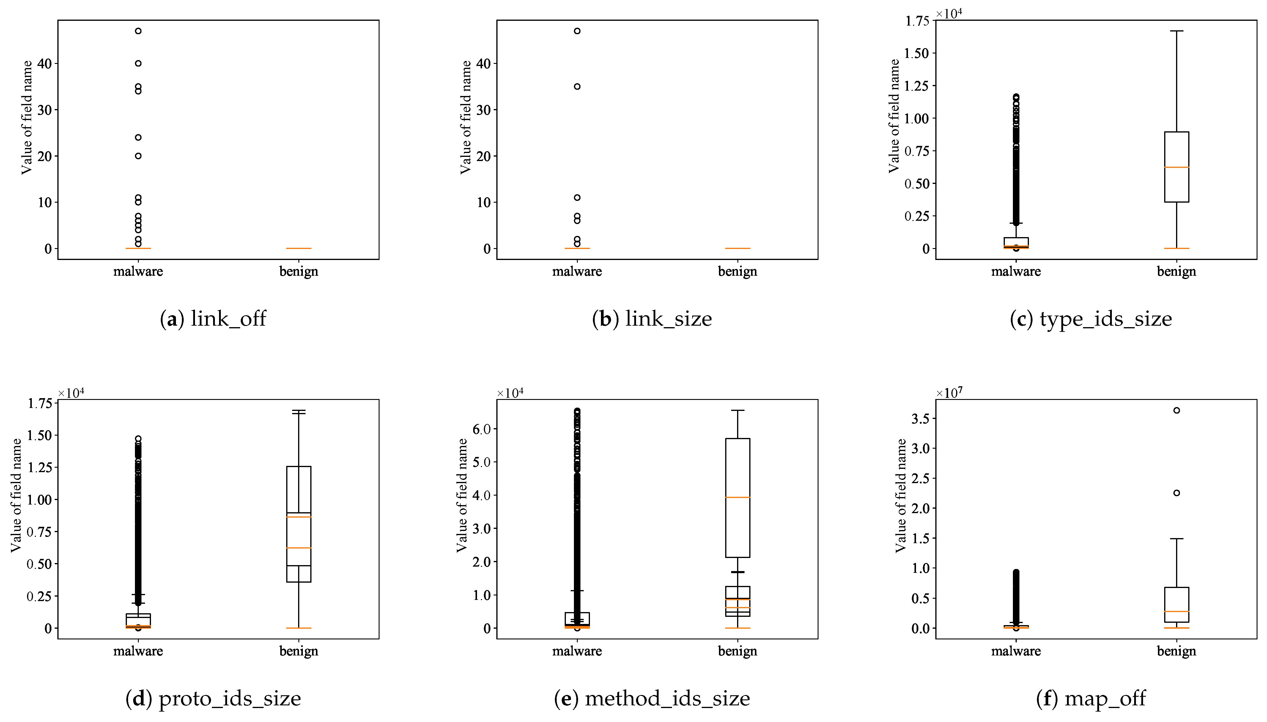
- We studied the information in each field of the header of DEX files and found some key features in the DEX file header that can be used for malware detection. Therefore, a DEX header parser is proposed to extract key features from the DEX file header.
- We propose an adaptive shrinkage convolutional neural network, which can dynamically adjust the convolutional kernel weights and activation function thresholds through an attention mechanism, making the convolutional network with denoising ability while improving the expressiveness of the neural network model.
- We propose a new adaptive soft voting method, which can dynamically change the weight of each base model during the training process, overcoming the noise generated by the traditional soft voting due to the large performance gap and jitter of the base models, while significantly improving the performance of soft voting.
2. Related Work
2.1. Static Analysis
2.2. Dynamic Analysis
2.3. Hybrid Analysis
3. A Lightweight Multi-Source Fast Android Malware Detection Model
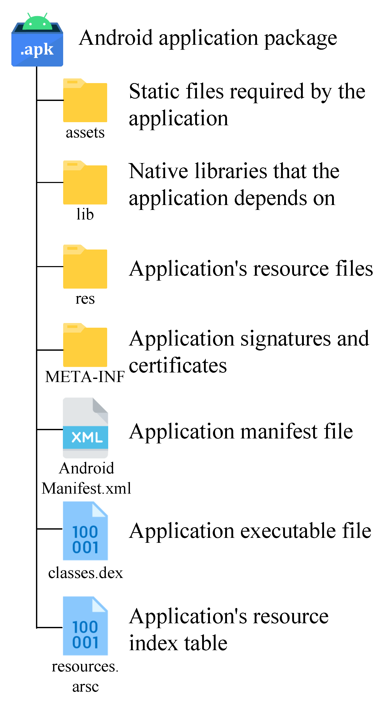
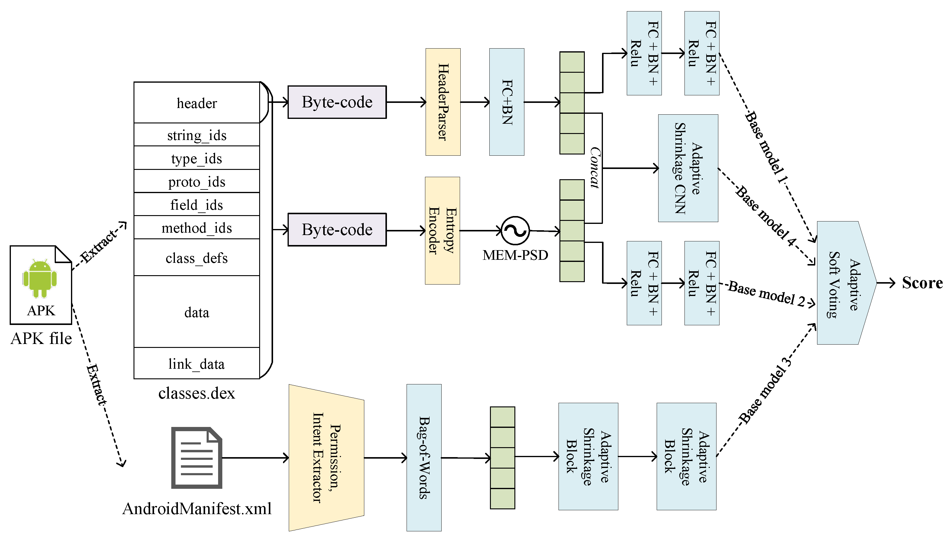
3.1. Android Application Structure and Its Feature Selection and Feature Extraction Scheme
3.2. Ensemble Model and Base Models
- Base model 1: Abbreviated as . It extract and parse the header information of the classes.dex file, encode it as header features, and use the multilayer perceptron for prediction;
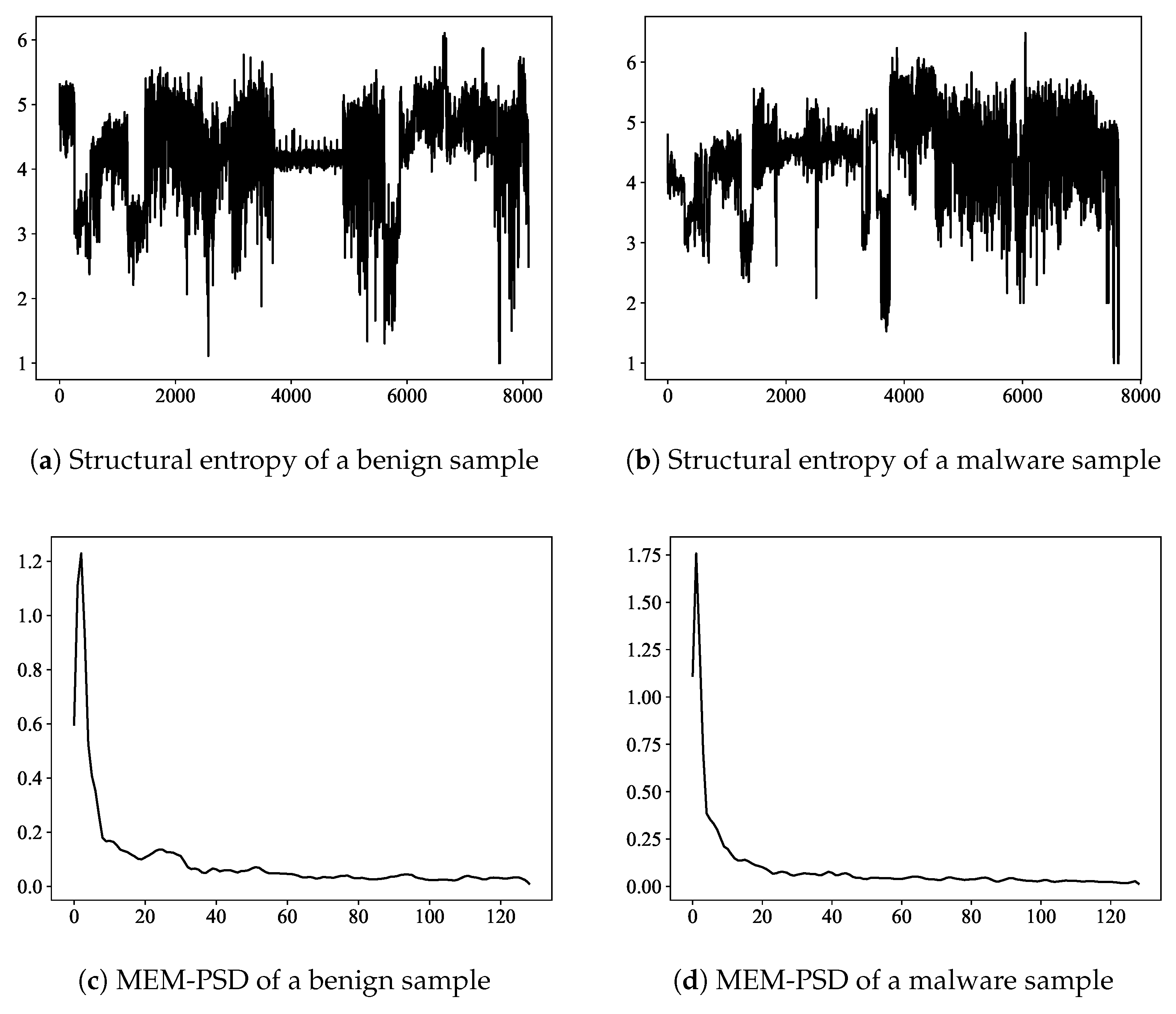
- Base model 2: Abbreviated as . It calculate the entropy of the classses.dex file, extract the power spectral density of the entropy signal as features by the maximum entropy method, and use the multilayer perceptron for prediction as well;
- Base model 3: Abbreviated as . perform the prediction on the AndroidManifest.xml file is decoded and parsed. Permission and intent keywords are extracted and encoded as features by bag-of-words model. Since the dimensionality is too high, we use adaptive shrinkage convolutional neural network for dimensionality reduction and then prediction by multilayer perceptron;
- Base model 4: Abbreviated as . Since theoretically using more base models for ensemble learning will give better results. To improve the ensemble learning, we additionally added a base model that concatenate the features extracted from the DEX file header and the permission and intent features and uses an adaptive shrinkage convolutional neural network and a multilayer perceptron for prediction.
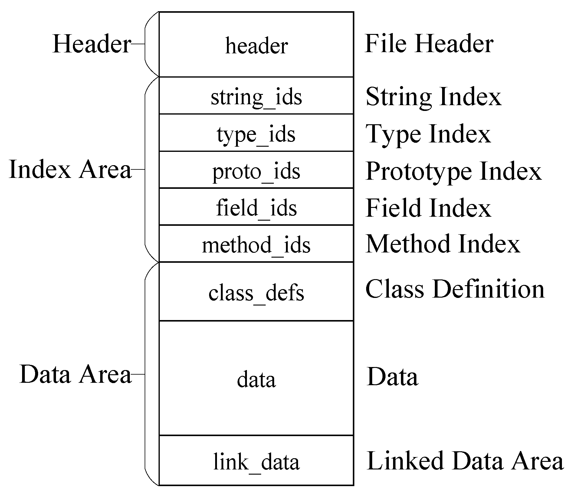
3.3. Base Model for Identifying Android Malware by Dex Header
3.4. Base Model for Identifying Android Malware by Power Spectral Density of Structural Entropy of Dex File
| Algorithm 1: Calculate the structural entropy sequences using Shannon entropy |
 |
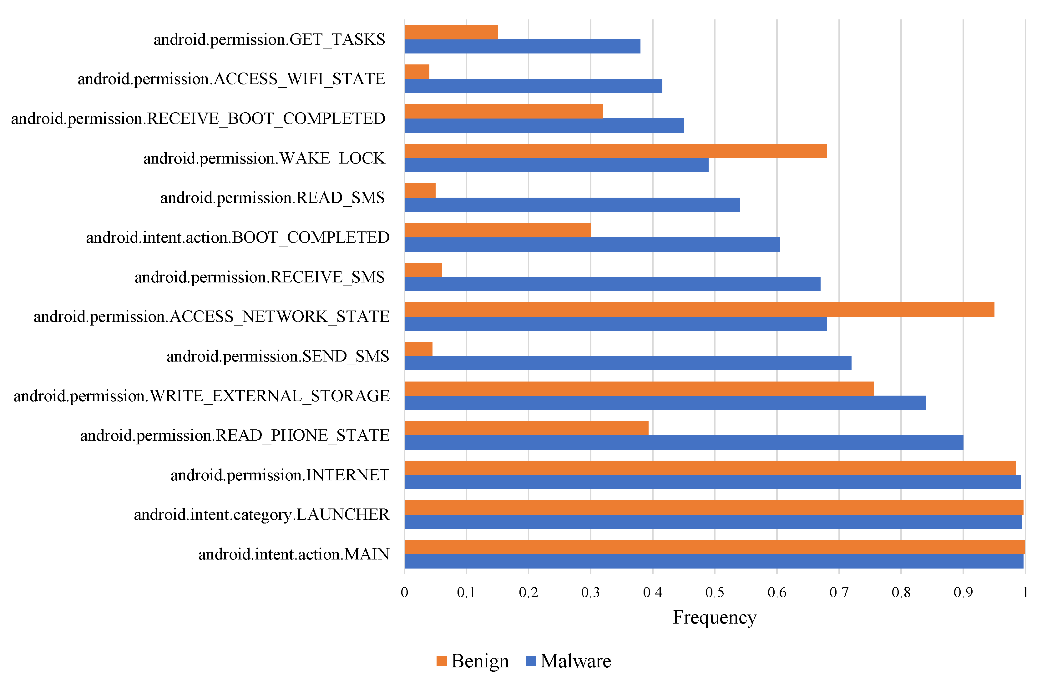
3.5. Base Model for Identifying Android Malware by Permission and Intent
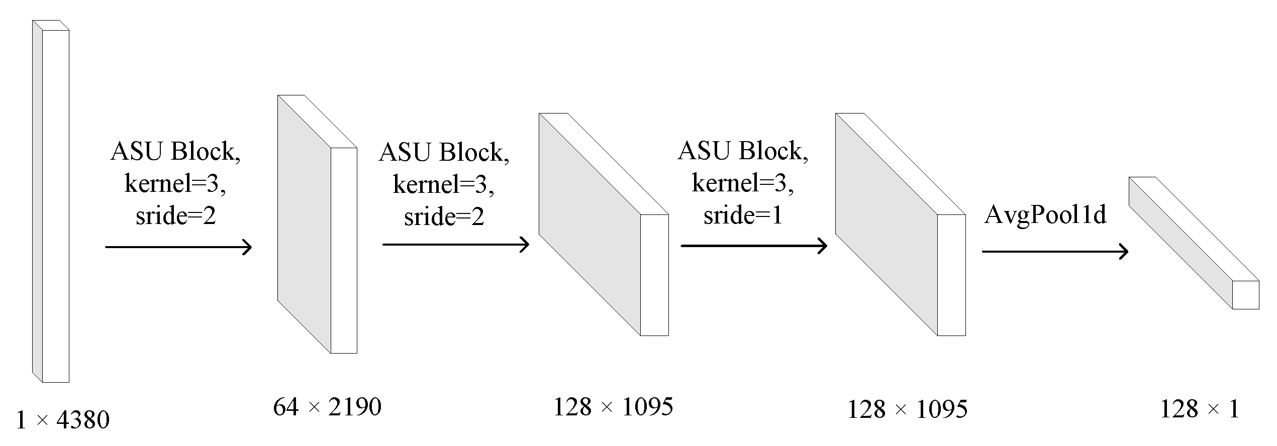
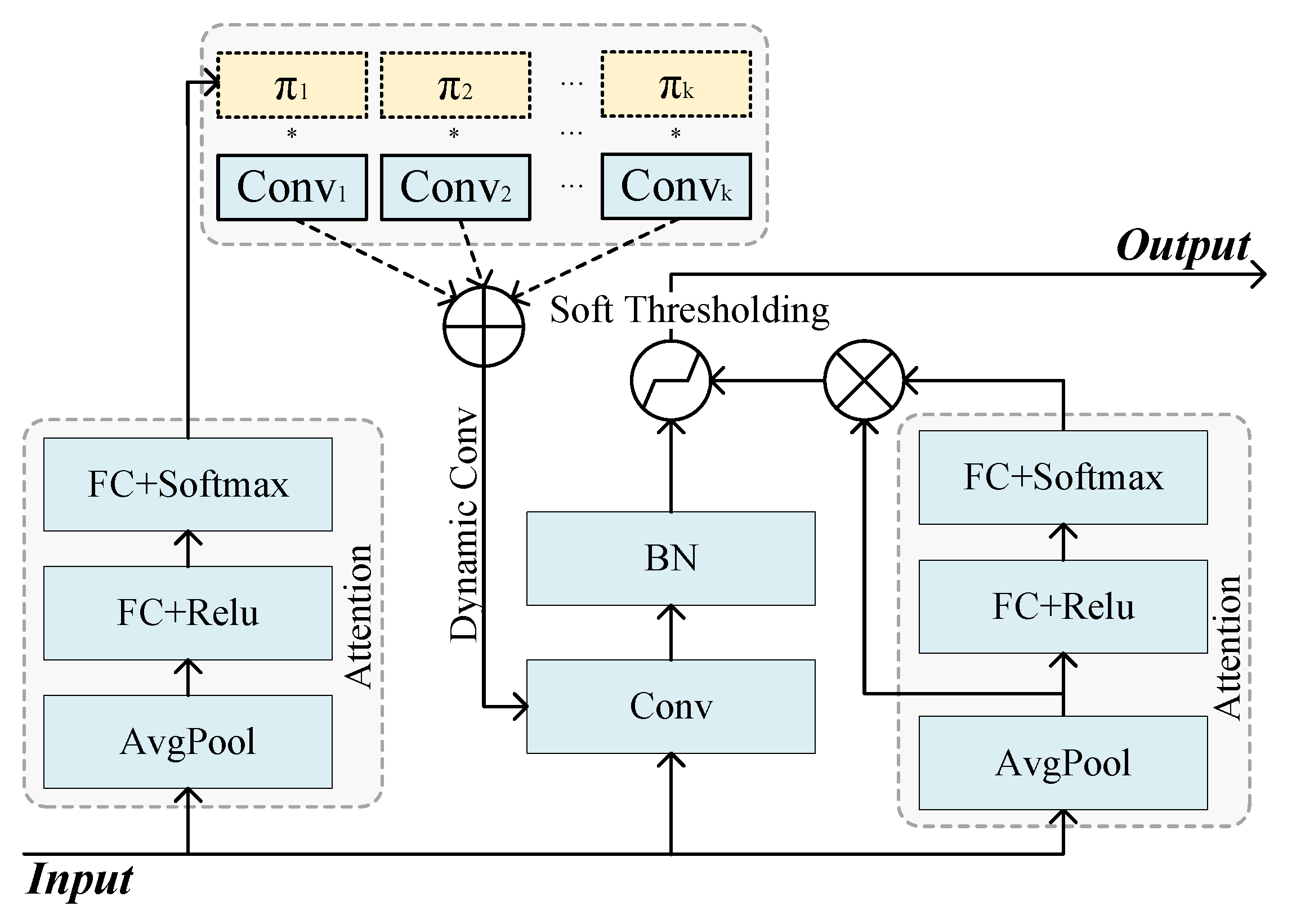
3.6. Adaptive Shrinkage Convolution Unit
3.7. Adaptive Soft Voting Ensemble Method
4. Experimental Results and Analysis
4.1. Dataset
4.2. Experimental Setup
4.3. Comparison of Different Methods
- Meenu’s method: CNN-Based Android Malware Detection [41]. It Extracts permission information from AndroidManifest.xml, encodes it into a permission vector, and extracts features using LeNet.
- XushengXiao’s method: An Image-Inspired and CNN-Based Android Malware Detection Approach [42]. It reads Dalvik bytecode in hexadecimal, transforms it into a three-channel color matrix, and extracts features using CNN.
- Muhammad’s method: Static Malware Detection and Attribution in Android Byte-code through an End-to-End Deep System [43]. It proposes an end-to-end network to detect the byte-code of an application by using a bidirectional LSTM on the extracted opcodes to detect Android malware by using bi-directional LSTM.
- David’s method: EntropLyzer: Android Malware Classification and Characterization Using Entropy Analysis of Dynamic Characteristics [44]. It proposes an entropy-based behavior analysis technique using memory, API, network, Logcat, and battery dynamic characteristics to classify and characterize Android malware.
- XushengWang’s method: MFDroid: A Stacking Ensemble Learning Framework for Android Malware Detection [13]. It uses seven feature selection algorithms to select permissions, API calls and opcodes, then merges the results of each feature selection algorithm to obtain a new feature set, and subsequently uses logistic regression to obtain classification results.
- Mahindru’s method: HybriDroid: an empirical analysis on efective malware detection model developed using ensemble methods [12]. It applies five distinct machine learning algorithms and non-linear ensemble decision tree forest to detect malware in Android applications.
- Ahmed’s method: Mitigating adversarial evasion attacks of ransomware using ensemble learning [25]. It proposes an hybrid analysis approach to detect Android malware by monitoring memory usage, system call logs and CPU usage, statically and dynamically checking permissions, text and network-based functions.
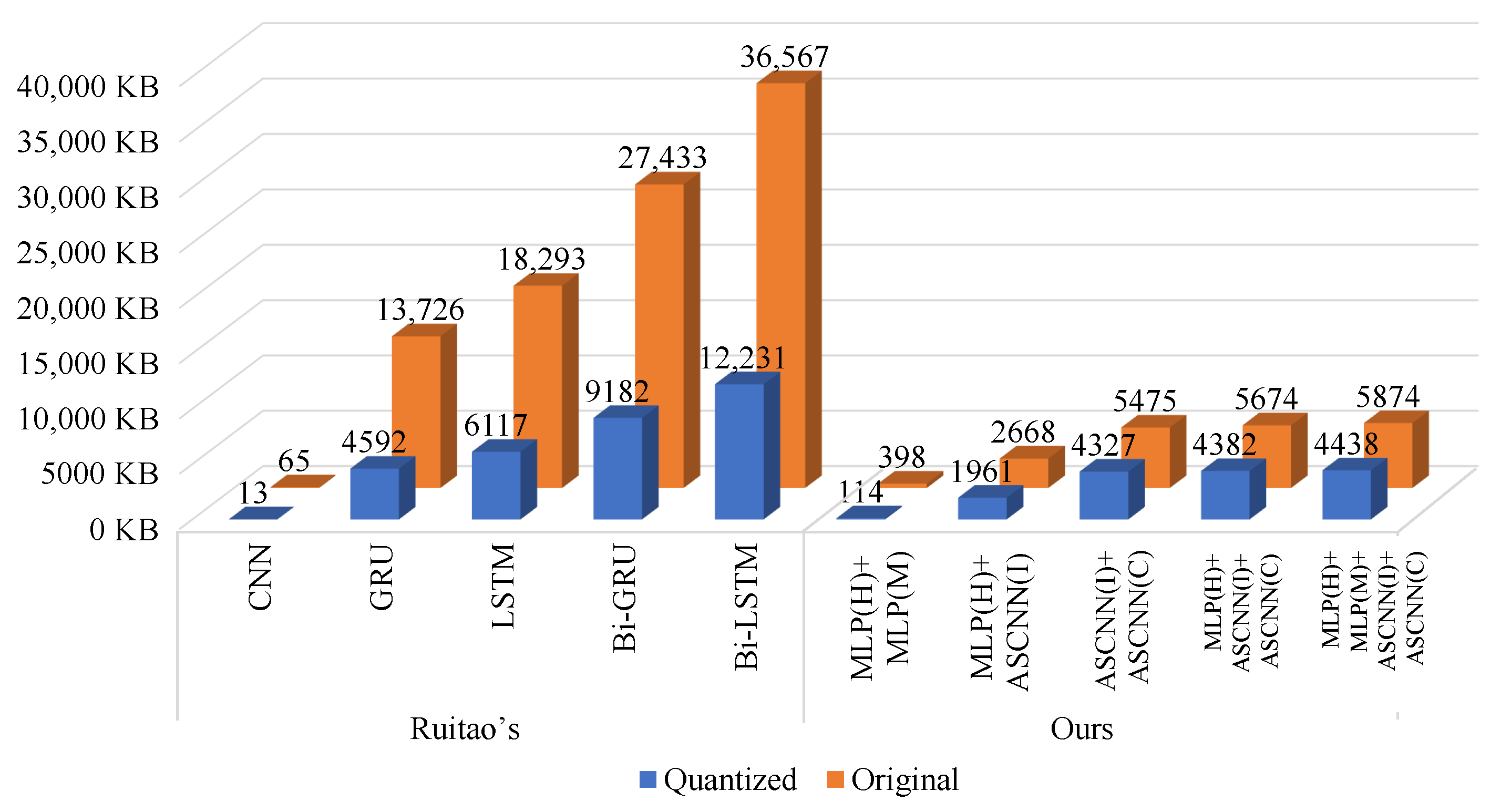
- Ruitao’s method: A Performance-Sensitive Malware Detection System Using Deep Learning on Mobile Devices [5]. It proposes a fast malware detection method by extracting manifest properties and API calls directly from the binary code of an Android application and vectorizing them, and finally using a quantized neural network.
4.4. Comparison with Anti-Virus Softwares
4.5. Analysis of Experimental Results
4.5.1. A Study on the Performance of Adaptive Shrinkage Convolution
4.5.2. A Study on the Performance of Adaptive Soft Voting Method
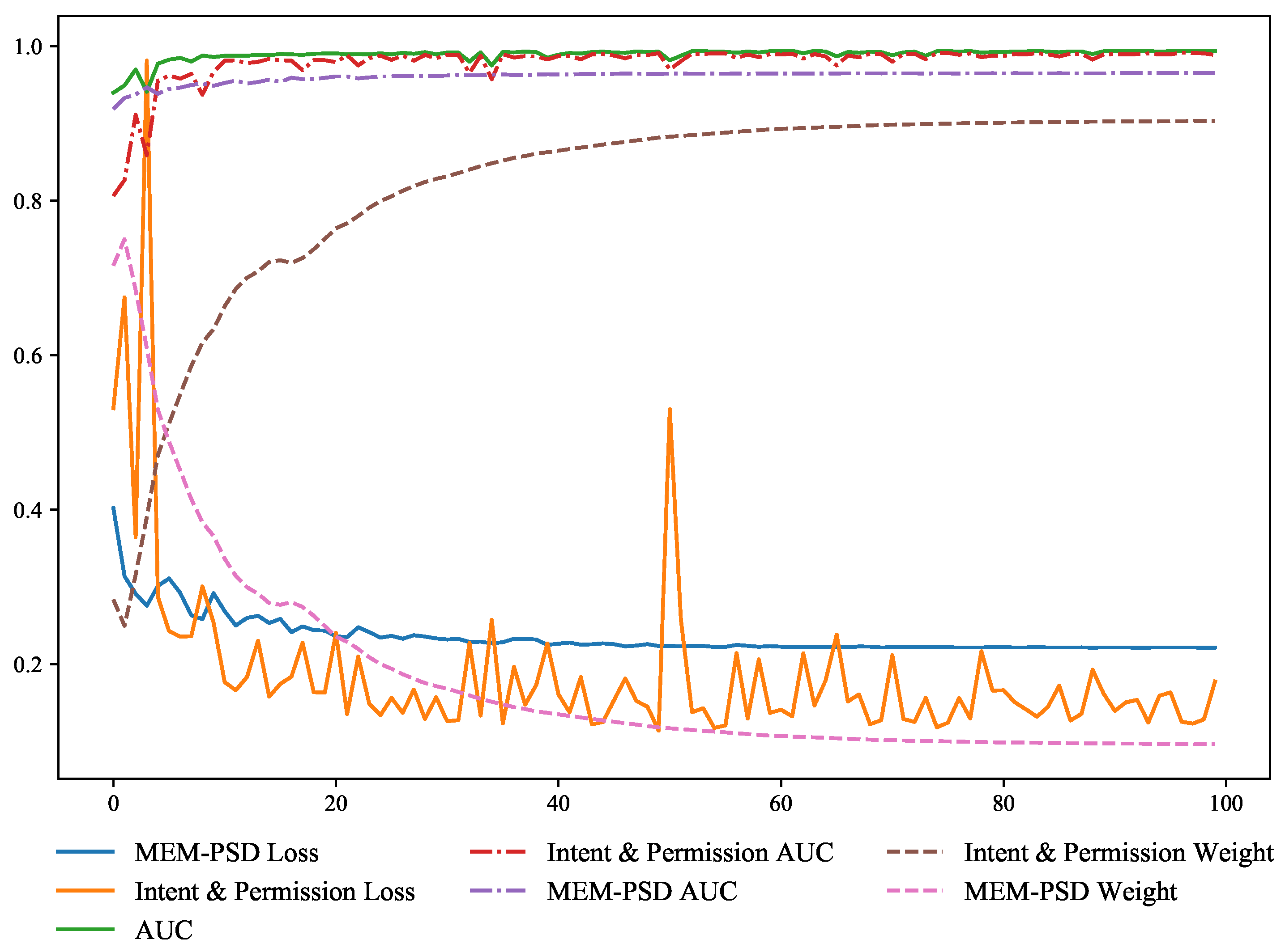
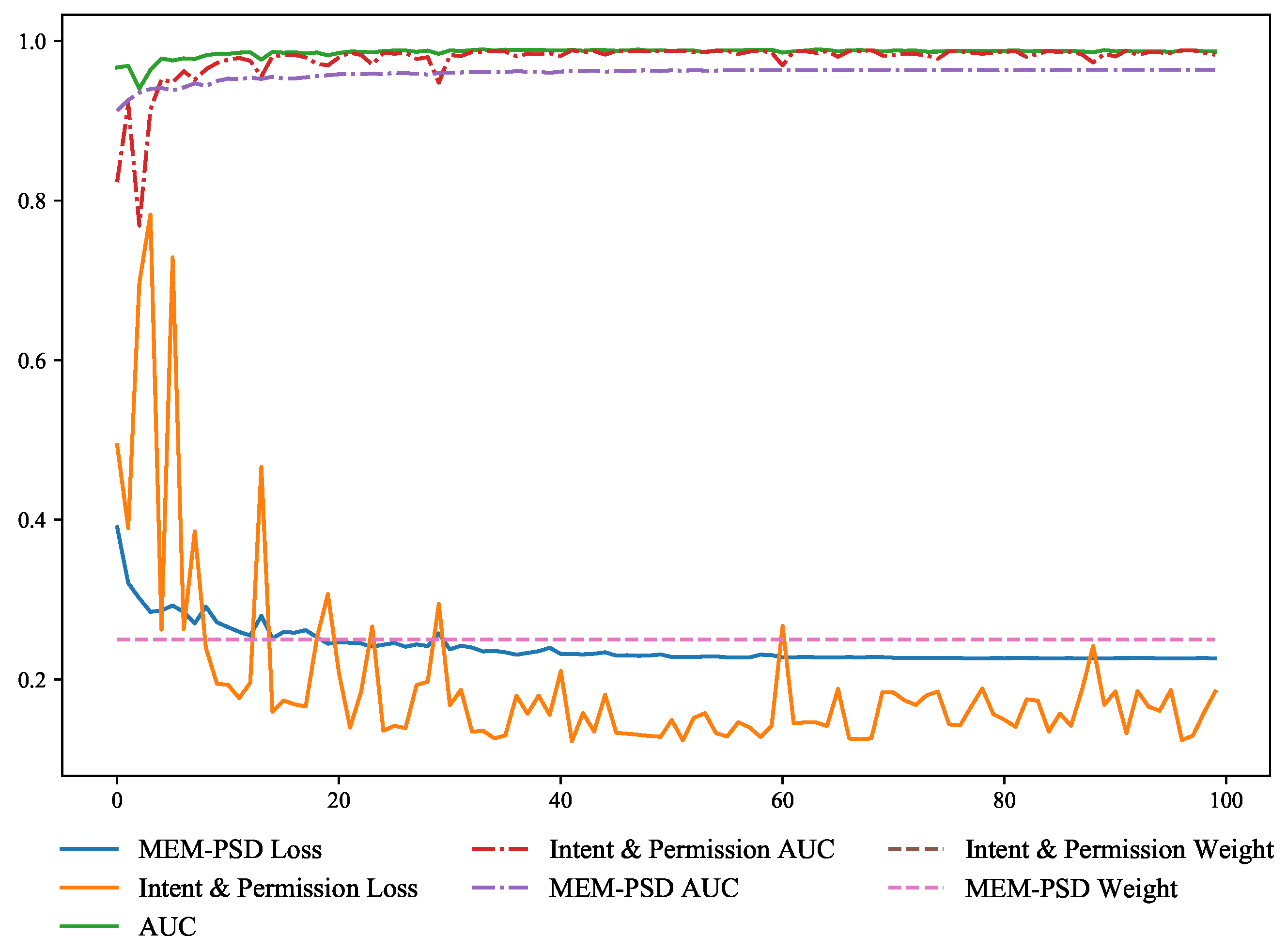
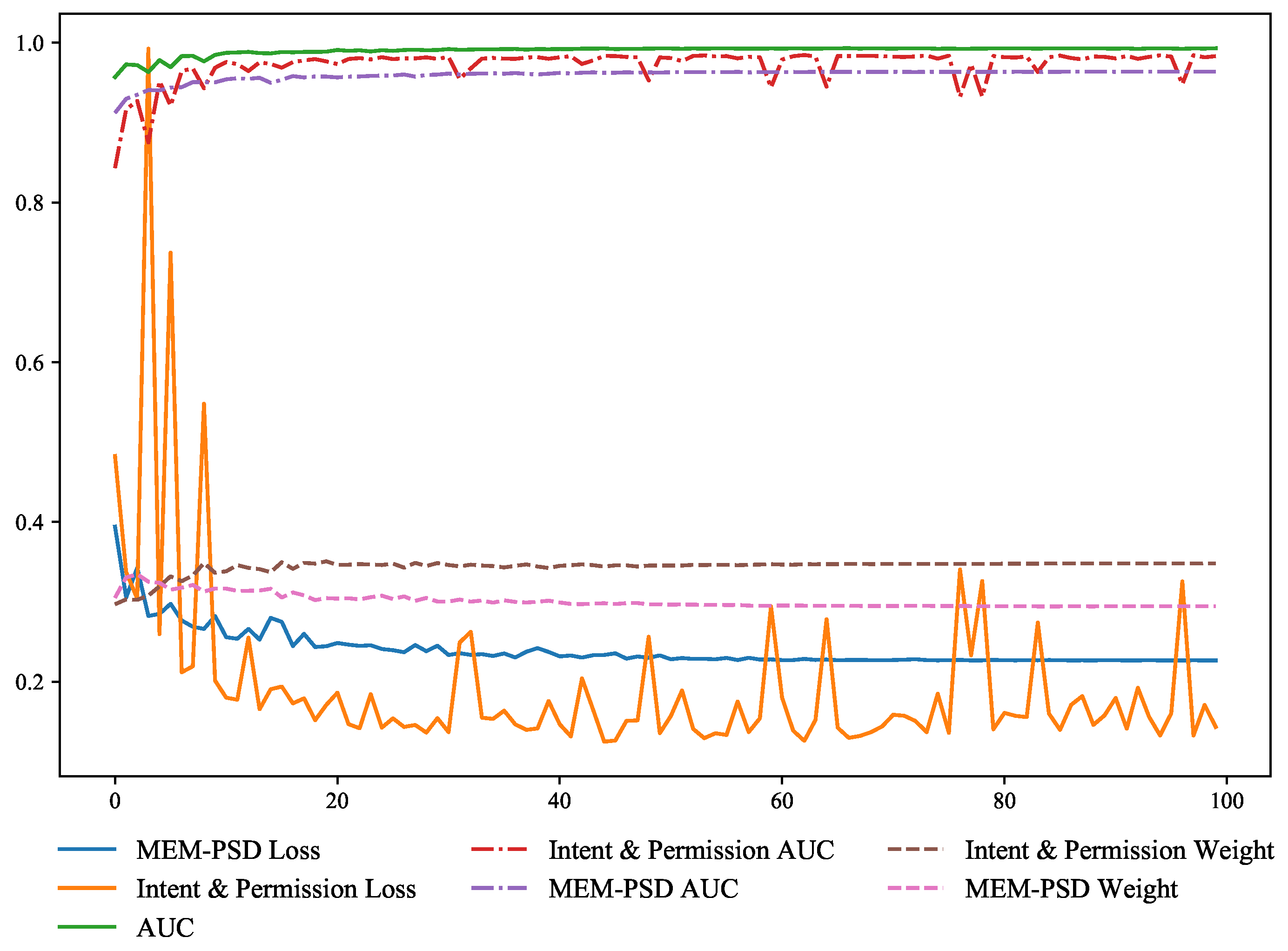
4.5.3. A Study of Weighting Parameter in Adaptive Soft Voting Loss Functions
5. Conclusions and Future Work
Author Contributions
Funding
Institutional Review Board Statement
Informed Consent Statement
Data Availability Statement
Acknowledgments
Conflicts of Interest
Abbreviations
| MEM-PSD | Power spectral density calculated by maximum entropy method |
| AdaSV | Adaptive soft voting |
| ASCNN | Adaptive shrinkage convolutional neural network |
| MLP | Multilayer perceptron |
| H | Dex head feature |
| M | Power spectral density feature of entropy sequence of the Dex file |
| I | APK’s permission and intent feature |
| C | Combined features of Dex head features and power spectral density features of entropy sequences of Dex files |
References
- 2020 Android Platform Security Situation Analysis Report. Available online: https://www.qianxin.com/threat/reportdetail?report_id=125 (accessed on 2 April 2022).
- O’Dea, S. Market Share of Mobile Operating Systems Worldwide 2012–2021. Available online: https://www.statista.com/statistics/272698/ (accessed on 2 April 2022).
- Liu, K.; Xu, S.; Xu, G.; Zhang, M.; Sun, D.; Liu, H. A review of android malware detection approaches based on machine learning. IEEE Access 2020, 8, 124579–124607. [Google Scholar] [CrossRef]
- Wang, B.; Yao, Y.; Shan, S.; Li, H.; Viswanath, B.; Zheng, H.; Zhao, B.Y. Neural cleanse: Identifying and mitigating backdoor attacks in neural networks. In Proceedings of the 2019 IEEE Symposium on Security and Privacy (SP), San Francisco, CA, USA, 19–23 May 2019; pp. 707–723. [Google Scholar]
- Feng, R.; Chen, S.; Xie, X.; Meng, G.; Lin, S.W.; Liu, Y. A performance-sensitive malware detection system using deep learning on mobile devices. IEEE Trans. Inf. Forensics Secur. 2020, 16, 1563–1578. [Google Scholar] [CrossRef]
- Aslan, Ö.A.; Samet, R. A comprehensive review on malware detection approaches. IEEE Access 2020, 8, 6249–6271. [Google Scholar] [CrossRef]
- LeCun, Y.; Bengio, Y.; Hinton, G. Deep learning. Nature 2015, 521, 436–444. [Google Scholar] [CrossRef] [PubMed]
- Zhao, Y.; Li, L.; Wang, H.; Cai, H.; Bissyandé, T.F.; Klein, J.; Grundy, J. On the Impact of Sample Duplication in Machine-Learning-Based Android Malware Detection. ACM Trans. Softw. Eng. Methodol. (TOSEM) 2021, 30, 1–38. [Google Scholar] [CrossRef]
- Tam, K.; Feizollah, A.; Anuar, N.B.; Salleh, R.; Cavallaro, L. The evolution of android malware and android analysis techniques. ACM Comput. Surv. (CSUR) 2017, 49, 1–41. [Google Scholar] [CrossRef] [Green Version]
- Arp, D.; Spreitzenbarth, M.; Hubner, M.; Gascon, H.; Rieck, K.; Siemens, C. Drebin: Effective and explainable detection of android malware in your pocket. NDSS 2014, 14, 23–26. [Google Scholar]
- Zachariah, R.; Akash, K.; Yousef, M.S.; Chacko, A.M. Android malware detection a survey. In Proceedings of the 2017 IEEE International Conference on Circuits and Systems (ICCS), Thiruvananthapuram, India, 20–21 December 2017; pp. 238–244. [Google Scholar]
- Mahindru, A.; Sangal, A. HybriDroid: An empirical analysis on effective malware detection model developed using ensemble methods. J. Supercomput. 2021, 77, 8209–8251. [Google Scholar] [CrossRef]
- Wang, X.; Zhang, L.; Zhao, K.; Ding, X.; Yu, M. MFDroid: A Stacking Ensemble Learning Framework for Android Malware Detection. Sensors 2022, 22, 2597. [Google Scholar] [CrossRef]
- Pan, Y.; Ge, X.; Fang, C.; Fan, Y. A systematic literature review of android malware detection using static analysis. IEEE Access 2020, 8, 116363–116379. [Google Scholar] [CrossRef]
- Choudhary, S.R.; Gorla, A.; Orso, A. Automated test input generation for android: Are we there yet?(e). In Proceedings of the 2015 30th IEEE/ACM International Conference on Automated Software Engineering (ASE), Lincoln, NE, USA, 9–13 November 2015; pp. 429–440. [Google Scholar]
- Bläsing, T.; Batyuk, L.; Schmidt, A.D.; Camtepe, S.A.; Albayrak, S. An android application sandbox system for suspicious software detection. In Proceedings of the 2010 5th International Conference on Malicious and Unwanted Software, Nancy, France, 19–20 October 2010; pp. 55–62. [Google Scholar]
- Wong, M.Y.; Lie, D. IntelliDroid: A Targeted Input Generator for the Dynamic Analysis of Android Malware. NDSS 2016, 16, 21–24. [Google Scholar]
- Dixon, B.; Jiang, Y.; Jaiantilal, A.; Mishra, S. Location based power analysis to detect malicious code in smartphones. In Proceedings of the 1st ACM Workshop on Security and Privacy in Smartphones and Mobile Devices, Chicago, IL, USA, 17 October 2011; pp. 27–32. [Google Scholar]
- Kim, H.; Smith, J.; Shin, K.G. Detecting energy-greedy anomalies and mobile malware variants. In Proceedings of the 6th International Conference on Mobile Systems, Applications, and Services, Breckenridge, CO, USA, 17–20 June 2008; pp. 239–252. [Google Scholar]
- Shabtai, A.; Kanonov, U.; Elovici, Y.; Glezer, C.; Weiss, Y. “Andromaly”: A behavioral malware detection framework for android devices. J. Intell. Inf. Syst. 2012, 38, 161–190. [Google Scholar] [CrossRef]
- Ding, C.; Luktarhan, N.; Lu, B.; Zhang, W. A Hybrid Analysis-Based Approach to Android Malware Family Classification. Entropy 2021, 23, 1009. [Google Scholar] [CrossRef]
- Arora, A.; Garg, S.; Peddoju, S.K. Malware detection using network traffic analysis in android based mobile devices. In Proceedings of the 2014 Eighth International Conference on Next Generation Mobile Apps, Services and Technologies, Oxford, UK, 10–12 September 2014; pp. 66–71. [Google Scholar]
- Ali-Gombe, A.I.; Saltaformaggio, B.; Xu, D.; Richard, G.G., III. Toward a more dependable hybrid analysis of android malware using aspect-oriented programming. Comput. Secur. 2018, 73, 235–248. [Google Scholar] [CrossRef]
- Arshad, S.; Shah, M.A.; Wahid, A.; Mehmood, A.; Song, H.; Yu, H. SAMADroid: A novel 3-level hybrid malware detection model for android operating system. IEEE Access 2018, 6, 4321–4339. [Google Scholar] [CrossRef]
- Ahmed, U.; Lin, J.C.W.; Srivastava, G. Mitigating adversarial evasion attacks of ransomware using ensemble learning. Comput. Electr. Eng. 2022, 100, 107903. [Google Scholar] [CrossRef]
- Wang, H.; Li, Y.; Guo, Y.; Agarwal, Y.; Hong, J.I. Understanding the purpose of permission use in mobile apps. ACM Trans. Inf. Syst. (TOIS) 2017, 35, 1–40. [Google Scholar] [CrossRef]
- Shafiq, M.Z.; Tabish, S.M.; Mirza, F.; Farooq, M. Pe-miner: Mining structural information to detect malicious executables in realtime. In International Workshop on Recent Advances in Intrusion Detection; Springer: Berlin/Heidelberg, Germany, 2009; pp. 121–141. [Google Scholar]
- Wojnowicz, M.; Chisholm, G.; Wolff, M.; Zhao, X. Wavelet decomposition of software entropy reveals symptoms of malicious code. J. Innov. Digit. Ecosyst. 2016, 3, 130–140. [Google Scholar] [CrossRef]
- Liu, L.; He, X.; Liu, L.; Qing, L.; Fang, Y.; Liu, J. Capturing the symptoms of malicious code in electronic documents by file’s entropy signal combined with machine learning. Appl. Soft Comput. 2019, 82, 105598. [Google Scholar] [CrossRef] [Green Version]
- Jwo, D.J.; Wu, I.H.; Chang, Y. Windowing Design and Performance Assessment for Mitigation of Spectrum Leakage. E3S Web Conf. 2019, 94, 03001. [Google Scholar] [CrossRef]
- Bertocci, U.; Frydman, J.; Gabrielli, C.; Huet, F.; Keddam, M. Analysis of electrochemical noise by power spectral density applied to corrosion studies: Maximum entropy method or fast Fourier transform? J. Electrochem. Soc. 1998, 145, 2780. [Google Scholar] [CrossRef]
- Tanaka, Y. Nonlinear time series analysis; the construction of a data analysis system’Memcalc’. Bull Fac. Engin. Hokkaido Univ. 1992, 160, 11–23. [Google Scholar]
- Childers, D.G. Modern Spectrum Analysis; IEEE Computer Society Press: Piscataway, NJ, USA, 1978. [Google Scholar]
- Kumar, R.; Zhang, X.; Khan, R.U.; Sharif, A. Research on data mining of permission-induced risk for android IoT devices. Appl. Sci. 2019, 9, 277. [Google Scholar] [CrossRef] [Green Version]
- Chen, H.; Su, J.; Qiao, L.; Xin, Q. Malware collusion attack against SVM: Issues and countermeasures. Appl. Sci. 2018, 8, 1718. [Google Scholar] [CrossRef] [Green Version]
- Chen, Y.; Dai, X.; Liu, M.; Chen, D.; Yuan, L.; Liu, Z. Dynamic convolution: Attention over convolution kernels. In Proceedings of the IEEE/CVF Conference on Computer Vision and Pattern Recognition, Seattle, WA, USA, 13–19 June 2020; pp. 11030–11039. [Google Scholar]
- Zhang, Y.; Zhang, J.; Wang, Q.; Zhong, Z. Dynet: Dynamic convolution for accelerating convolutional neural networks. arXiv 2020, arXiv:2004.10694. [Google Scholar]
- Zhao, M.; Zhong, S.; Fu, X.; Tang, B.; Pecht, M. Deep residual shrinkage networks for fault diagnosis. IEEE Trans. Ind. Inform. 2019, 16, 4681–4690. [Google Scholar] [CrossRef]
- CICMalDroid 2020. Available online: https://www.unb.ca/cic/datasets/maldroid-2020.html (accessed on 2 April 2022).
- Investigation of the Android Malware (CIC-InvesAndMal2019). Available online: https://www.unb.ca/cic/datasets/invesandmal2019.html (accessed on 2 April 2022).
- Ganesh, M.; Pednekar, P.; Prabhuswamy, P.; Nair, D.S.; Park, Y.; Jeon, H. CNN-based android malware detection. In Proceedings of the 2017 International Conference on Software Security and Assurance (ICSSA), Altoona, PA, USA, 24–25 July 2017; pp. 60–65. [Google Scholar]
- Xiao, X.; Yang, S. An image-inspired and cnn-based android malware detection approach. In Proceedings of the 2019 34th IEEE/ACM International Conference on Automated Software Engineering (ASE), San Diego, CA, USA, 11–15 November 2019; pp. 1259–1261. [Google Scholar]
- Amin, M.; Tanveer, T.A.; Tehseen, M.; Khan, M.; Khan, F.A.; Anwar, S. Static malware detection and attribution in android byte-code through an end-to-end deep system. Future Gener. Comput. Syst. 2020, 102, 112–126. [Google Scholar] [CrossRef]
- Keyes, D.S.; Li, B.; Kaur, G.; Lashkari, A.H.; Gagnon, F.; Massicotte, F. EntropLyzer: Android Malware Classification and Characterization Using Entropy Analysis of Dynamic Characteristics. In Proceedings of the 2021 Reconciling Data Analytics, Automation, Privacy, and Security: A Big Data Challenge (RDAAPS), Hamilton, ON, Canada, 18–19 May 2021; pp. 1–12. [Google Scholar]


| Method | AUC | ACC | F1-Score | Average Time Consumption on PC |
|---|---|---|---|---|
| Meenu’s [41] | 95.36% | 93.67% | 94.53% | 0.64 s |
| XushengXiao’s [42] | 94.34% | 93.00% | 94.02% | 0.22 s |
| XushengWang’s [13] | 97.66% | 96.35% | 96.10% | 0.21 s |
| Muhammad’s [43] | 98.82% | 99.92% | 98.35% | 0.35 s |
| David’s [44] | 99.06% | 98.42% | 98.20% | - |
| Mahindru’s [12] | 98.95% | 98.53% | 96.72% | 0.15 s |
| Ahmed’s [25] | 99.38% | 98.77% | 98.12% | - |
| Ruitao’s [5] | 97.06% | 96.75% | 96.91% | 0.19 s |
| MSFDroid | 99.52% | 97.26% | 97.89% | 0.14 s |
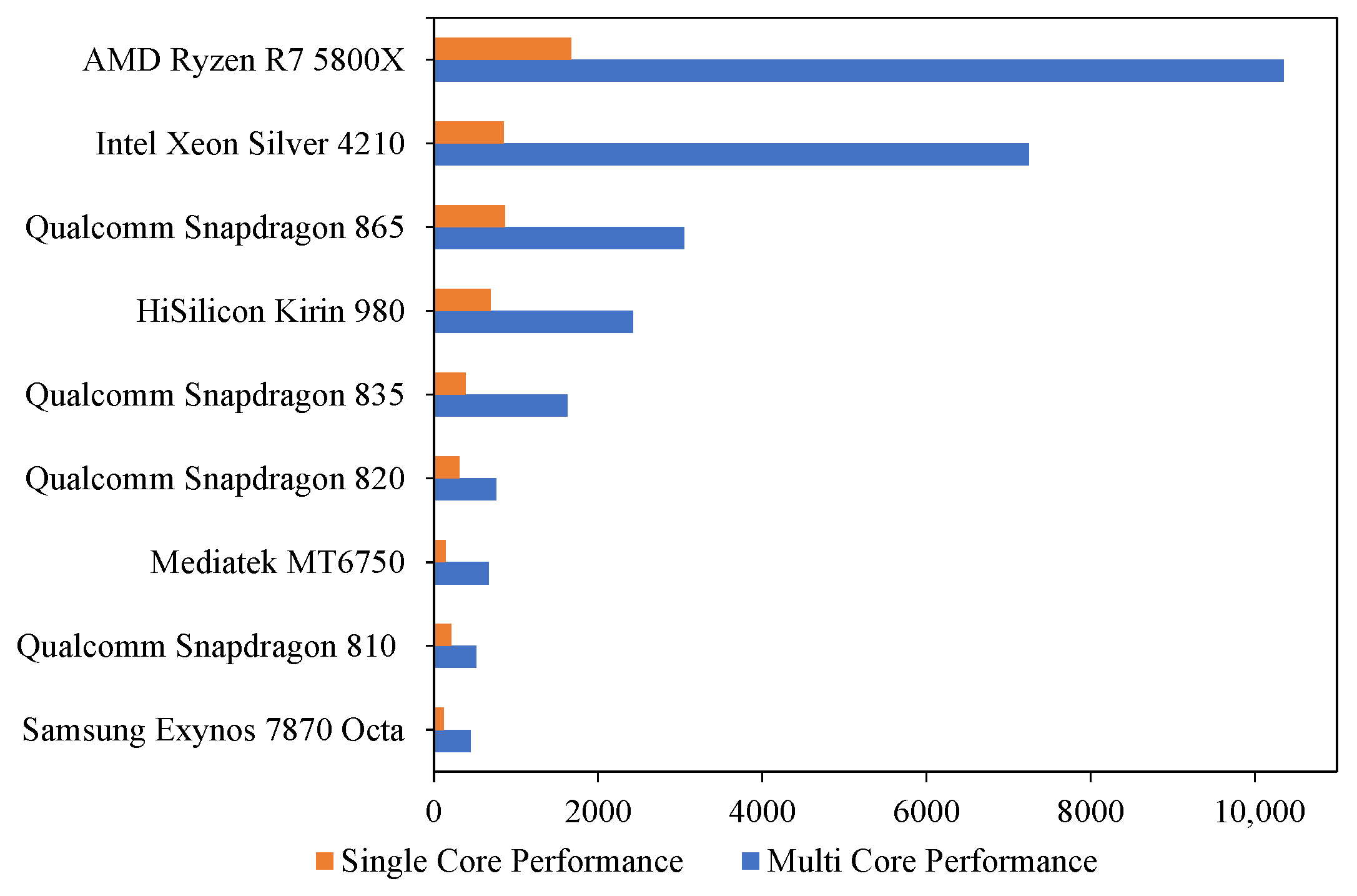
| Device | CPU | Time Consumption | ||
|---|---|---|---|---|
| Model | Performance | MSFDroid | Ruitao’s [5] | |
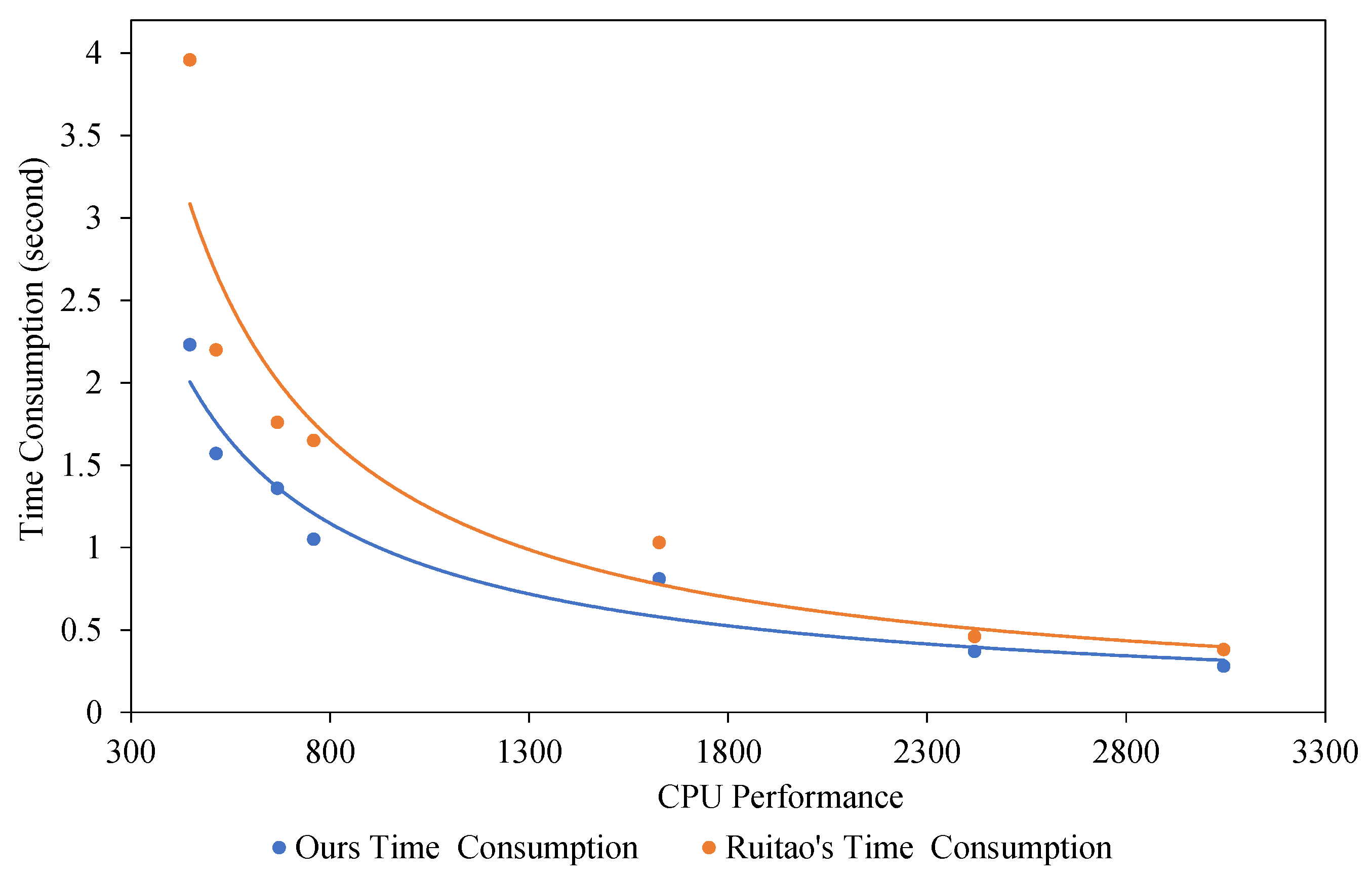
| Galaxy J7 Pro | Exynos 7870 Octa | 448 | 2.33 s | 3.96 s |
| Nexux 6P | Qualcomm Snapdragon 810 | 514 | 1.57 s | 2.20 s |
| Oppo F3 | Mediatek MT6750 | 668 | 1.36 s | 1.76 s |
| OnePlus 3 | Qualcomm Snapdragon 820 | 759 | 1.05 s | 1.65 s |
| OnePlus 5T | Qualcomm Snapdragon 835 | 1627 | 0.81 s | 1.03 s |
| Huawei P30 | HiSilicon Kirin 980 | 2419 | 0.37 s | 0.46 s |
| OnePlus 8Pro | Qualcomm Snapdragon 865 | 3045 | 0.28 s | 0.38 s |
| Device | CPU | Arch | Extraction Time | Prediction Time | Total Time |
|---|---|---|---|---|---|
| Galaxy J7 Pro | Exynos 7870 Octa | ARMv8 | 476.85 s | 1758.161 s | 2.232 s |
| Nexus 6P | QCOM Snapdragon 710 | ARMv8 | 392.412 s | 1183.588 ms | 1.575 s |
| Oppo F3 | Mediatek MT6750 | ARMv8 | 375.939 ms | 987.057 ms | 1.363 s |
| OnePlus 3 | QCOM Snapdragon 820 | ARMv8 | 257.021 ms | 793.548 ms | 1.051 s |
| OnePlus 5T | QCOM Snapdragon 835 | ARMv8 | 211.628 ms | 699.563 ms | 0.911 s |
| Huawei P30 | HiSilicon Kirin 980 | ARMv8 | 176.942 ms | 195.222 ms | 0.372 s |
| OnePlus 8Pro | QCOM Snapdragon 865 | ARMv8 | 96.501 ms | 182.123 ms | 0.279 s |
| x64 Server | Intel Xeon Silver 4210 | x86_64 | 67.515 ms | 89.088 ms | 0.157 s |
| x64 PC | AMD Ryzen7 5800X | x86_64 | 58.019 ms | 46.429 ms | 0.104 s |
| Anti-Virus Software | Detection Rate | Average Time Consumption Per Sample |
|---|---|---|
| Huorong | 86.4% | 0.07 s |
| Norton | 93.7% | 0.06 s |
| McAfee | 93.8% | 0.05 s |
| Kaspersky | 94.3% | 0.07 s |
| Avast | 96.7% | 0.05 s |
| MSFDroid | 98.6% | 0.14 s |
| Model | AUC | ACC | F1-Score |
|---|---|---|---|
| 3-layer convolutional neural network | 97.26% | 92.57% | 94.76% |
| 6-layer convolutional neural network | 98.74% | 95.15% | 95.61% |
| 3-layer adaptive shrinkage convolution neural network | 99.23% | 95.28% | 96.29% |
| Integration of Base Models | AUC | ACC | F1-Score |
|---|---|---|---|
| MLP(H) | 95.73% | 83.54% | 81.07% |
| MLP(M) | 96.12% | 88.98% | 91.76% |
| ASCNN(I) | 98.06% | 88.97% | 88.75% |
| MLP(H) + MLP(M) | 97.66% | 94.30% | 95.94% |
| ASCNN(I) + ASCNN(C) | 99.23% | 95.69% | 96.76% |
| MLP(H) + MLP(M) + ASCNN(I) | 99.39% | 96.83% | 97.20% |
| MLP(H) + MLP(M) + ASCNN(I) + ASCNN(C) | 99.52% | 97.26% | 97.89% |
| Integration of Base Models | Ensemble Model | AUC | ACC | F1-Score |
|---|---|---|---|---|
| MLP(H)+MLP(M) | Adaptive Soft Voting () | 97.66% | 94.30% | 95.94% |
| Static Weighted Soft Voting | 97.14% | 93.12% | 95.13% | |
| ASCNN(I)+MLP(M) | Adaptive Soft Voting () | 99.23% | 95.28% | 96.29% |
| Static Weighted Soft Voting | 99.13% | 93.86% | 95.37% | |
| MLP(H)+MLP(M)+MLP(I) | Adaptive Soft Voting () | 99.39% | 96.83% | 97.20% |
| Static Weighted Soft Voting | 99.15% | 94.06% | 95.79% | |
| MLP(H)+MLP(M)+ASCNN(I)+ ASCNN(C) | Adaptive Soft Voting () | 99.52% | 97.26% | 97.89% |
| Static Weighted Soft Voting | 99.09% | 93.49% | 95.42% |
Publisher’s Note: MDPI stays neutral with regard to jurisdictional claims in published maps and institutional affiliations. |
© 2022 by the authors. Licensee MDPI, Basel, Switzerland. This article is an open access article distributed under the terms and conditions of the Creative Commons Attribution (CC BY) license (https://creativecommons.org/licenses/by/4.0/).
Share and Cite
Peng, T.; Hu, B.; Liu, J.; Huang, J.; Zhang, Z.; He, R.; Hu, X. A Lightweight Multi-Source Fast Android Malware Detection Model. Appl. Sci. 2022, 12, 5394. https://doi.org/10.3390/app12115394
Peng T, Hu B, Liu J, Huang J, Zhang Z, He R, Hu X. A Lightweight Multi-Source Fast Android Malware Detection Model. Applied Sciences. 2022; 12(11):5394. https://doi.org/10.3390/app12115394
Chicago/Turabian StylePeng, Tao, Bochao Hu, Junping Liu, Junjie Huang, Zili Zhang, Ruhan He, and Xinrong Hu. 2022. "A Lightweight Multi-Source Fast Android Malware Detection Model" Applied Sciences 12, no. 11: 5394. https://doi.org/10.3390/app12115394
APA StylePeng, T., Hu, B., Liu, J., Huang, J., Zhang, Z., He, R., & Hu, X. (2022). A Lightweight Multi-Source Fast Android Malware Detection Model. Applied Sciences, 12(11), 5394. https://doi.org/10.3390/app12115394