Double-Cycling AGV Scheduling Considering Uncertain Crane Operational Time at Container Terminals

Abstract

Container terminals (CTs) play an important role in the modern logistics and transportation industry. The utilization of automated guided vehicles (AGVs) can be effectively facilitated by reducing their empty running. The existing strategies cannot guarantee the full load of AGVs during their transportation because of the complex constraints of container scheduling. This work proposes a double-cycling AGV scheduling model that ensures a full load of AGVs between the quayside and the yard. The objective is to minimize the total waiting time of AGVs and ensure a high loading rate of AGVs by scheduling loading/unloading containers. Furthermore, it takes the randomness of the quay crane’s operational time into consideration. By assigning a time interval to AGVs’ arrival at a quayside, a container scheduling sequence is obtained based on a Hybrid Particle Swarm Optimization (HPSO) algorithm with a penalty function. Via experiments, it shows that the proposed model can obtain the least number of AGVs for container transportation, minimize AGVs’ total waiting time, and ensure the high loading rate of AGVs.

1. Introduction

Maritime transportation plays a vital role in the global economy, trade, and cultural exchanges as a basic logistic mode. Container terminals (CTs) were developed as one of the most critical components in logistic transportation systems. CTs consist of three major facilities: quay cranes (QCs), yard cranes (YCs), and automated guided vehicles (AGVs). AGVs cooperate with QC and YC operations. Effective task scheduling of AGVs is the key to reducing the operating cost of CTs. In the terminal’s traditional transportation mode, it is essential to ensure the working efficiency of the quay crane. Most terminals use more AGVs to avoid waiting for the quay crane. However, this will increase the waiting time of AGVs, thus reducing their utilization rate. Furthermore, the complex constraints among quay cranes, yard cranes, and AGVs further deteriorate the utilization of AGVs.

Many studies focused on the real-time scheduling of AGVs over the past few decades. For example, Mohammad and Saeed proposed a mathematical model composed of a job shop scheduling problem and a conflict-free routing problem [1]. The objective was to minimize AGVs’ delay time and achieve multi-AGV integrated scheduling. A two-stage ant colony algorithm was proposed to solve it. Angeloudis and Bell studied job assignments of AGVs in CTs under various uncertainty conditions [2]. A flexible algorithm for real-time AGV scheduling was proposed. Luo et al. designed an algorithm to prevent AGVs from collisions based on labeled Petri nets [3]. Ji et al. studied the combinatorial optimization of two problems in the synchronous loading and unloading operation mode of the automated container terminal. They designed two bi-level optimization algorithms based on a conflict resolution strategy [4]. Wang and Zeng investigated the AGV dispatching and routing problem with multiple bidirectional paths to generate conflict-free routes. A mixed-integer programming model was formulated to minimize the completion time of all jobs. A tailored branch-and-bound algorithm was developed to solve the problem [5]. Zhong et al. studied a conflict-free AGV path planning problem and rail-mounted gantry crane scheduling problem [6].

In terms of AGVs’ offline path planning, Graziana et al. showed how timed Petri nets can be efficiently used to solve problems related to resource planning in intermodal freight transport terminals. They considered a real case study and simulated it based on the timed Petri net model of the terminal [7]. Rashidi and Tsang formulated an AGV scheduling problem as a least-cost flow model [8]. They proposed an extended Network Simplex Algorithm (NSA+). Hu et al. analyzed a container-cluster operation and an optimal scheduling strategy of the yard truck [9]. A multi-objective mathematical programming model was established and then solved by a genetic algorithm. Niu et al. proposed a cooperative strategy for scheduling trucks to minimize the total delay time of requests and the travel time of yard trucks [10]. They applied a particle swarm optimization algorithm to solve the problem. The studies, as mentioned above, significantly improved the utilization of AGVs and the operational efficiency of CTs, but they cannot guarantee a full load and ensure the least total waiting time of AGVs during their transportation. Hence, we propose a double-cycling AGV route planning model in this work to maximize the loading rate and minimize the waiting time of AGVs during their transportation.

In CTs, AGVs cooperate with the working of QCs and YCs. The work efficiency of QCs directly affects the berth time, which is also an important research topic. Many studies focused on an efficient quay crane scheduling problem (QCSP) under various complex conditions. Huang and Li proposed a bounded two-level dynamic programming algorithm aiming at a QCSP [11]. A method was proposed to evaluate the practicability of the algorithm. Ji et al. considered optimizing a loading sequence in CTs [12]. A model was established to integrate the loading sequence and a rehandling strategy under parallel operations of multi-quay cranes. An improved genetic algorithm was proposed to solve the model. Zhang and Kim attempted to minimize the operational cycle time of a QC for unloading and loading containers in a ship bay [13]. They formulated a QCSP as a mixed-integer programming model and solved it using a hybrid heuristic approach. Nguyen and Kim compared various pooling strategies for constructing the pool [14]. Heuristic algorithms were evaluated in terms of the total delay time of QC operations and the total travel distance of AGVs. Zhen et al. studied an integrated optimization QCSP and yard truck scheduling problem (YTSP) in CTs [15]. A mixed-integer programming model was formulated and solved by a particle swarm optimization-based method. Zhang et al. extended the QCSP by considering the stability of containers and proposed a QCSP with stability constraints [16]. A bi-criteria evolutionary algorithm was proposed to solve it. Most of the above QC scheduling methods fail to consider the impact of uncertain factors, especially the tide fluctuation and manual operation, on QC transportation tasks, with a few exceptions (Zhen, 2014 [17]; Sheikholeslami and Ilati, 2018 [18]). Uncertainties can be good or bad for a transportation system (Wang and Wu, 2021 [19]), and we analyze uncertainties in our model.

The dispatch of YCs is another crucial part of CTs. Most researchers combine the scheduling of YCs and AGVs to formulate the model closer to reality. Zheng et al. investigated single YC scheduling to minimize the total tardiness of tasks and focus on the case with uncertain release times of retrieval tasks [20]. A two-stage stochastic programming model was proposed, and a genetic algorithm and a rule-based heuristic were developed to solve it, especially for large-scale instances. Ng and Mak studied the scheduling of a YC to perform a given set of loading and unloading tasks with different ready times, which minimizes the sum of the task waiting time [21]. A branch and bound algorithm was proposed to solve it. Some studies focus on a yard crane scheduling problem (YCSP) under various conditions. Javanshir et al. studied a YCSP among different blocks in CTs to minimize cranes’ total travel time and the total delayed workload [22]. It was formulated as a mixed-integer programming model and solved by a branch-bound method. He et al. addressed a YCSP with the uncertainty about the vessels’ arrival time and volumes [23]. It optimized the total delay to the estimated ending time of all task groups based on a genetic algorithm-based framework combined with a three-stage algorithm.

In CTs, a double-cycling scheduling model of QCs and YCs requires that a crane transports a container, unloads it, and returns by taking another container. Meanwhile, AGVs transport a container to its destination and bring another one back. At present, double-cycling strategies are used in QCSP, YCSP, YTSP, and sequencing the loading of the container (i.e., Container Sequencing Problem, CSP, which refers to sequencing the loading/unloading of the container in the yard [24]), as shown in Table 1. Most of these studies considering a double-cycling scheduling mode do not specifically consider the uncertainty of QC operation. Most of these studies do not obtain specific AGV scheduling, including which containers should be transported by each AGV and the sequence of transporting these containers by an AGV. In this work, a double-cycling model is proposed to realize the full load of AGVs by scheduling loading/unloading containers to minimize the waiting time of the AGVs. A hybrid particle swarm optimization (HPSO) algorithm with a penalty function is used to solve this issue.

Table 1. The problems solved by using double-cycling strategies.

Studies	Scheduling Problem	Uncertainty Considered?	AGV Scheduling Sequence Obtained?
Luo and Wu, 2015 [25]	QCSP with YCSP	No	Yes
Zheng, Pang, Liu, and Xu, 2019 [26]	QCSP with CSP	No	No
Cao et al., 2018 [27]	Integrated QCSP-YTSP	No	Yes
Liu et al., 2015 [28]	QCSP with CSP	No	No
Wang and Li, 2015 [29]	QCSP with CSP	No	No
Nguyen and Kim, 2010 [30]	YTSP	Yes	No
Meisel and Wichmann, 2010 [31]	QCSP with CSP	No	No
Goodchild and Daganzo, 2006 [32]	QCSP	Yes	No
Ahmed, Mohammed, Zayed, Alfalah and Alkass, 2021 [33]	Integrated QCSP-YTSP-YCSP	Yes	No
Our Work	Integrated QCSP-YCSP	Yes	Yes

The rest of this paper is organized as follows. Section 2 describes a double-cycling model and proposes a container scheduling sequence based on an HPSO algorithm. Section 3 shows experimental results. Section 4 concludes this paper and discusses the future work.

2. Materials and Methods

2.1. AGV Double-Cycling

This section describes the double-cycling model. Relevant assumptions are made for QC, AGV, and YC. The related constraints are given.

2.1.1. Problem Description

In a CT, QCs, YCs, and AGVs are, respectively, responsible for loading/unloading containers on ships, loading/unloading containers in the yard, and transporting containers between the quayside and the yard. This work proposes a double-cycling scheduling model. An AGV carries a container at the quayside, drives to the yard to unload it, takes another one from the yard, and returns to the quayside for unloading. Such a process is repeated to finish the handling of containers at CTs. First, we present the following assumptions:

1)

Two QCs are used for loading and unloading containers on ships. One is responsible for loading containers from an AGV to a vessel, and another QC is responsible for unloading containers from a vessel to an AGV. After unloading at the first QC, AGVs run empty to the other QC for loading and finally drive to the yard. After unloading at the yard, AGVs run to the next yard for loading and eventually go to the quayside. Notice that more QCs can be divided into several pairs.

2)

Tidal fluctuation and other factors will cause ship instability, resulting in QC operations not being fully automated. At present, most QC operations need manual assistance, resulting in the uncertainty of QC operation time. Etsuko mentions that the QC operation time roughly conforms to Gaussian distribution [34]. The probability is that the distributed value in (μ − 2σ, μ + 2σ) is 0.9544, so we assume that QC completes the transportation of containers within the time (t + μ − 2σ, t + μ + 2σ), where t is the QC operation time.

3)

AGVs travel at a uniform speed during their transportation.

4)

When transporting a container, the YC and the YC’s spreader are required to reach the position of the container. To save time, YC can be prepared before the arrival of an AGV [35], adopted in our work.

We set up two fixed bays on the ship for storing containers that need to be unloaded and loaded, respectively. Notice that more bays can be divided into several pairs. AGVs are fully loaded in and out of the yard and quayside, thus realizing the double-cycling of AGVs. It is the basic constraint of the model. Figure 1 show the flow chart of this work.

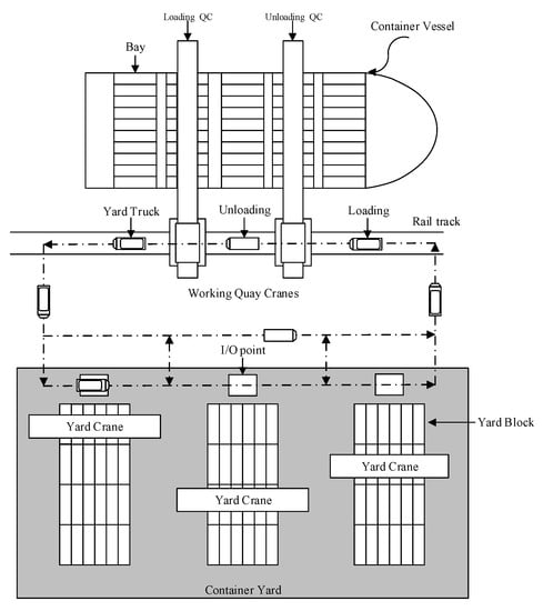
Figure 1. A double-cycling AGV scheduling mode.

The second constraint is that no delay of QCs should be guaranteed. QC operational uncertainty leads to an uncertain time when an AGV arrives at the quayside. The latest time required for an AGV to arrive at the quayside (LTQ) is considered. Because the time of QC transporting containers conforms to the Gaussian distribution with parameters (μ, σ²), LTQ is the moment when the QC finishes the transportation of the previous container.

To make the algorithm and model more concise, we chose task points to represent the transport of containers. A task point represents a container with its current position and destination information. We give a detailed definition of the task point in Section 2.1.2.

2.1.2. Mathematical Model

Let N = {1, 2, … } represent the set of natural numbers, and N_m= {1, 2, …, m}. The related symbols and decision variables are defined as follows in Table 2, Table 3 and Table 4.

Table 2. The symbols and their definitions.

Symbol	Definition
M	$M=\{m_1, m_2, \dots , m_n\} \mathrm{is} \mathrm{a} \mathrm{set} \mathrm{of} \mathrm{task} \mathrm{points}, \mathrm{where} m_i=\left\{P_1^i, w,P_2^i,T_i\right\}$$, n \mathrm{is} \mathrm{the} \mathrm{number} \mathrm{of} \mathrm{task} \mathrm{points}. \mathrm{For} \mathrm{containers} \mathrm{to} \mathrm{be} \mathrm{unloaded} \mathrm{from} \mathrm{ships}, P_1^i$$\mathrm{represents} \mathrm{the} \mathrm{position} \mathrm{of} \mathrm{container} i\mathrm{on} \mathrm{the} \mathrm{ship}, w\mathrm{represents} \mathrm{that} \mathrm{container} i \mathrm{will} \mathrm{be} \mathrm{loaded} \mathrm{at} \mathrm{yard} w, \mathrm{and} P_2^i$$\mathrm{represents} \mathrm{the} \mathrm{destination} \mathrm{of} \mathrm{container} i \mathrm{in} \mathrm{the} \mathrm{yard}. \mathrm{For} \mathrm{containers} \mathrm{to} \mathrm{be} \mathrm{loaded} \mathrm{onto} \mathrm{ships}, P_1^i$$\mathrm{represents} \mathrm{the} \mathrm{destination} \mathrm{of} \mathrm{the} \mathrm{container} \mathrm{in} \mathrm{the} \mathrm{ship}, w\mathrm{represents} \mathrm{that} \mathrm{container} i \mathrm{will} \mathrm{be} \mathrm{unloaded} \mathrm{at} \mathrm{yard} w, \mathrm{and} P_2^i$$\mathrm{represents} \mathrm{the} \mathrm{position} \mathrm{of} \mathrm{container} i\mathrm{on} \mathrm{the} \mathrm{yard}. T_i$ represents the LTQ of container i;
X	a set of unloading task points that represent unloading the containers in the ship onto the yard;
Y	a set of loading task points that represent loading the containers in the yard onto the ship;
l	the number of AGVs;
ag	the g-th AGV where 1 ≤ g ≤ l;
mb	a virtual begin task point;
me	a virtual end task point;
VQ	average movement speed of QC;
$\Delta t_i$	average time of QC spreader grasping container i;
$D_i^q$	the distance that a QC moves to from the position of the AGV to the position of container i;
$C_i$	$\mathrm{a} \mathrm{time}-\mathrm{interval} \mathrm{conforming} \mathrm{to} \mathrm{the} \mathrm{Gaussian} \mathrm{distribution}, \mathrm{including} \mathrm{the} \mathrm{minimum} \mathrm{and} \mathrm{maximum} \mathrm{time} \mathrm{taken} \mathrm{by} \mathrm{QC} \mathrm{to} \mathrm{transport} \mathrm{container} i, \mathrm{where} C{i}_i=(C_1^i$$, C_2^i$$), C_1^i$$\mathrm{and} C_2^i$ are the minimum time and maximum time for QC to transport container i transportation, respectively;
VY	moving speed of YC;
$D_{ij}^Y$	the moving distance of the YC from the position of container i to the position of container j. It represents the distance from the I/O point to the position of container j when i = 0; it represents the distance of the YC moved from the position of container i to the I/O point when j = 0;
Vy	movement speed of spreader;
$D_{ij}^y$	the moving distance of the YC’s spreader from the position of container i to the position of container j. It represents the distance of the spreader moving from the I/O point to the position of container j if i = 0; it represents the distance of the spreader moved from the position of container i to the I/O point if j = 0;
$G_y$	the speed at which the YC’s spreader moves up and down;
di	the distance of the YC’s spreader moves to grab the container i;
$T_i^q$	time taken by QC to transport container i;
$T_y$	time required by the spreader to transport a container at the I/O point;
$T_i^l$	time is taken by YC to load the container i;
$T_i^{ul}$	time is taken by YC to unload the container i;
Tg	Tg ={t1, t2, …, t|Z| + 1}, where tg is the waiting time of ag;
$H_{ij}$	the empty running time of an AGV loading task point mi after unloading task point mj at the yard;
$T$	the time interval between two consecutive AGVs exiting the quayside;
$T_i^{q1}$	the waiting time before task point i is unloaded at the quayside;
$T_i^{q2}$	the waiting time before task point i is loaded at the quayside;
$T_i^1$	the waiting time before task point i is unloaded in the yard;
$T_i^2$	the time taken for task point i to be unloaded in the yard;
$T_i^3$	the waiting time before task point i is loaded in the yard;
$T_i^4$	the time taken for task point i to be loaded in the yard.

Table 3. The symbols used in the algorithm and their definitions.

Symbol	Definition
Q	particle swarm size;
T	current iteration index;
tmax	maximum iteration;
P	particle fitness;
pBest	personal best position, a set of the coding schemes in our algorithm. The personal best position means the optimal scheduling sequence for each particle in the algorithm iteration process;
gBest	global best particle.

Table 4. The decision variables and their definitions.

${\chi }_j^i=\left\{\begin{array}{c}1 , \mathrm{an} \mathrm{AGV} \mathrm{transports} \mathrm{task} \mathrm{point} j \mathrm{after} \mathrm{task} \mathrm{point} i\\ 0, \mathrm{otherwise} \hfill \end{array}\right.$

${\alpha }^g=\left\{\begin{array}{c}1, a_g \mathrm{is} \mathrm{fully} \mathrm{loaded} \mathrm{to} \mathrm{drive} \mathrm{out} \mathrm{of} \mathrm{the} \mathrm{yard}\\ 0, \mathrm{otherwise} \hfill \end{array}\right.$

${\beta }^g=\left\{\begin{array}{c}1, a_g \mathrm{is} \mathrm{fully} \mathrm{loaded} \mathrm{to} \mathrm{drive} \mathrm{out} \mathrm{of} \mathrm{the} \mathrm{quayside}\\ 0, \mathrm{otherwise} \hfill \end{array}\right.$

${\gamma }_i^w=\left\{\begin{array}{c}0, \mathrm{the} \mathrm{Y}\mathrm{C} \mathrm{c}\mathrm{a}\mathrm{n}\mathrm{n}\mathrm{o}\mathrm{t} \mathrm{b}\mathrm{e} \mathrm{p}\mathrm{r}\mathrm{e}\mathrm{p}\mathrm{a}\mathrm{r}\mathrm{e}\mathrm{d} \mathrm{i}\mathrm{n} \mathrm{a}\mathrm{d}\mathrm{v}\mathrm{a}\mathrm{n}\mathrm{c}\mathrm{e} \mathrm{a}\mathrm{t} \mathrm{y}\mathrm{a}\mathrm{r}\mathrm{d} w\\ 1, \mathrm{t}\mathrm{h}\mathrm{e} \mathrm{Y}\mathrm{C} \mathrm{c}\mathrm{a}\mathrm{n} \mathrm{b}\mathrm{e} \mathrm{p}\mathrm{r}\mathrm{e}\mathrm{p}\mathrm{a}\mathrm{r}\mathrm{e}\mathrm{d} \mathrm{i}\mathrm{n} \mathrm{a}\mathrm{d}\mathrm{v}\mathrm{a}\mathrm{n}\mathrm{c}\mathrm{e} \mathrm{a}\mathrm{t} \mathrm{y}\mathrm{a}\mathrm{r}\mathrm{d} w \hfill \end{array}\right.$

${\delta }_i= \left\{\begin{array}{c}1, \mathrm{t}\mathrm{a}\mathrm{s}\mathrm{k} \mathrm{p}\mathrm{o}\mathrm{i}\mathrm{n}\mathrm{t} i \mathrm{i}\mathrm{s} \mathrm{t}\mathrm{r}\mathrm{a}\mathrm{n}\mathrm{s}\mathrm{p}\mathrm{o}\mathrm{r}\mathrm{t}\mathrm{e}\mathrm{d} \mathrm{t}\mathrm{o} \mathrm{t}\mathrm{h}\mathrm{e} \mathrm{q}\mathrm{u}\mathrm{a}\mathrm{y}\mathrm{s}\mathrm{i}\mathrm{d}\mathrm{e}\\ 0, \mathrm{t}\mathrm{a}\mathrm{s}\mathrm{k} \mathrm{p}\mathrm{o}\mathrm{i}\mathrm{n}\mathrm{t} i \mathrm{i}\mathrm{s} \mathrm{t}\mathrm{r}\mathrm{a}\mathrm{n}\mathrm{s}\mathrm{p}\mathrm{o}\mathrm{r}\mathrm{t}\mathrm{e}\mathrm{d} \mathrm{t}\mathrm{o} \mathrm{t}\mathrm{h}\mathrm{e} \mathrm{y}\mathrm{a}\mathrm{r}\mathrm{d} \end{array}\right.$

${\epsilon }_w^i=\left\{\begin{array}{c}1, \mathrm{c}\mathrm{o}\mathrm{n}\mathrm{t}\mathrm{a}\mathrm{i}\mathrm{n}\mathrm{e}\mathrm{r} i \mathrm{i}\mathrm{s} \mathrm{l}\mathrm{o}\mathrm{a}\mathrm{d}\mathrm{e}\mathrm{d} \mathrm{a}\mathrm{t} \mathrm{y}\mathrm{a}\mathrm{r}\mathrm{d} w \\ 0, \mathrm{c}\mathrm{o}\mathrm{n}\mathrm{t}\mathrm{a}\mathrm{i}\mathrm{n}\mathrm{e}\mathrm{r} i \mathrm{i}\mathrm{s} \mathrm{u}\mathrm{n}\mathrm{l}\mathrm{o}\mathrm{a}\mathrm{d}\mathrm{e}\mathrm{d} \mathrm{a}\mathrm{t} \mathrm{y}\mathrm{a}\mathrm{r}\mathrm{d} w\end{array}\right.$

$ϵ=\left\{\begin{array}{c}1, \mathrm{a}\mathrm{n} \mathrm{A}\mathrm{G}\mathrm{V} \mathrm{l}\mathrm{o}\mathrm{a}\mathrm{d}\mathrm{s} \mathrm{c}\mathrm{o}\mathrm{n}\mathrm{t}\mathrm{a}\mathrm{i}\mathrm{n}\mathrm{e}\mathrm{r}\mathrm{s} \mathrm{a}\mathrm{t} \mathrm{t}\mathrm{h}\mathrm{e} \mathrm{s}\mathrm{a}\mathrm{m}\mathrm{e} \mathrm{y}\mathrm{a}\mathrm{r}\mathrm{d} \mathrm{a}\mathrm{f}\mathrm{t}\mathrm{e}\mathrm{r} \mathrm{u}\mathrm{n}\mathrm{l}\mathrm{o}\mathrm{a}\mathrm{d}\mathrm{i}\mathrm{n}\mathrm{g} \\ 0, \mathrm{a}\mathrm{n} \mathrm{A}\mathrm{G}\mathrm{V} \mathrm{l}\mathrm{o}\mathrm{a}\mathrm{d}\mathrm{s} \mathrm{c}\mathrm{o}\mathrm{n}\mathrm{t}\mathrm{a}\mathrm{i}\mathrm{n}\mathrm{e}\mathrm{r}\mathrm{s} \mathrm{a}\mathrm{t} \mathrm{a} \mathrm{d}\mathrm{i}\mathrm{f}\mathrm{f}\mathrm{e}\mathrm{r}\mathrm{e}\mathrm{n}\mathrm{t} \mathrm{y}\mathrm{a}\mathrm{r}\mathrm{d} \mathrm{a}\mathrm{f}\mathrm{t}\mathrm{e}\mathrm{r} \mathrm{u}\mathrm{n}\mathrm{l}\mathrm{o}\mathrm{a}\mathrm{d}\mathrm{i}\mathrm{n}\mathrm{g}\end{array}\right.$

The double-cycling model considers not only the efficiency of the QC but also the waiting time of AGV. The objective function is the shortest waiting time for AGVs:

$$\min {{\displaystyle \sum }}_1^l{T}_g$$

(1)

where T_g is the waiting time of a_g.

The constraints are defined as follows:

$$\sum {\chi }_i^j=1, \forall M_i\in M+\left\{m_e\right\}$$

(2)

$$\sum {\chi }_i^j=1, \forall M_i\in M+\left\{m_b\right\}$$

(3)

$$\sum {\chi }_{x\prime }^x=0, \forall M_x,M_{x\prime }\in X$$

(4)

$$\sum {\chi }_{y\prime }^y=0, \forall M_y,M_{y\prime }\in Y$$

(5)

$${\alpha }^k=1,\forall k\in N_m$$

(6)

$${\beta }^k=1,\forall k\in N_m$$

(7)

$$C_1^i=\left(\mu -2\sigma \right)+V_Q/D_i^q+\Delta t_i$$

(8)

$$C_2^i=\left(\mu +2\sigma \right)+V_Q/D_i^q+\Delta t_i$$

(9)

$$C_1^i < T_i^q< C_2^i$$

(10)

$$T_i^l=\left\{ \begin{array}{c}\frac{D_{\left(i-1\right)0}^Y}{V_Y}+T_G , {\gamma }_i^w=0\\ T_G , {\gamma }_i^w=1\end{array}\right.$$

(11)

$$T_i^{ul}=\left\{ \begin{array}{c}max\left(\frac{D_{\left(i-1\right)i}^Y}{V_Y},\frac{D_{\left(i-1\right)i}^y}{V_y}\right)+2\frac{d_i}{G_y}+\max \left(\frac{D_{i0}^Y}{V_Y},\frac{D_{i0}^y}{V_y}\right)+T_G, {\gamma }_i^w=0\\ T_G , {\gamma }_i^w=1\end{array}\right.$$

(12)

$$T_i={{\displaystyle \sum }}_0^{i-2}{T}_k^q+C_2^{i-1} , {\delta }_i=1$$

(13)

$$T_j^i=T_j^q+\frac{D_i^q}{V_Q}$$

(14)

$$T_i^{q1}=T_{i-1}^{q1}+T_{i-1}^q+\frac{D_i^q}{V_Q}$$

(15)

$$T_i^{q2}=T_{i-1}^{q2}+T_{i-1}^q+\frac{D_i^q}{V_Q}$$

(16)

$$T_i^1=\left\{\begin{array}{c}0 ,{\gamma }_i^w=1 \\ \max \left(T_{i-1}^3+T_{i-1}^4-T,0\right) ,{\epsilon }_w^{i-1}=1,{\gamma }_i^w=0\\ \max \left(T_{i-1}^1+T_{i-1}^2+\frac{D_{\left(i-1\right)0}^Y}{V_y}-T,0\right),{\epsilon }_w^{i-1}=0,{\gamma }_i^w=0\end{array}\right.$$

(17)

$$T_i^2=\left\{\begin{array}{c}{T}_G ,{\gamma }_i^w=1\\ T_G ,{\epsilon }_w^{i-1}=1,{\gamma }_i^w=0\\ max\left(\frac{D_{\left(i-1\right)0}^Y}{V_Y},\frac{D_{\left(i-1\right)0}^y}{V_y}\right)+T_G,{\epsilon }_w^{i-1}=0,{\gamma }_i^w=0\end{array}\right.$$

(18)

$$T_i^3=\left\{\begin{array}{c}\max \left(\frac{D_{0\left(i-1\right)}^Y}{V_Y},\frac{D_{0\left(i-1\right)}^y}{V_y}\right)+\frac{d_i}{G_y}+T_G ,ϵ=1\\ H_{i\left(i-1\right)} ,{\gamma }_i^w=1,ϵ=0\\ \max \left(T_j^3+T_j^4-P_{ij},0\right),{\epsilon }_w^j=1,{\gamma }_i^w=0,ϵ=0\\ \max \left(T_j^1+T_j^2-P_{ij},0\right),{\epsilon }_w^j=0,{\gamma }_i^w=0,ϵ=0\end{array}\right.$$

(19)

$$T_i^4=\left\{\begin{array}{c}max\left(\frac{D_{\left(i-1\right)i}^Y}{V_Y},\frac{D_{\left(i-1\right)i}^y}{V_y}\right)+2\frac{d_i}{G_y}+\max \left(\frac{D_{i0}^Y}{V_Y},\frac{D_{i0}^y}{V_y}\right)+T_G ,ϵ=1\\ T_G ,{\gamma }_i^w=1,ϵ=0\\ \max \left(\frac{D_{0i}^Y}{V_Y},\frac{D_{0i}^y}{V_y}\right)+2\frac{d_i}{G_y}+\max \left(\frac{D_{i0}^Y}{V_Y},\frac{D_{i0}^y}{V_y}\right)+T_G,{\epsilon }_w^j=1,{\gamma }_i^w=0,ϵ=0\\ \max \left(\frac{D_{ji}^Y}{V_Y},\frac{D_{ji}^y}{V_y}\right)+2\frac{d_i}{G_y}+\max \left(\frac{D_{i0}^Y}{V_Y},\frac{D_{i0}^y}{V_y}\right)+T_G,{\epsilon }_w^j=0,{\gamma }_i^w=0,ϵ=0\end{array}\right.$$

(20)

Equations (2)–(5) describe the container transportation mode at CTs, where (2) denotes that all task points, including the virtual end task point, have only one prefix task point; (3) shows that all task points, including the virtual, begin task point, have only one suffix task point; and (4) indicates that all the unloading task points’ prefixes and suffixes are not unloading task points. Equation (5) suggests that all loading task points’ prefixes and suffixes are not loading task points. Equations (6) and (7) describe the double-cycling mode, indicating that all AGVs driving out of the yard and the quayside must be fully loaded, respectively. Equations (8) and (9) describe the minimum and maximum time for QC to transport container i. The minimum time is the average time needed by the QC transporting container i minus a time-interval conforming to the Gaussian distribution. The maximum time is the average time needed by the QC transporting container i plus a time-interval conforming to the Gaussian distribution. Equation (10) describes the uncertainty of the QC operation, indicating that no matter the loading operation or unloading operation, the QC completes the transportation of container i within the time interval [$C_1^i$, $C_2^i$]. Equations (11) and (12) describe the loading time and unloading time of a container in the yard. Equation (11) represents the loading time of a container: 1) if the YC cannot be prepared in advance, the YC must move from the position of the previous container to the I/O point to transport the container. Thus, the loading time of a container is the summation of the time that the YC moves to the I/O point plus the time that the spreader transports a container; and 2) if the YC can be prepared in advance, the loading time of a container is the time needed by the spreader transporting a container. Equation (12) represents the unloading time of a container: 1) if the YC cannot be prepared in advance, the YC moves from the position of the previous container to the position of the target container. Thus, the unloading time of a container is the total time needed by YC reaching the target container, the spreader grabbing the container, the YC moving to the I/O point, and the spreader transporting a container at the I/O point; 2) if the YC can be prepared in advance, the unloading time of a container is the time needed by the spreader transporting a container. Equation (13) describes LTQ. For container i, LTQ is the moment when the QC completes transporting container i − 1. Equations (14) and (15) describe the situation of AGVs entering and leaving the quayside. Equation (14) indicates the time span between two consecutive AGVs driving out of the quayside. The time interval is the loading time of the second AGV in the quayside. Equation (15) indicates the waiting time before task point i is unloaded at the quayside. The waiting time is the previous task point’s waiting time before unloading plus the unloading time of the previous task point. Equation (16) indicates the waiting time before task point i is loaded at the quayside. The waiting time is the previous task point’s waiting time plus the previous task point’s loading time. Equations (17)–(20) describe the situation of AGVs entering and leaving the yard. Equation (17) indicates the waiting time of task point i before it is unloaded in the yard. It describes two cases: 1) if the YC can be prepared in advance, the waiting time is 0; 2) if the YC cannot be prepared in advance, there are two situations: if the YC is loading a container, the waiting time is the previous task point’s waiting time plus the previous task point’s loading time minus the time interval between two consecutive AGVs driving out of the quayside. If the YC is unloading a container, the waiting time is the previous task point’s waiting time plus the previous task point’s unloading time minus the time interval from the arrival at the yard at the previous task point. Equation (18) depicts the time taken for task point i to be unloaded in the yard. Specifically, 1) if the YC can be prepared in advance, the unloading time is the time needed by the spreader transporting a container at the I/O point; 2) if the YC cannot be prepared in advance, there are two situations. If the YC’s previous operation is a loading operation, the YC stops at the I/O point after transportation, and the unloading time is the time the spreader transports the container. If the YC’s previous operation is an unloading operation, the unloading time is the time needed by YC moving to the I/O point plus the spreader transporting a container at the I/O point. Equation (19) describes the waiting time before task point i is loaded in the yard. Specifically, 1) if AGVs are loaded in the same yard, the waiting time is the time needed by YC moving to the I/O point after the unloading; 2) if the AGVs are loaded in another yard, there are two situations. When the next target yard’s YC can be prepared in advance, the waiting time is the time needed by the AGV running empty to the target yard. When the next target yard’s YC cannot be prepared in advance, there are also two situations: if the YC is loading a container, the waiting time is the previous task point’s waiting time plus the task point’s loading time minus the empty running time of AGV; if the YC is unloading a container, the waiting time is the previous task point’s waiting time plus the previous task point’s unloading time minus the empty running time of the AGV. Equation (20) depicts the time taken for task point i to be loaded in the yard. Specifically, 1) if the AGV is loaded in the same yard after unloading, the loading time is the time needed by the YC moving to the position of the container and transporting it, the YC moving to the I/O point, and the spreader transporting a container at the I/O point; 2) if the AGV needs to be loaded in other yards after unloading, there are two situations. If the YC can be prepared in advance, the loading time is the time needed by the spreader transporting a container at the I/O point. If the YC cannot be prepared in advance, there are two situations. If the YC is loading a container, the loading time is the time needed by the YC to move to the position of the target container and transport it. If the YC is unloading a container, the loading time is the time needed by the YC moving to the target container and transporting it, the YC moving to the I/O point, and the spreader transporting a container at the I/O point.

2.2. HPSO Algorithm with Penalty Function

This paper aims to find an appropriate container scheduling sequence. It minimizes the total waiting time of AGVs and satisfies the double-cycling constraint and the LTQ constraint. Obviously, it is an NP-hard problem. Hence, we propose a hybrid particle swarm optimization (HPSO) algorithm with a penalty function. According to the traditional particle swarm optimization (PSO) algorithm, HPSO updates particle position by tracking the extreme value. It introduces crossover and mutation operations. The HPSO algorithm searches for the optimal solution using crossover, global crossover, and mutation operations [36].

2.2.1. Individual Coding

The algorithm adopts a single chromosome encoding method. Each particle includes a coding scheme. First, Z denotes a set of segmentation numbers, |Z| = l − 1, where |Z| represents the number of elements in set Z. A chromosome is denoted as S = <x₁, …, x_i, …, y₁, …, y_j, …, z₁, …_, z_o>, where x₁–x_i ∈ X are the indexes of unloading task points, y₁–y_j ∈ Y are the indexes of loading task points, and z₁–z_o ∈ Z are the segmentation numbers. The segmentation numbers are used to segment the chromosome to obtain scheduling sequences of AGVs.

For example, we assume that an unloading task point set is {x₁, x₂, x₃, x₄, x₅}, a loading task points set is {y₁, y₂, y₃, y₄, y₅}, and a segmentation number set is {z₁, z₂, z₃}. The chromosome is S = <x₁, x₂, x₃, x₄, x₅, y₁, y₂, y₃, y₄, y₅, z₁, z₂, z₃>. The three segmentation numbers divide the chromosome into four parts, as shown in Figure 2. Each part represents a scheduling sequence of an AGV, denoted by S₁–S₄, respectively. S₁’s scheduling sequence is <x₄, y₂>, S₂’s scheduling sequence is <x₅, y₄>, S₃’s scheduling sequence is <x₁, y₁, x₃, y₃>, and S₄’s scheduling sequence is <x₂, y₅>. The AGVs’ scheduling sequence is shown in Figure 3.

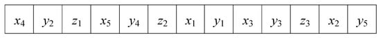
Figure 2. Individual coding mode.

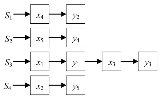
Figure 3. AGVs’ scheduling sequence.

2.2.2. Particle Fitness

The particle fitness is denoted by P. A penalty function is used to calculate P for searching for the problem’s optimal solution. We have:

$$P=\left\{\begin{array}{c}a\ast P_q+T , k=0\\ k\ast P_u ,k>0\end{array}\right.$$

(21)

where k represents the number of task points that do not conform to double-cycling, a represents the number of task points that do not conform to LTQ, P_q denotes a penalty coefficient for the LTQ, and P_u denotes a penalty coefficient for the double-cycling.

Particle fitness P includes 1) all AGVs’ waiting time and 2) the penalty value of task points in the scheduling sequence that do not conform to the LTQ. A solution may not meet the basic constraint of double-cycling, so before calculating P, the scheduling sequence should be judged whether it meets the basic constraint of double-cycling. If not, the particle fitness P is adjusted to the k ∗ P_u. The smaller the particle fitness, the better the scheduling sequence. We present an algorithm to solve the double-cycling model based on the HPSO algorithm in Algorithm 1. A flow chart of the algorithm is shown in Figure 4.

Algorithm 1 AGV double-cycling algorithm

Procedure HPSO

Input: Unloading task point set X, loading task point set Y, AGV number l, population size q, maximum iteration number tmax, the LTQ penalty coefficient Pq, the double-cycling penalty coefficient is Pu, particle fitness P, personal best position pBest, and global best particle gBest.

Output:gBest

for each particle i

Randomly Initialize a coding scheme Si for particle i

Calculate the fitness of particle i and set pBesti = Si

end for

gBest = min {pBesti}

while t < tmax

for I = 1 to q

Perform individual crossover, global crossover, and mutation operations to update the coding scheme of particle i

Calculate the fitness of particle i

if fitness (Si) < fitness (pBesti)

pBesti = Si;

if fitness (pBesti) < fitness (gBest)

gBest = pBesti;

end for

t = t + 1;

end while

print gBest

end procedure

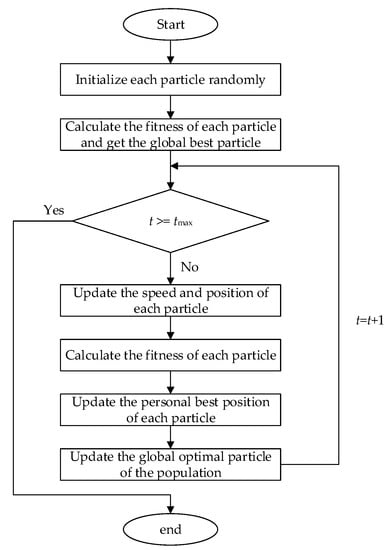
Figure 4. AGV double-cycling algorithm.

3. Results

Matlab_R2019a was used to solve the double-cycling model. First, we randomly generated a container scheduling sequence. In this work, a queue was formulated for each QC or YC. The task points were arranged in queues according to the container’s transportation order of the container scheduling sequence. The waiting time of the task points and the number of task points that did not meet the LTQ were calculated according to the relationship among the task points in the queue. Then, the scheduling sequence with the least number of task points that did not meet the LTQ and the least AGV waiting time were obtained using an HPSO algorithm. We then analyzed some critical parameters.

Corresponding waiting areas were set up at the quayside and the yard for storing AGVs that needed to wait. AGVs in the waiting area could turn off the engine or keep the engine on for waiting according to the estimated waiting time. The waiting time of the AGV that remained after starting the engine was a key to be considered in the double-cycling model. Table 5 show the data obtained in Qingdao Port from our field investigation.

Table 5. The data obtained in Qingdao Port.

Speed of QC	50 m/min
Speed of QC spreader	240 m/min
Grasping speed of QC spreader	180 m/min
Average time for QC to transport containers	60 s
Average travel time from the quayside to the yard	30 s
Speed of YC	270 m/min
Speed of YC spreader	180 m/min
Grasping speed of YC spreader	60 m/min
Average time for YC to transport containers	74 s
Speed of AGV	3 m/s
AGV travel time between two YCs	15 s
AGV travel time between two QCs	15 s

Table 6 show experimental results considering the total waiting time of the AGVs (Total Waiting Time), the number of task points that did not conform to LTQ (Not-Conform LTQ), the number of task points that did not conform to double-cycling (Not-Conform Double-cycling), and the fitness value.

Table 6. Results of multiple experiments in our double-cycle model.

Experiment Round	Not-Conform Doble-Cycling	Not-Conform LTQ	Fitness Value	Total Waiting Time (s)
1	0	0	944	944
2	0	0	1012	1012
3	0	0	939	939
4	0	0	941	941
5	0	0	965	965
6	0	0	1020	1020
7	0	0	1032	1032
8	0	0	1055	1055
9	0	0	960	960
10	0	0	1073	1073
11	0	1	1989	989
12	0	4	41,043	1043

First, a time disturbance that conformed to the Gaussian distribution was added to the QC operation time. We randomized the assignment according to the Gaussian distribution, so the results were not the same each time. In the double-cycling model, the experimental results showed that most scheduling sequences satisfy both double-cycling and LTQ. This work simulated the time disturbance existing in the QC operation, so a few experimental results failed to satisfy LTQ at all task points on the basic constraint of double-cycling. The number of task points that did not conform to LTQ was significantly higher in the last experiment than in other experiments. This situation was generally caused by the significant difference in the QC operation time in the last experiment and other experiments’ QC operation time, resulting in a severe phenomenon of AGV delays. The QC operator caused the time disturbance of QC operating time. Therefore, we think that the AGV could not reach the quayside in time due to the operator’s operation error. This part of the data should be discarded or recalculated. However, according to the experimental results in Table 6, there exists the phenomenon that some AGVs’ scheduling sequence was empty in the optimal scheduling sequence, which led to resource waste. To further improve the efficiency of the double-cycling system, this work continued to consider the influence of the number of AGVs on the efficiency of the double-cycling system. Table 7, Table 8, Table 9, Table 10 and Table 11 show the experimental results of changing the number of AGVs under a different number of task points on the base constraint of double-cycling, including the total waiting time of AGV and the number of task points that do not conform to LTQ. We selected three experimental results for each number of AGVs.

Table 7. The experimental results of different number of AGVs at 10 task points.

Number of AGVs	Number of Task Points	Experiment Round	Total Waiting Time (s)	Not-Conform LTQ
2	10	1	428	4
		2	496	4
		3	557	5
3	10	1	449	0
		2	405	0
		3	478	0
4	10	1	511	0
		2	481	0
		3	527	0

Table 8. The experimental results of different number of AGVs at 20 task points.

Number of AGVs	Number of Task Points	Experiment Round	Total Waiting Time (s)	Not-Conform LTQ
3	20	1	1122	4
		2	1110	6
		3	1086	5
4	20	1	1005	0
		2	1061	0
		3	1004	0
5	20	1	973	0
		2	929	0
		3	944	0
6	20	1	1086	0
		2	1112	0
		3	1061	0

Table 9. The experimental results of different number of AGVs at 30 task points.

Number of AGVs	Number of Task Points	Experiment Round	Total Waiting Time (s)	Not-Conform LTQ
4	30	1	2014	0
		2	2001	7
		3	1955	2
5	30	1	1903	0
		2	1890	0
		3	1910	0
6	30	1	1818	0
		2	1839	0
		3	1829	0
7	30	1	1847	0
		2	1861	4
		3	1823	0
8	30	1	1843	0
		2	1857	0
		3	1928	0

Table 10. The experimental results of different number of AGVs at 40 task points.

Number of AGVs	Number of Task Points	Experiment Round	Total Waiting Time (s)	Not-Conform LTQ
4	40	1	2689	0
		2	2721	5
		3	2717	1
5	40	1	2498	0
		2	2444	0
		3	2400	0
6	40	1	2679	0
		2	2687	0
		3	2624	0
7	40	1	2634	0
		2	2618	0
		3	2622	0
8	40	1	2584	0
		2	2653	0
		3	2678	0

Table 11. The experimental results of different number of AGVs at 50 task points.

Number of AGVs	Number of Task Points	Experiment Round	Total Waiting Time (s)	Not-Conform LTQ
5	50	1	3387	0
		2	3453	2
		3	3501	12
6	50	1	3398	0
		2	3296	0
		3	3438	2
7	50	1	3420	0
		2	3369	0
		3	3434	0
8	50	1	3333	0
		2	3308	0
		3	3610	0

For the different number of task points, we set different numbers of AGVs to transport them. The number of AGVs was gradually reduced until the constraint of conforming to LTQ could not be satisfied at all task points in most experiments, and the number of AGVs was set as the lower bound to transport the number of task points successfully. The number of AGVs was gradually increased until some AGVs’ scheduling sequence was still empty in most experiments, and the number of AGVs was set as the upper bound under the number of task points. Table 7, Table 8, Table 9, Table 10 and Table 11 show that for different numbers of task points, there was a corresponding number of AGVs to ensure that all task points met LTQ and had the minimum waiting time. For the number of task points in Table 7, Table 8, Table 9, Table 10 and Table 11, the appropriate AGVs were 3, 4, 5, 5, and 6, respectively. Too few AGVs will increase the number of task points that do not conform to LTQ, and too many AGVs will result in an increase in the waiting time of AGVs. Therefore, only an appropriate number of AGVs can improve the efficiency of the double-cycling model and make full use of transportation resources. In the real world, we can deal with containers on a ship layer by layer to break down a significant problem into more minor ones, and our model can then be applied. As mentioned above, the time disturbance of QC operation obeys different Gaussian distributions. This work discusses the influence of QC operations conforming to different Gaussian distribution models on the double-cycling system. Table 12 show the experimental results under different Gaussian distributions with 30 task points and five AGVs.

Table 12. The influence of QC conforms to different Gaussian distributions with 30 task points and 5 AGVs.

Experiment Round	$\mathit{\mu }=4, \mathit{\sigma }=4$		$\mathit{\mu }=4, \mathit{\sigma }=8$		$\mathit{\mu }=8, \mathit{\sigma }=8$		$\mathit{\mu }=8, \mathit{\sigma }=16$
	Total Waiting Time (s)	Not-Conform LTQ	Total Waiting Time (s)	Not-Conform LTQ	Total Waiting Time (s)	Not-Conform LTQ	Total Waiting Time (s)	Not-Conform LTQ
1	1813	0	1681	0	1871	0	2120	0
2	1797	0	1776	0	1845	0	2265	2
3	1695	0	1742	0	1876	0	1969	0
4	1782	0	1916	0	1947	0	2071	0
5	1861	0	1790	0	2067	2	1663	0
6	1882	0	1847	0	1914	0	1870	0
7	1831	0	1943	0	2221	0	2260	4
8	1849	0	1733	0	2020	4	1977	0
9	1812	0	1845	0	1851	0	2309	2
10	1821	0	1912	0	2019	0	1965	1

The smaller the μ and σ mean QC operator’s operation experience more affluent, and the smaller the time disturbance of the QC operation is. When μ = 4, σ = 4, the AGV’s waiting time fluctuates around 1814 s, with almost no QC delay. With the increase of μ and σ, the AGV waiting time fluctuates, and the QC delay becomes more and more frequent. The rise of σ leads to the increase of the time disturbance of QC operation, resulting in the AGV waiting time and the number of task points that do not conform to LTQ fluctuating significantly. The increase of μ postpones the time disturbance interval of QC operation, resulting in the AGV waiting time being longer. The experimental results show that the more experienced the QC operator is, the lower the AGV waiting time and QC delay times.

According to the model presented and relevant experimental results in this work, as long as the information of the task points set can be obtained, the iterative calculation of the task points set can be carried out in advance. The optimal container scheduling sequence is selected by adjusting the relevant factors, which proves the feasibility of the double-cycling model in practical situations. In the real world, we only need to consider the top layer of containers in the ship to break down the large problem into several small sub-problems. The sizes of the experiments conform to the real situation.

To ensure that the HPSO algorithm is excellent, the Simulated Annealing (SA) algorithm and Genetic Algorithm (GA) are designed for comparison in this work. It assumes that the success rate is S and the total number of experiments is E, where the number of successfully obtaining scheduling sequences that satisfy both LTQ and double-cycling constraints is e. The algorithm’s success rate is:

$$S=\frac{e}{E}\times 100\%$$

(22)

Table 13, Table 14 and Table 15 show that the three algorithms are compared with the success rate under the different number of task points and the success rate under the different numbers of μ and σ. Table 15 show the average execution time of the algorithm under the different number of task points.

Table 13. The success rate of the algorithm under different number of task points.

Number of Task Points	GA	HPSO	SA
12	90.19%	98.41%	88.23%
16	86.27%	98.33%	80.39%
20	84.31%	98.27%	75.55%
24	76.47%	96.07%	68.62%

Table 14. The success rate of the algorithm under different μ and σ.

(μ, σ)	GA	HPSO	SA
(4, 4)	88.46%	98.38%	87.23%
(4, 8)	86.27%	98.50%	85.10%
(8, 8)	82.35%	98.30%	82.22%
(8, 16)	78.43%	98.14%	74.5%

Table 15. The average execution time of the algorithm under different number of task points.

Number of Task Points	GA	HPSO	SA
12	25.96 s	12.85 s	32.76 s
16	28.87 s	14.82 s	41.13 s
20	42.65 s	17.12 s	69.50 s
24	65.42 s	18.24 s	113.38 s

Table 13 show that HPSO has the highest success rate in obtaining effective solutions. Table 14 show that HPSO has the most stable performance under different time disturbances. Table 15 show the HPSO algorithm takes the least time.

Meanwhile, Table 13, Table 14 and Table 15 show when the values of the μ and σ are small, the success rate is high. With the increase of the values of μ and σ, the algorithms’ success rate gradually declines, and the average execution time of the algorithms is more extended. Only the HPSO algorithm maintains a 90% success rate and a short average execution time. The reason for this result is the uncertainty of the QC operation. If the number of task points or the value of μ and σ increases, the transportation uncertainty on the quayside increases, resulting in an increasing number of task point sequences that cannot satisfy LTQ and double-cycling constraints.

4. Conclusions

To improve the utilization rate of AGVs in the process of CTs, this work proposes a double-cycling AGV scheduling model, which specifies that AGVs should enter and exit the yard and quayside with the full load during transportation. It reduces the empty running and minimizes the total waiting time of AGVs. The uncertainty of QC’s operation time is also considered. The container scheduling sequence is obtained by arranging the loading and unloading of containers based on the HPSO algorithm with a penalty function. The double-cycling mode can be adopted whenever containers need to be loaded and unloaded simultaneously. If the numbers of loading task points and unloading task points are not equal, we can choose some of the task points and use the double-cycling mode. We can adopt a multi-QC transportation mode for other complicated cases, and the QCs are divided into groups by the divide-and-conquer strategy. Each group has two quayside cranes for loading and unloading, respectively. The proposed model and algorithm are still key to realizing double cycling. More heuristic algorithms [37,38,39,40,41,42,43,44,45,46,47] will be used to solve the proposed problem in our future work.

References

- Saidi-Mehrabad, M.; Dehnavi-Arani, S.; Evazabadian, F.; Mahmoodian, V. An Ant Colony Algorithm (ACA) for solving the new integrated model of job shop scheduling and conflict-free routing of AGVs. Comput. Ind. Eng. 2015, 86, 2–13. [Google Scholar] [CrossRef]
- Angeloudis, P.; Bell, M.G.H. An uncertainty-aware AGV assignment algorithm for automated container terminals. Transp. Res. Part E Logist. Transp. Rev. 2010, 46, 354–366. [Google Scholar] [CrossRef]
- Luo, J.; Wan, Y.; Wu, W.; Li, Z. Optimal Petri-Net Controller for Avoiding Collisions in a Class of Automated Guided Vehicle Systems. IEEE Trans. Intell. Transp. Syst. 2020, 21, 4526–4537. [Google Scholar] [CrossRef]
- Ji, S.; Luan, D.; Chen, Z.; Guo, D. Integrated scheduling in automated container terminals considering AGV conflict-free routing. Transp. lett. 2020, 13, 510–513. [Google Scholar]
- Wang, Z.; Zeng, Q. A branch-and-bound approach for AGV dispatching and routing problems in automated container terminals. Comput. Ind. Eng. 2022, 166, 100968. [Google Scholar] [CrossRef]
- Zhong, M.; Yang, Y.; Dessouky, Y.; Postolache, O. Multi-AGV scheduling for conflict-free path planning in automated container terminals. Comput. Ind. Eng. 2020, 142, 106371. [Google Scholar] [CrossRef]
- Cavone, G.; Dotoli, M.; Seatzu, C. Resource planning of intermodal terminals using timed Petri nets. In Proceedings of the 2016 13th International Workshop on Discrete Event Systems (WODES), Xi’an, China, 30 May–1 June 2016; pp. 44–50. [Google Scholar]
- Rashidi, H.; Tsang, E.P.K. A complete and an incomplete algorithm for automated guided vehicle scheduling in container terminals. Comput. Math. Appl. 2011, 61, 630–641. [Google Scholar] [CrossRef]
- Hu, X.; Guo, J.; Zhang, Y. Optimal strategies for the yard truck scheduling in container terminal with the consideration of container clusters. Comput. Ind. Eng. 2019, 137, 106083. [Google Scholar] [CrossRef]
- Niu, B.; Zhang, F.; Li, L.; Wu, L. Particle swarm optimization for yard truck scheduling in container terminal with a cooperative strategy. Intell. Evol. Syst. 2017, 8, 333–346. [Google Scholar]
- Huang, S.Y.; Li, Y. A Bounded Two-Level Dynamic Programming Algorithm for Quay Crane Scheduling in Container Terminals. Comput. Ind. Eng. 2018, 123, 303–313. [Google Scholar] [CrossRef]
- Ji, M.; Guo, W.; Zhu, H.; Yang, Y. Optimization of loading sequence and rehandling strategy for multi-quay crane operations in container terminals. Transp. Res. Part E Logist. Transp. Rev. 2015, 80, 1–19. [Google Scholar] [CrossRef]
- Zhang, H.; Kim, K.H. Maximizing the number of dual-cycle operations of quay cranes in container terminals. Comput. Ind. Eng. 2009, 56, 979–992. [Google Scholar] [CrossRef]
- Nguyen, V.D.; Kim, K.H. Heuristic Algorithms for Constructing Transporter Pools in Container Terminals. IEEE Trans. Intell. Transp. Syst. 2012, 14, 517–526. [Google Scholar] [CrossRef]
- Zhen, L.; Yu, S.; Wang, S.; Sun, Z. Scheduling quay cranes and yard trucks for unloading operations in container ports. Ann. Oper. Res. 2019, 273, 455–478. [Google Scholar]
- Zhang, Z.; Liu, M.; Lee, C.; Wang, J. The Quay Crane Scheduling Problem with Stability Constraints. IEEE Trans. Autom. Sci. Eng. 2018, 15, 1399–1412. [Google Scholar] [CrossRef]
- Zhen, L. Container yard template planning under uncertain maritime market. Transp. Res. Part E Logist. Transp. Rev. 2014, 69, 199–217. [Google Scholar] [CrossRef]
- Sheikholeslami, A.; Ilati, R. A sample average approximation approach to the berth allocation problem with uncertain tides. Eng. Optim. 2018, 50, 1772–1788. [Google Scholar] [CrossRef]
- Wang, W.; Wu, Y. Is uncertainty always bad for the performance of transportation systems? Commun. Transp. Res. 2021, 1, 100021. [Google Scholar]
- Zheng, F.; Man, X.; Chu, F.; Liu, M.; Chu, C. A two-stage stochastic programming for single yard crane scheduling with uncertain release times of retrieval tasks. Int. J. Prod. Econ. 2019, 57, 4132–4147. [Google Scholar] [CrossRef]
- Ng, W.C.; Mak, K.L. Yard crane scheduling in port container terminals. Appl. Math. Model. 2005, 29, 263–276. [Google Scholar] [CrossRef] [Green Version]
- Javanshir, H.; Ghomi, S.M.T.F.; Ghomi, M.F. Investigating transportation system in container terminals and developing a yard crane scheduling model. Manag. Sci. Lett. 2012, 2, 171–180. [Google Scholar] [CrossRef]
- Diabat, A.; Theodorou, E. An Integrated Quay Crane Assignment and Scheduling Problem. Comput. Ind. Eng. 2014, 73, 115–123. [Google Scholar] [CrossRef]
- He, J.; Tana, C.; Zhang, Y. Yard crane scheduling problem in a container terminal considering risk caused by uncertainty. Adv. Eng. Inform. 2019, 39, 14–24. [Google Scholar] [CrossRef]
- Luo, J.; Wu, Y. Modelling of dual-cycle strategy for container storage and vehicle scheduling problems at automated container terminals. Transp. Res. Part E Logist. Transp. Rev. 2015, 79, 49–64. [Google Scholar] [CrossRef]
- Zheng, F.; Pang, Y.; Liu, M.; Xu, Y. Dynamic programming algorithms for the general quay crane double-cycling problem with internal-reshuffles. J. Comb. Optim. 2020, 39, 708–724. [Google Scholar] [CrossRef]
- Cao, J.X.; Shang, X.; Yao, X. Integrated quay crane and yard truck schedule for the dual-cycling strategies. In Proceedings of the CICTP 2017: Transportation Reform and Change—Equity, Inclusiveness, Sharing, and Innovation, Shanghai, China, 7–9 July 2017; pp. 1346–1357. [Google Scholar]
- Liu, M.; Chu, F.; Zhang, Z.; Chu, C. A polynomial-time heuristic for the quay crane double cycling problem with internal-reshuffling operations. Transp. Res. Part E Logist. Transp. Rev. 2015, 81, 52–74. [Google Scholar] [CrossRef]
- Wang, D.; Li, X. Quay crane scheduling with dual cycling. Engineering Optimization. Eng. Optim. 2015, 47, 1343–1360. [Google Scholar] [CrossRef]
- Nguyen, V.D.; Kim, K.H. Minimizing empty trips of yard trucks in container terminals by dual cycle operations. Ind. Eng. Manag. Syst. 2010, 9, 28–40. [Google Scholar] [CrossRef]
- Meisel, F.; Wichmann, M. Container sequencing for quay cranes with internal reshuffles. OR Spectr. 2010, 32, 569–591. [Google Scholar] [CrossRef]
- Goodchild, A.V.; Daganzo, C.F. Double-cycling strategies for container ships and their effect on ship loading and unloading operations. Transp. Sci. 2016, 40, 473–483. [Google Scholar] [CrossRef]
- Ahmed, E.; El-Abbasy, M.S.; Zayed, T.; Alfalah, G.; Alkass, S. Synchronized scheduling model for container terminals using simulated double-cycling strategy. Comput. Ind. Eng. 2021, 154, 107118. [Google Scholar] [CrossRef]
- Nishimura, E. Yard and berth planning efficiency with estimated handling time. Marit. Bus. Rev. 2020, 5, 5–29. [Google Scholar] [CrossRef] [Green Version]
- Guo, X.; Huang, S.Y.; Hsu, W.J.; Low, M.Y.H. Yard crane dispatching based on real time data driven simulation for container terminals. In Proceedings of the 2008 Winter Simulation Conference, Winter Simulation Conference, Miami, FL, USA, 7–10 December 2008; pp. 2648–2655. [Google Scholar]
- Kennedy, J.; Eberhart, R. Particle Swarm Optimization. In Proceedings of the ICNN’95—International Conference on Neural Networks, Perth, Australia, 27 November–1 December 1995; Volume 4, pp. 1942–1948. [Google Scholar]
- Guo, X.; Zhang, Z.; Qi, L.; Liu, S.; Tang, Y.; Zhao, Z. Stochastic Hybrid Discrete Grey Wolf Optimizer for Multi-objective Disassembly Sequencing and Line Balancing Planning in Disassembling Multiple Products. IEEE Trans. Autom. Sci. Eng. 2021, 1–3. [Google Scholar] [CrossRef]
- Guo, X.; Zhou, M.; Alsokhiry, F.; Sedraoui, K. Disassembly sequence planning: A survey. IEEE/CAA J. Autom. Sin. 2021, 8, 1308–1324. [Google Scholar] [CrossRef]
- Guo, X.; Zhou, M.; Liu, S.; Qi, L. Multi-resource Constrained Selective Disassembly with Maximal Profit and Minimal Energy Consumption. IEEE Trans. Autom. Sci. Eng. 2021, 18, 804–816. [Google Scholar] [CrossRef]
- Guo, X.; Zhou, M.; Liu, S.; Qi, L. Lexicographic Multiobjective Scatter Search for the Optimization of Sequence-Dependent Selective Disassembly Subject to Multiresource Constraints. IEEE Trans. Cybern. 2020, 50, 3307–3317. [Google Scholar] [CrossRef]
- Guo, X.; Liu, S.; Zhou, M.; Tian, G. Dual-objective program and scatter search for the optimization of disassembly sequences subject to multi-resource constraints. IEEE Trans. Autom. Sci. Eng. 2018, 15, 1091–1103. [Google Scholar] [CrossRef]
- Guo, X.; Liu, S.; Zhou, M.; Qi, L. Disassembly sequence optimization for large-scale products with multiresource constraints using scatter search and Petri nets. IEEE Trans. Cybern. 2016, 46, 2435–2446. [Google Scholar] [CrossRef]
- Zhao, Z.; Liu, S.; Zhou, M.; Guo, X.; Qi, L. Decomposition method for new single-machine scheduling problems from steel production systems. IEEE Trans. Autom. Sci. Eng. 2020, 17, 1376–1387. [Google Scholar] [CrossRef]
- Zhao, J.; Liu, S.; Zhou, M.; Guo, X.; Qi, L. Modified cuckoo search algorithm to solve economic power dispatch optimization problems. IEEE/CAA J. Autom. Sin. 2018, 5, 794–806. [Google Scholar] [CrossRef]
- Wang, X.; Zhou, M.; Zhao, Q.; Liu, S.; Guo, X.; Qi, L. A Branch and Price Algorithm for Crane Assignment and Scheduling in Slab Yard. IEEE Trans. Autom. Sci. Eng. 2021, 18, 1122–1133. [Google Scholar] [CrossRef]
- Zhao, Z.; Zhou, H.; Qi, L.; Chang, L.; Zhou, M. Inductive Representation Learning via CNN for Partially-Unseen Attributed Networks. IEEE Trans. Netw. Sci. Eng. 2021, 8, 695–706. [Google Scholar] [CrossRef]
- Ji, S.; Zhang, Q.; Li, J.; Chiu, D.K.W.; Xu, S.; Yi, L.; Gong, M. A burst-based unsupervised method for detecting review spammer groups. Inf. Sci. 2020, 536, 454–469. [Google Scholar] [CrossRef]
Publisher’s Note: MDPI stays neutral with regard to jurisdictional claims in published maps and institutional affiliations. |
© 2022 by the authors. Licensee MDPI, Basel, Switzerland. This article is an open access article distributed under the terms and conditions of the Creative Commons Attribution (CC BY) license (https://creativecommons.org/licenses/by/4.0/).