A Novel Anti-Jamming Technique for INS/GNSS Integration Based on Black Box Variational Inference

Abstract

In this paper, a novel anti-jamming technique based on black box variational inference for INS/GNSS integration with time-varying measurement noise covariance matrices is presented. We proved that the time-varying measurement noise is more similar to the Gaussian distribution with time-varying mean value than to the Inv-Gamma or Inv-Wishart distribution found by Kullback–Leibler divergence. Therefore, we assumed the prior distribution of measurement noise covariance matrices as Gaussian, and calculated the Gaussian parameters by the black box variational inference method. Finally, we obtained the measurement noise covariance matrices by using the Gaussian parameters. The experimental results illustrate that the proposed algorithm performs better in resisting time-varying measurement noise than the existing Variational Bayesian adaptive filter.

1. Introduction

The loosely integrated inertial navigation system (INS) and global navigation satellite system (GNSS) corrects INS errors and helps INS to complete navigation tasks by providing the velocity and position of the GNSS. However, GNSS signals are extremely weak when they reach the ground, hence, the signals are vulnerable to interference [1] such as radio signals that fall into the navigation signal pass band and multipath interference caused by reflection, scattering [2] or obstruction from buildings, tunnels and trees [3]. All of these interferences can lead to unknown noise statistics in GNSS navigation parameters. Thus, GNSS is unable to output accurate navigation information and eventually the INS/GNSS integration is unable to work properly.

The results of interference on GNSS parameters can be divided into three categories according to various studies. The first is GNSS outages. Because the GNSS cannot output navigation parameters, it is unable to complete auxiliary tasks [4]. Researchers usually solve such cases of interference by machine learning methods, such as neural network [5], regression algorithm [6], fault detection and isolation [7] or multiple receivers [8]. The second result is outliers in the GNSS navigation parameters [9]. For this type of interference, researchers usually set up the Student’s model to solve these issues [10]. The third outcome is that the navigation accuracy of the GNSS is lower than the accuracy without interference, but it can still complete auxiliary tasks, for example, the time-varying noise caused by interference. In this paper, the third type of interference noise will be researched.

The adaptive Kalman filter (AKF) is the most common method to solve the problem of time-varying noise [11]. The Sage–Husa AKF estimates the noise statistics recursively based on the maximum a posterior criterion [12,13]. However, the measurement noise of the actual system may be too small compared with the theoretical value, or the initial state noise setting might be too large, which results in the measurement noise covariance matrix (MNCM) losing its positivity and causes filtering divergence. Li et al. presented a multiple model AKF (MMAKF), which can deal with the model uncertainty by operating a bank of Kalman filters with different models simultaneously [14]. However, the MMAKF suffers from substantial computational complexities, and thus, MMAKF has poor real-time performance. Simo et al. first proposed the variational Bayesian (VB) AKF (VBAKF) model to solve the time-varying noise problem [15]. The VBAKF algorithm iteratively estimates the MNCM by using the variational inference (VI) method. The VBAKF algorithm is currently favored by many scholars because of its low computation requirements and accurate estimation. Li et al. applied VBAKF in target tracking to achieve accurate estimation of targets [16]. Shen et al. used VBAKF in INS/GNSS integration to estimate unknown MNCM [17]. Yu et al. proposed a series of VB nonlinear filtering for unknown MNCM, such as the VB Extended Kalman Filter (VBEKF), VB Untraced Kalman Filter (VBUKF), etc. [18]. The VB Cubature Kalman Filter (VBCKF) method was proposed to improve the estimation accuracy of nonlinear systems in [19]. VB and Monte Carlo sampling were used to solve the unknown measurement noise and uncertain parameters in [20]. Huang et al. solved the problem of inaccurate measurement noise and process noise with VBAKF [11]. However, Xu et al. proposed that the distribution of the process noise covariance matrix (PNCM) and the distribution of system state are non-conjugate, which cannot be solved directly by VBAKF. Therefore, they solved the inaccurate PNCM by black box variational inference (BBVI) [21].

In the existing anti-jamming methods based on VBAKF, to satisfy the conjugate conditions of the VBAKF algorithm, the prior distribution of MNCM was assumed to be an Inv-Gamma distribution or Inv-Wishart distribution. However, in the trial data of INS/GNSS integration, it was found that the time-varying noise was more similar to the Gaussian distribution with a changeable mean value. Therefore, in order to ensure the assumed approximate distribution was closer to the real distribution and estimate the MNCM more accurately, the Gaussian distribution was proposed as the prior distribution of MNCM in this paper. However, this assumption leads to a non-conjugate problem between the prior distribution and likelihood distribution. For this reason, the VBAKF algorithm cannot be used to estimate MNCM.

We learnt from [21], which used BBVI to solve the non-conjugate problem between the PNCM distribution and system state distribution. In this paper, a novel anti-jamming technique for INS/GNSS integration based on black box variational inference was proposed. We assumed the prior distribution of the MNCM was a Gaussian distribution. Then, we estimated the gradient of the Gaussian distribution parameters by using the BBVI algorithm. Lastly, we calculated the MNCM by using the parameters. The proposed algorithm and existing VBAKF were applied to the problem of INS/GNSS integration with time-varying measurement noise. Experimental results show that the proposed filter has a smaller root mean square error (RMSE) than existing VBAKF methods.

The remainder of the paper is organized as follows. First, we analyze the problems of VBAKF estimates of MNCM in the INS/GNSS integration. Second, the novel anti-jamming algorithm for INS/GNSS integration is presented. Third, the experimental results are analyzed and discussed. Finally, the conclusions are presented.

2. Problem Description

In this section, first, we establish the system models of INS/GNSS integration. Then, the influence of time-varying noise on the system is analyzed, and the VBAKF estimation method of MNCM is introduced. Finally, we analyze the distribution type of time-varying noise and the problems related to the existing VBAKF algorithm.

2.1. INS/GNSS Integration System Model

The loosely integrated INS/GNSS navigation system can output information on velocity, position, and attitude with the measurement information for velocity and position. The system models as follows.

As the application background in this paper is vehicle navigation, the navigation parameters of the horizontal are required to be higher. So, for the velocity and position parameters, we only take their horizontal parameters to establish the state equations. We take the errors of horizontal velocity, horizontal position, platform angles, accelerometer bias, and gyroscope bias as the state vectors [22], which can be written as

$$\mathit{X}=(\begin{array}{ccccccc}\delta v_{\mathrm{E}}& \delta v_{\mathrm{N}}& \delta \phi & \delta \lambda & {\varphi }_{\mathrm{E}}& {\varphi }_{\mathrm{N}}& {\varphi }_{\mathrm{U}}\end{array} {\begin{array}{cccccc}{\nabla }_{\mathrm{x}}& {\nabla }_{\mathrm{y}}& {\nabla }_{\mathrm{z}}& {\epsilon }_{\mathrm{x}}& {\epsilon }_{\mathrm{y}}& {\epsilon }_{\mathrm{z}}\end{array})}^{\mathrm{T}}$$

where $\mathit{X}$ is the state vector, $\delta v_{\mathrm{E}}$ and $\delta v_{\mathrm{N}}$ are the horizontal velocity errors, $\delta \phi$ and $\delta \lambda$ are the horizontal position errors, ${\varphi }_{\mathrm{E}}$, ${\varphi }_{\mathrm{N}}$, and ${\varphi }_{\mathrm{U}}$ are the misalignment angles, ${\nabla }_{\mathrm{x}}$, ${\nabla }_{\mathrm{y}}$, and ${\nabla }_{\mathrm{z}}$ are the accelerometer bias, ${\epsilon }_{\mathrm{x}}$, ${\epsilon }_{\mathrm{y}}$, and ${\epsilon }_{\mathrm{z}}$ are the gyroscope bias.

The measurement vectors derived from the difference between the velocity and position from the INS and GNSS can be given by

$$\mathit{Z}={\left(\begin{array}{cc}{\mathit{V}}_{\mathrm{INS}}-{\mathit{V}}_{\mathrm{GNSS}}& {\mathit{P}}_{\mathrm{INS}}-{\mathit{P}}_{\mathrm{GNSS}}\end{array}\right)}^{\mathrm{T}}$$

where $\mathit{Z}$ is the measurement vector, ${\mathit{V}}_{\mathrm{INS}}$ and ${\mathit{V}}_{\mathrm{GNSS}}$ are the horizontal velocity of INS and GNSS, respectively, and ${\mathit{P}}_{\mathrm{INS}}$ and ${\mathit{P}}_{\mathrm{GNSS}}$ are the horizontal position of INS and GNSS, respectively.

The state equations and measurement equations of the system are established based on the navigation coordinate system. The system models can be described as

$$\{\begin{array}{l}\dot{\mathit{X}}=\mathit{\Phi }\mathit{X}+\mathit{W}\\ \mathit{Z}=\mathit{H}\mathit{X}+\mathit{V}\end{array}$$

(1)

where Φ is the one-step state transition matrix, W is system noise, $\mathit{H}=\left[\begin{array}{cc}{\mathit{I}}_{4\times 4}& {{\displaystyle \mathit{0}}}_{4\times 9}\end{array}\right]$ is the measurement matrix. $\mathit{V}={\left[\begin{array}{cccc}{n}_{V_E}& n_{V_N}& n_{\phi }& n_{\lambda }\end{array}\right]}^{\mathrm{T}}$ is the measurement noise.

The state equations of Equation (1) are described in detail as follows.

$$\{\begin{array}{ll}\delta {\dot{V}}_E=& \delta V_E\frac{V_N\tan \phi }{R_N}+\delta V_N(2{\omega }_{ie}\sin \phi +\frac{V_E\tan \phi }{R_N})+\\ & \delta \phi (2{\omega }_{ie}{V}_N\cos \phi +\frac{V_E{V}_N}{R_N}{\sec }^2\phi )+{\varphi }_U{f}_N-{\varphi }_N{f}_U+{\nabla }_E^n\\ \delta {\dot{V}}_N=& -\delta V_E(2{\omega }_{ie}\sin \phi +\frac{2V_E\tan \phi }{R_N})-\\ & \delta \phi (2{\omega }_{ie}{V}_E\cos \phi +\frac{V_E{V}_E}{R_N}{\sec }^2\phi )-{\varphi }_U{f}_E+{\varphi }_E{f}_U+{\nabla }_N^n\\ \delta \dot{\phi }=& \frac{\delta V_N}{R_M}\\ \delta \dot{\lambda }=& \frac{\delta V_E}{R_N}\sec \phi +\delta \phi \frac{V_E}{R_N}\tan \phi \sec \phi \\ {\dot{\varphi }}_E=& -\frac{1}{R_M}\delta V_N+{\varphi }_N({\omega }_{ie}\sin \phi +\frac{V_E\tan \phi }{R_N})-{\varphi }_U({\omega }_{ie}\cos \phi +\frac{V_E}{R_N})+{\epsilon }_E^n\\ {\dot{\varphi }}_N=& -\frac{1}{R_N}\delta V_E-\delta \phi {\omega }_{ie}\sin \phi -{\varphi }_E({\omega }_{ie}\sin \phi +\frac{V_E\tan \phi }{R_N})-{\varphi }_U\frac{V_N}{R_M}+{\epsilon }_N^n\\ {\dot{\varphi }}_U=& \frac{\tan \phi }{R_N}\delta V_E+\delta \phi ({\omega }_{ie}\cos \phi +\frac{V_E}{R_N}{\sec }^2\phi )+{\varphi }_E({\omega }_{ie}\cos \phi +\frac{V_E}{R_N})+{\varphi }_N\frac{V_N}{R_M}+{\epsilon }_U^n\\ \dot{\mathit{\nabla }}=& 0\\ \dot{\mathit{\epsilon }}=& 0\end{array}$$

(2)

where $\left[\begin{array}{cc}{V}_E& V_N\end{array}\right]$ are the horizontal velocities, $\left[\begin{array}{cc}\phi & \lambda \end{array}\right]$ are the horizontal positions, ${\omega }_{ie}$ is the angular rate of the earth’s rotation, $R_M$ and $R_N$ are the earth radius, $\left[\begin{array}{ccc}{f}_E& f_N& f_U\end{array}\right]$ are the specific force.

In order to clearly describe the effect of time-varying noise on INS/GNSS integration, we conducted a simulation experiment. INS/GNSS integration operates without interference for 10 min. Then, the standard deviation of random white noise at the GNSS east and north position was increased from 5 m to 50 m. The standard deviation of random white noise at the east and north velocity was increased from 0.2 m/s to 2 m/s. The interference lasted for 5 min and then returned to the non-interference state. The total time of the simulation was 30 min. The influence of the time-varying noise on the velocity and position errors are shown in Figure 1 and Figure 2.

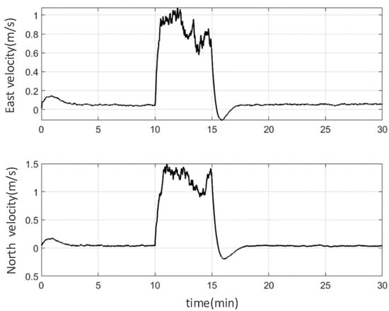
Figure 1. The influence of the time-varying noise on the velocity errors.

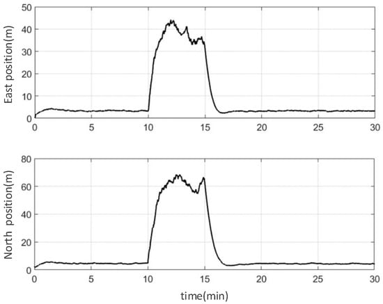
Figure 2. The influence of the time-varying noise on the position errors.

As demonstrated in Figure 1 and Figure 2, the velocity and position have large unsteady errors when time-varying noise appears in the measurement information. Therefore, it is necessary to estimate the accurate value of the MNCM to suppress the interference caused by time-varying noise to the navigation system.

2.2. Estimating MNCM with VBAKF

The statistical characteristics of V will be changed when GNSS is disturbed. Consequently, the MNCM is uncertain. At this point, if we continue to use the MNCM of the initial setting, the estimated values of the navigation parameters are not accurate. Therefore, MNCM should be estimated accurately to improve navigation accuracy.

The idea of estimating MNCM by VBAKF can be summarized as follows. First, the real distribution of MNCM is replaced with an approximate distribution. Then, Kullback–Leibler divergence (KLD) is used to measure the degree of similarity between the approximate distribution and the real distribution. When the evidence lower bound (ELB) reaches the maximum value, the KLD value is zero. That is, the approximate distribution is equal to the real distribution. Thus, the problem of estimating MNCM turns into the problem of solving the maximum value of ELB. The ELB maximum value can be solved by the VB general formula. However, the condition for using the VB general formula to solve the ELB maximum value is that the approximate distribution and likelihood distributions must be conjugate.

The steps for estimating time-varying MNCM by VBAKF are as follows.

In the framework of the Kalman filter, the likelihood distribution $p\left({\mathit{Z}}_k|{\mathit{R}}_k\right)$ is a Gaussian distribution, i.e.,

$$p\left({\mathit{Z}}_k|{\mathit{R}}_k\right)=\mathrm{N}\left({\mathit{Z}}_k;{\mathit{H}}_k{\mathit{X}}_k,{\mathit{R}}_k\right)$$

(3)

where $\mathit{R}$ is the MNCM. $\mathrm{N}\left(\cdot ;\ast ,\ast \right)$ denote the Gaussian probability density function (PDF).

In order to satisfy the conjugate condition, the prior distribution of MNCM $p\left({\mathit{R}}_k|{\mathit{Z}}_{1:k-1}\right)$ is assumed to be an Inv-Gamma distribution or Inv-Wishart distribution. We take the Inv-Gamma distribution, for example. It can be described as

$$p\left({\mathit{R}}_k|{\mathit{Z}}_{1:k-1}\right)={\displaystyle \prod _{i=1}^d\text{Inv-Gamma}\left({\mathit{R}}_{k,i};{\widehat{\mathit{\alpha }}}_{k|k-1,i},{\widehat{\mathit{\beta }}}_{k|k-1,i}\right)}$$

(4)

where d is the dimensions of R. $\mathit{\alpha }$ and $\mathit{\beta }$ are the parameters of the Inv-Gamma distribution. $\text{Inv-Gamma}\left(\cdot ;\ast ,\ast \right)$ denotes the Inv-Gamma PDF.

After the kth observation, we will replace $p\left({\mathit{R}}_k|{\mathit{Z}}_{1:k}\right)$ with a new approximate distribution $q\left({\mathit{R}}_k|{\mathit{Z}}_{1:k}\right)$. For simplicity, we omit the statement that the parameter R_k is dependent on Z_1:k in the approximate distribution. Thus, the new approximate distribution can be expressed as $q\left({\mathit{R}}_k\right)$.

According to the VB general formula, and taking the log of both sides of the general formula, we can obtain the ELB, which can be expressed as

$$\begin{array}{ll}\ln q\left({\mathit{R}}_k\right)& =\mathrm{E}\left[\ln p\left({\mathit{R}}_k|{\mathit{Z}}_{1:k-1}\right)\right]+\mathit{C}\\ & ={\displaystyle \sum _{i=1}^d\left[\left(-{\mathit{\alpha }}_{k|k-1,i}-\frac{1}{2}-1\right)\ln {\mathit{R}}_{k,i}^2\right]}-{\displaystyle \sum _{i=1}^d\frac{1}{{\mathit{R}}_{k,i}}\left[{\mathit{\beta }}_{k|k-1,i}+\frac{1}{2}\mathrm{E}\left[{\left({\left({\mathit{Z}}_k-{\mathit{H}}_k{\mathit{X}}_k\right)}_i\right)}^2\right]\right]}+\mathit{C}\end{array}$$

(5)

where C is the constants.

The VB general formula used in (5) can be described as

$$q\left({\theta }_i\right)=\frac{\exp \left({\mathrm{E}}_{q\left({\theta }_{k\ne i}\right)}\left[\left(\ln p\left(y,\theta \right)\right)\right]\right)}{{\displaystyle \int \exp \left({\mathrm{E}}_{q\left({\theta }_{k\ne i}\right)}\left[\ln p\left(y,\theta \right)\right]\right)} \mathrm{d}{\theta }_k}$$

(6)

where E[∙] denotes the expectation of $q\left({\theta }_i\right)$.

According to (5) and the logarithm of the Inv-Gamma PDF, we can see that R_k still obeys the Inv-Gamma distribution, which can be described as

$$q\left({\mathit{R}}_k\right)={\displaystyle \prod _{i=1}^d\text{Inv-Gamma}\left({\mathit{R}}_{k,i};{\widehat{\mathit{\alpha }}}_{k,i},{\widehat{\mathit{\beta }}}_{k,i}\right)}$$

(7)

According to the characteristics of the Inv-Gamma PDF, the expressions of the parameters are given by

$${\mathit{\alpha }}_{k,i}={\mathit{\alpha }}_{k|k-1,i}+\frac{1}{2}$$

(8)

$${\mathit{\beta }}_{k,i}={\mathit{\beta }}_{k|k-1,i}+\frac{1}{2}\mathrm{E}\left[{\left({\left({\mathit{Z}}_k-{\mathit{H}}_k{\mathit{X}}_k\right)}_i\right)}^2\right]$$

(9)

with

$$\mathrm{E}\left[{\left({\left({\mathit{Z}}_k-{\mathit{H}}_k{\mathit{X}}_k\right)}_i\right)}^2\right]={\left({\left({\mathrm{Z}}_k-{\mathit{H}}_k{\mathit{X}}_{k|k-1}\right)}_i\right)}^2+{\mathit{H}}_k{p}_k{\mathit{H}}_k^{\mathrm{T}}$$

(10)

where P is the predicted error covariance matrix.

According to the characteristics of the Inv-Gamma distribution, the MNCM estimation can be expressed as

$${\widehat{\mathit{R}}}_{k,i}=\mathrm{E}\left[{\mathit{R}}_{k,i}\right]={\mathit{\beta }}_{k,i}/{\mathit{\alpha }}_{k,i}$$

(11)

2.3. Measurement Noise Analyses

The distribution of the time-varying noise caused by GNSS signals interference is most similar to Gaussian distribution with a time-varying mean value. However, Inv-Gamma distribution or Inv-Wishart distribution is assumed as the prior distribution of the MNCM, when estimating the MNCM by VBAKF algorithm. All of this is to ensure the prior distribution and the likelihood distribution conjugate. Therefore, it will affect the estimation accuracy of the MNCM.

In order to prove the correctness of the above discussion, KLD was used to calculate the degree of similarity between time-varying noise and each distribution. We took a piece of trial data from the GNSS as an example. The time-varying noise of the GNSS east position is shown in Figure 3, where the data is derived from near the Airport Road. The distribution of the MNCM of the east position is shown in Figure 4. The Gaussian, Inv-Gamma, and Inv-Wishart distributions are shown in Figure 5.

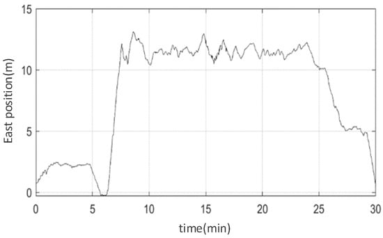
Figure 3. The time-varying noise of the GNSS east position.

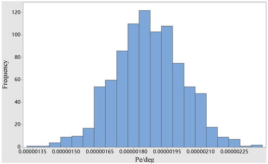
Figure 4. The distribution of GNSS east position noise.

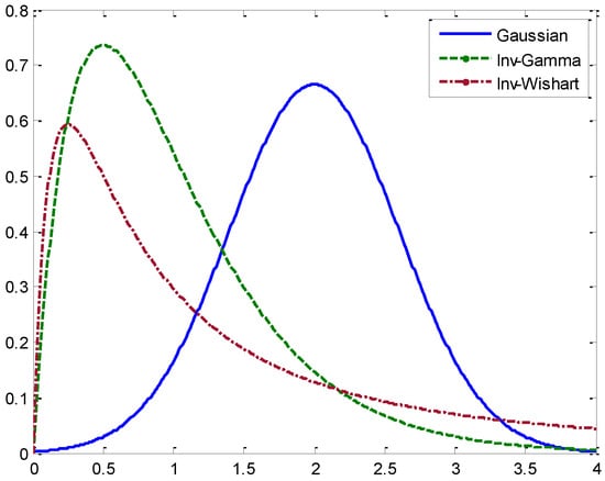
Figure 5. The Gaussian, Inv-Gamma, and Inv-Wishart distributions.

From Figure 4 and Figure 5, we can see that the time-varying noise still conforms to the Gaussian distribution, it is just that the mean value has changed. However, the distribution of time-varying noise is not similar to the Inv-Gamma and Inv-Wishart distributions. Next, we analyze the similarity between the noise distribution and each approximate distribution based on KLD.

The KLD formula is as follows

$$KL\left(p\left(x_i\right)\left|\right|q\left(x_i\right)\right)={\displaystyle \sum _{i=1}^{N}p\left(x_i\right)·\log \frac{p\left(x_i\right)}{q\left(x_i\right)}}$$

(12)

where $p\left(x_i\right)$ denotes the distribution of the GNSS east position time-varying noise. $q\left(x_i\right)$ denote the Gaussian, Inv-Gamma, or Inv-Wishart distribution. N is the number of samples.

According to (12), we can obtain the average Kullback–Leibler divergence (AKLD), which be defined as

$$\mathrm{AKL}\left(p\left(x_i\right)\left|\right|q\left(x_i\right)\right)=\frac{1}{M}{\displaystyle \sum _{m=1}^M{\mathrm{KL}}_m\left(p\left(x_i\right)\left|\right|q\left(x_i\right)\right)}$$

(13)

where M = 500 denote the numbers of experiment.

The AKLD values for each distribution and time-varying noise are shown in Table 1.

Table 1. The AKLD values.

Distribution	Gaussian	Inv-Gamma	Inv-Wishart
AKLD	1.557984	2.913936	2.639924

It can be seen from Table 1 that the Gaussian distribution is more similar to the distribution of the time-varying noise. However, the Inv-Gamma and Inv-Wishart distribution have poor similarity with the time-varying noise distribution.

3. The Novel Anti-Jamming Technique

In this section, first, the prior distribution of MNCM is assumed to be a Gaussian distribution, and the problems of the VBAKF algorithm are analyzed according to this assumption. Second, on the basis of the above analysis, we propose estimating the MNCM and completing the anti-jamming task of INS/GNSS integration by using the BBVI algorithm.

3.1. Prior Distribution of MNCM

The proofs in Section 2.3 show that the time-varying noise is closer to the Gaussian distribution. Therefore, we assume the prior distribution of the MNCM as Gaussian distribution. The prior distribution can be described as

$$p\left({\mathit{R}}_k|{\mathit{Z}}_{1:k-1}\right)=N\left({\mathit{R}}_k;{\widehat{\mathit{\mu }}}_{k|k-1},{\widehat{\mathit{\sigma }}}_{k|k-1}\right)$$

(14)

where $\mathit{\mu }$ and $\mathit{\sigma }$ are the expectation and variance of the R, respectively.

After the kth observation, we replace $p\left({\mathit{R}}_k|{\mathit{Z}}_{1:k-1}\right)$ with $q\left({\mathit{R}}_k|{\mathit{Z}}_{1:k}\right)$. According to general Formula (6), and taking the log of both sides of (6), the expression can be written as

$$\begin{array}{ll}\ln q\left({\mathit{R}}_k\right)& =\mathrm{E}\left[\ln p\left({\mathit{R}}_k|{\mathit{Z}}_{1:k-1}\right)\right]+\mathit{C}\\ & =-\frac{1}{2}[{\left({\mathit{R}}_k-{\widehat{\mathit{\mu }}}_{k|k-1}\right)}^{\mathrm{T}}{\mathit{\sigma }}^{-1}\left({\mathit{R}}_k-{\hat{\mathit{\mu }}}_{k|k-1}\right)]-\\ & \frac{1}{2}{\mathit{R}}_k{}^{-1}{\mathrm{E}}_{{\mathit{X}}_k}\left[{\left({\left({\mathit{Z}}_{1:k-1}-{\mathit{H}}_k{\mathit{X}}_k\right)}_i\right)}^2\right]-\frac{1}{2}\ln \left({\mathit{R}}_k{\widehat{\mathit{\sigma }}}_{k|k-1}\right)+\mathit{C}\end{array}$$

(15)

By comparing the logarithmic expression of the Gaussian PDF, from (15) it can be seen that the posterior distribution of MNCM no longer obeys the Gaussian distribution. That is, the prior distribution and the likelihood distribution are non-conjugate. Therefore, the conditions for VBAKF are not satisfied. The ELB cannot be calculated by the VI method, and the MNCM cannot be estimated.

Fortunately, Rajesh Ranganath et al. proposed the BBVI method, which aims to optimize the ELB by stochastic optimization. The condition for the approximate distribution and likelihood distribution to be conjugate is not required. More specifically, first, we form the derivative of the objective as an expectation with respect to the variational approximation; second, sampling from the variational approximation is used to get noisy but unbiased gradients; and last, we use the gradients to update the parameters of the approximate distribution [23].

3.2. BBVI Filter Based on Gaussian Distribution

By referencing the BBVI idea in [23] and the BBAKF method in [21], we derived the BBVI filter (BBVIF) anti-jamming algorithm with Gaussian distribution.

As in Section 3.1, we assume that the prior distribution of MNCM is a Gaussian distribution. The expression is the same as (14). After the kth observation, the gradients of ELB with respect to parameters can be expressed as

$${\mathit{\nabla }}_{\mathit{\lambda }}\mathit{ℒ}\left(\mathit{\lambda }\right)=E_{q\left({\mathit{R}}_k\right)}[{\mathit{\nabla }}_{\mathit{\lambda }}\log q\left({\mathit{R}}_k\right)\times \left(\log p\left({\mathit{Z}}_k,{\mathit{R}}_k|{\mathit{Z}}_{1:k-1}\right)-\log q\left({\mathit{R}}_k\right)\right)]$$

(16)

where $\mathit{\lambda }=\left\{\mathit{\mu },\mathit{\sigma }\right\}$ denotes the parameters of R. ${\mathit{\nabla }}_{\mathit{\lambda }}\mathit{ℒ}\left(\mathit{\lambda }\right)$ denotes the gradient of $\mathit{\lambda }$.

The ${\mathit{\nabla }}_{\mathit{\lambda }}\mathit{ℒ}\left(\mathit{\lambda }\right)$ can be approximated by a stochastic gradient estimator ${\widehat{\mathit{\nabla }}}_{\mathit{\lambda }}\mathit{ℒ}\left(\mathit{\lambda }\right)$ with Monte Carlo samples from variational distribution [21]. ${\widehat{\mathit{\nabla }}}_{\mathit{\lambda }}\mathit{ℒ}\left(\mathit{\lambda }\right)$ can be described as

$${\widehat{\mathit{\nabla }}}_{\mathit{\lambda }}\mathit{ℒ}\left(\mathit{\lambda }\right)\triangleq \frac{1}{S}{\displaystyle \sum _{S=1}^S\left[{\mathit{\nabla }}_{\mathit{\lambda }}\log q\left({\mathit{R}}_{k,S}\right)\times \left(\log p\left({\mathit{Z}}_{k,S},{\mathit{R}}_{k,S}|{\mathit{Z}}_{1:k-1,S}\right)-\log q\left({\mathit{R}}_{k,S}\right)\right)\right]}$$

(17)

where S is the number of samples.

With (17), we can use stochastic optimization to optimize the ELB of ${\mathit{\mu }}_k$ and ${\mathit{\sigma }}_k$. The expression can be written as

$${\widehat{\mathit{\nabla }}}_{{\mathit{\mu }}_k}\mathit{ℒ}\left({\mathit{\mu }}_k,{\mathit{\sigma }}_k\right)\triangleq \frac{1}{S}{\displaystyle \sum _{S=1}^S\left[{\mathit{\nabla }}_{{\mathit{\mu }}_k}\log q\left({\mathit{R}}_{k,S}\right)\times \left(\log p\left({\mathit{Z}}_{k,S},{\mathit{R}}_{k,S}|{\mathit{Z}}_{1:k-1,S}\right)-\log q\left({\mathit{R}}_{k,S}\right)\right)\right]}$$

(18)

$${\widehat{\mathit{\nabla }}}_{{\mathit{\sigma }}_k}\mathit{ℒ}\left({\mathit{\mu }}_k,{\mathit{\sigma }}_k\right)\triangleq \frac{1}{S}{\displaystyle \sum _{S=1}^S\left[{\mathit{\nabla }}_{{\mathit{\sigma }}_k}\log q\left({\mathit{R}}_{k,S}\right)\times \left(\log p\left({\mathit{Z}}_{k,S},{\mathit{R}}_{k,S}|{\mathit{Z}}_{1:k-1,S}\right)-\log q\left({\mathit{R}}_{k,S}\right)\right)\right]}$$

(19)

where the $\log p\left({\mathit{Z}}_{k,S},{\mathit{R}}_{k,S}|{\mathit{Z}}_{1:k-1,S}\right)$ is given by

$$\begin{array}{ll}\log p\left({\mathit{Z}}_{k,S},{\mathit{R}}_{k,S}|{\mathit{Z}}_{1:k-1,S}\right)& =\log \left[p\left({\mathit{Z}}_{k,S}|{\mathit{R}}_{k,S}\right)\cdot p\left({\mathit{R}}_{k,S}|{\mathit{Z}}_{1:k-1,S}\right)\right]\\ & =\log p\left({\mathit{Z}}_{k,S}|{\mathit{R}}_{k,S},{\mathit{Z}}_{1:k-1,S}\right)+\log p\left({\mathit{R}}_{k,S}|{\mathit{Z}}_{1:k-1,S}\right)\end{array}$$

(20)

with

$$\log q\left({\mathit{R}}_{k,S}\right)=\ln \frac{1}{2\pi }-\frac{1}{2}\ln {\mathit{\sigma }}_{k|k-1,S}-\frac{1}{2}\left({\mathit{R}}_{k,S}-{\mathit{\mu }}_{k|k-1,S}\right){\mathit{\sigma }}_{k|k-1}^{-1}\left({\mathit{R}}_{k,S}-{\mathit{\mu }}_{k|k-1,S}\right)$$

(21)

$${\mathit{\nabla }}_{{\mathit{\mu }}_k}\log q\left({\mathit{R}}_{k,S}\right)={\mathit{\sigma }}_{k|k-1,S}^{-1}\left({\mathit{R}}_{k,S}-{\mathit{\mu }}_{k|k-1,S}\right)$$

(22)

$${\mathit{\nabla }}_{{\mathit{\sigma }}_k}\log q\left({\mathit{R}}_{k,S}\right)=-\frac{1}{2}{\mathit{\sigma }}_{k|k-1,S}^{-1}+\frac{1}{2}{\mathit{\sigma }}_{k|k-1,S}^{-2}{\left({\mathit{R}}_{k,S}-{\mathit{\mu }}_{k|k-1,S}\right)}^2$$

(23)

According to [21], we updated the parameters of ${\mathit{\mu }}_k$ and ${\mathit{\sigma }}_k$ by stochastic optimization. The iterative method is as follows

$${\widehat{\mathit{\mu }}}_{k|k,i}={\widehat{\mathit{\mu }}}_{k|k-1,i}+\frac{\eta }{\sqrt{{\mathit{g}}_{k,i}+\epsilon }}{\widehat{\mathit{\nabla }}}_{{\mathit{\mu }}_{k,i}}\mathit{ℒ}\left({\mathit{\mu }}_{k,i},{\mathit{\sigma }}_{k,i}\right)$$

(24)

$${\widehat{\mathit{\sigma }}}_{k|k,i}={\widehat{\mathit{\sigma }}}_{k|k-1,i}+\frac{\eta }{\sqrt{{\mathit{G}}_{k,i}+\epsilon }}{\widehat{\mathit{\nabla }}}_{{\mathit{\sigma }}_{k,i}}\mathit{ℒ}\left({\mathit{\mu }}_{k,i},{\mathit{\sigma }}_{k,i}\right)$$

(25)

where g_k and G_k are updated by the Adaptive Gradient (AdaGard), the expressions are given by

$${\mathit{g}}_k=\gamma {\mathit{g}}_{k-1}+\left(1-\gamma \right){\widehat{\mathit{\nabla }}}_{{\mathit{\mu }}_k}{\mathit{ℒ}}^2\left({\mathit{\mu }}_k,{\mathit{\sigma }}_k\right)$$

(26)

$${\mathit{G}}_k=\gamma {\mathit{G}}_{k-1}+\left(1-\gamma \right){\widehat{\mathit{\nabla }}}_{{\mathit{\sigma }}_k}{\mathit{ℒ}}^2\left({\mathit{\mu }}_k,{\mathit{\sigma }}_k\right)$$

(27)

The variance in the estimator of the gradient (under the Monte Carlo estimate in Equation 16) may be too large to be useful when we use the method above to maximize the ELB. In practice, a higher variance gradient requires very small steps, which will lead to a slow convergence. Therefore, the variance needs to be reduced in the original method. Here, we refer to [23], and adopt the control variates method. The minimum variance is given by

$${\mathit{a}}_{{\mathit{\mu }}_k}=\frac{\mathrm{cov}\left({\mathit{f}}_s\left({\mathit{\mu }}_k\right),{\mathit{h}}_s\left({\mathit{\mu }}_k\right)\right)}{\mathrm{var}\left({\mathit{h}}_s\left({\mathit{\mu }}_k\right)\right)}$$

(28)

$${\mathit{A}}_{{\mathit{\sigma }}_k}=\frac{\mathrm{cov}\left({\mathit{F}}_s\left({\mathit{\sigma }}_k\right),{\mathit{H}}_s\left({\mathit{\sigma }}_k\right)\right)}{\mathrm{var}\left({\mathit{H}}_s\left({\mathit{\sigma }}_k\right)\right)}$$

(29)

with

$${\mathit{f}}_s\left({\mathit{\mu }}_k\right)={\mathit{\nabla }}_{{\mathit{\mu }}_k}\log q\left({\mathit{R}}_S\right)\times \left(\log p\left({\mathit{R}}_S,{\mathit{Z}}_{1:k,S}|{\mathit{Z}}_{1:k-1,S}\right)-\log q\left({\mathit{R}}_S\right)\right)$$

(30)

$${\mathit{h}}_s\left({\mathit{\mu }}_k\right)={\mathit{\nabla }}_{{\mathit{\mu }}_k}\log q\left({\mathit{R}}_S\right)$$

(31)

$${\mathit{F}}_s\left({\mathit{\sigma }}_k\right)={\mathit{\nabla }}_{{\mathit{\sigma }}_k}\log q\left({\mathit{R}}_S\right)\times \left(\log p\left({\mathit{R}}_S,{\mathit{Z}}_{1:k,S}|{\mathit{Z}}_{1:k-1,S}\right)-\log q\left({\mathit{R}}_S\right)\right)$$

(32)

$${\mathit{H}}_s\left({\mathit{\sigma }}_k\right)={\mathit{\nabla }}_{{\mathit{\sigma }}_k}\log q\left({\mathit{R}}_S\right)$$

(33)

With control variates, the new method to compute the gradients of ELB with respect to parameters can be expressed as

$${\widehat{\mathit{\nabla }}}_{{\mathit{\mu }}_k}{\mathit{ℒ}}_c\left({\mathit{\mu }}_k,{\mathit{\sigma }}_k\right)\approx \frac{1}{S}{\displaystyle \sum _{S=1}^S\left[{\mathit{f}}_s\left({\mathit{\mu }}_k\right)-{\mathit{a}}_{{\mathit{\mu }}_k}{\mathit{h}}_s\left({\mathit{\mu }}_k\right)\right]}$$

(34)

$${\widehat{\mathit{\nabla }}}_{{\mathit{\sigma }}_k}{\mathit{ℒ}}_c\left({\mathit{\mu }}_k,{\mathit{\sigma }}_k\right)\approx \frac{1}{S}{\displaystyle \sum _{S=1}^S\left[{\mathit{F}}_s\left({\mathit{\sigma }}_k\right)-A_{{\mathit{\sigma }}_k}{\mathit{H}}_s\left({\mathit{\sigma }}_k\right)\right]}$$

(35)

According to the characteristics of Gaussian distribution, the estimated value of the MNCM can be given by

$${\widehat{\mathit{R}}}_k=E\left[{\mathit{R}}_k\right]={\mathit{\mu }}_k$$

(36)

The procedure for the anti-jamming method based on BBVI is summarized in Algorithm 1.

Algorithm 1. Summary of the novel anti-jamming method for INS/GNSS integration based on BBVI.

Input: X0, Zk, P0, Q0, R0, µ0, σ0, g0, G0, ɛ0, η0, γ0.

Time update (the same as Kalman Filter)

1. ${\hat{\mathit{X}}}_{k|k-1}={\mathit{\Phi }}_{k|k-1}{\hat{\mathit{X}}}_{k-1}$

2. ${\mathit{P}}_{k|k-1}={\mathit{\Phi }}_{k|k-1}{\mathit{P}}_{k-1}{\mathit{\Phi }}_{k|k-1}^{\mathrm{T}}+{\mathit{Q}}_{k-1}$

Measurement update (BBVI method)

3. Draw S samples: ${\mathit{R}}_{k,S}\sim q\left({\mathit{R}}_{k,S}\right)$,

$q\left({\mathit{R}}_{k,S}\right)\sim \mathrm{N}\left({\mathit{R}}_{k,S};{\widehat{\mathit{\mu }}}_{k|k-1},{\widehat{\mathit{\sigma }}}_{k|k-1}\right)$

4. for S = 1 to S do

5. Update ${\mathit{f}}_s\left({\mathit{\mu }}_k\right)$ and ${\mathit{h}}_s\left({\mathit{\mu }}_k\right)$ as in (28) and (29).

6. Update ${\mathit{F}}_s\left({\mathit{\sigma }}_k\right)$ and ${\mathit{H}}_s\left({\mathit{\sigma }}_k\right)$ as in (30) and (31).

end for

7. Calculate ${\mathit{a}}_{{\mathit{\mu }}_k}$ and ${\mathit{A}}_{{\sigma }_k}$ as in (26) and (27).

8. Estimate the gradients ${\widehat{\mathit{\nabla }}}_{{\mathit{\mu }}_k}{\mathit{ℒ}}_c\left({\mathit{\mu }}_k,{\mathit{\sigma }}_k\right)$ and ${\widehat{\mathit{\nabla }}}_{{\mathit{\sigma }}_k}{\mathit{ℒ}}_c\left({\mathit{\mu }}_k,{\mathit{\sigma }}_k\right)$ as in (32) and (33).

9. Update ${\mathit{g}}_k$ and ${\mathit{G}}_k$ as in (24) and (25).

10. Update ${\widehat{\mathit{\mu }}}_{k|k}$ and ${\widehat{\mathit{\sigma }}}_{k|k}$ as in (22) and (23).

11. Calculate ${\widehat{\mathit{R}}}_k$ as in (35).

11. ${\mathit{K}}_k={\mathit{P}}_{k|k-1}{\mathit{H}}_k^{\mathrm{T}}{\left({\mathit{H}}_k{\mathit{P}}_{k|k-1}{\mathit{H}}_k^{\mathrm{T}}+{\widehat{\mathit{R}}}_k\right)}^{-1}$

12. ${\hat{\mathit{X}}}_k={\hat{\mathit{X}}}_{k|k-1}+{\mathit{K}}_k\left({\mathit{Z}}_k-{\mathit{H}}_k{\hat{\mathit{X}}}_{k|k-1}\right)$

13. ${\mathit{P}}_k=\left(\mathit{I}-{\mathit{K}}_k{\mathit{H}}_k\right){\mathit{P}}_{k|k-1}$

Output:${\hat{\mathit{X}}}_k$,${\mathit{P}}_k$.

To clearly demonstrate the difference between the VBAKF algorithm based on the Inv-Gamma or Inv-Wishart distribution and the proposed algorithm, the two algorithms are shown in Figure 6.

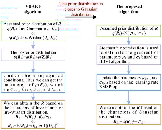
Figure 6. The algorithm flowchart of VBAKF and the proposed algorithm where l is the degrees of freedom parameter, and U is the inverse scale matrix.

As can be seen in Figure 6, in order to describe the prior distribution of the MNCM more accurately, the Gaussian distribution was selected as the approximate distribution of MNCM in this paper. Furthermore, in order to solve the problem that the prior distribution and likelihood distribution are non-conjugate after selecting the Gaussian distribution, and the problem that VBAKF cannot be applied, we proposed estimating the MNCM by the stochastic optimization of the BBVI algorithm.

4. Experimental Results and Analyses

In a previous study, the performance of the VBAKF was compared with the existing AKF in dealing with time-varying MNCM, and VBAKF proved to be superior to the existing AKF [11]. Therefore, we only compared the BBVI with the VBAKF algorithm, whose prior distribution is an approximate Inv-Gamma and Inv-Wishart distribution. Furthermore, the performance of the BBVIF anti-jamming algorithm with Gaussian distribution was verified by simulation and trial data.

4.1. Experiments with Simulation Data

The validity of the proposed algorithm was verified by simulations. The simulation conditions are set as follows.

The initial position is latitude 45.783898 degrees north and longitude 126.69458 degrees east. The Simulation lasts 60 min.

The specifications of the INS and GNSS are listed in Table 2.

Table 2. Specifications of the INS and GNSS.

INS		GNSS
Gyro bias	0.02°/h	Velocity	1 m/s
Accelerometer bias	5 mg	Position	8 m
Update rate	100 HZ	Update rate	1 HZ

Interference conditions are set as follows.

The ranges of interference: (20 min–25 min) and (40 min–45 min). Velocity error of GNSS: 3 m/s. Position error of GNSS: 15 m.

According to the above interference settings, the variation in GNSS velocities’ noise and position noise caused by interference are shown in Figure 7 and Figure 8.

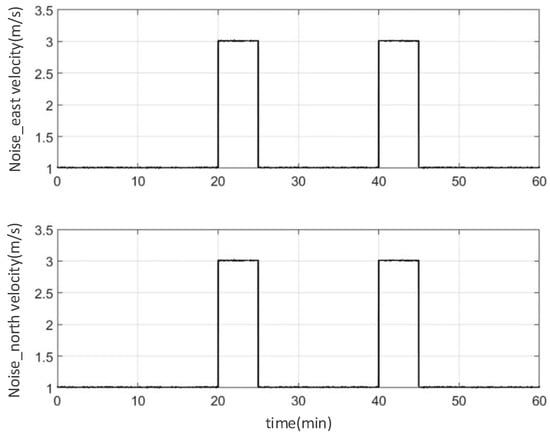
Figure 7. Variation in GNSS velocities’ noise.

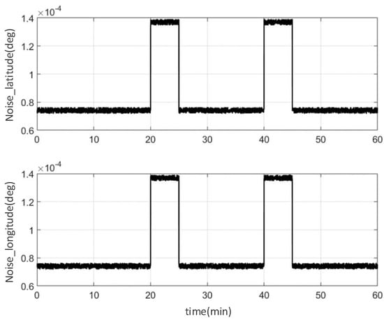
Figure 8. Variation in GNSS position’s noise.

To evaluate the accuracy of the methods, the RMSE of velocity and position were used as performance metrics. It was defined as

$$\mathrm{RMSE}\triangleq \frac{1}{M}{\displaystyle \sum _{l=1}^M\left(x_k^l-{\widehat{x}}_k^l\right)}$$

(37)

where $x_k^l$ denotes the true navigation parameters, and ${\widehat{x}}_k^l$ is the estimated navigation parameters. $M=500$ represents the total number of Mont Carlo runs.

A previous study proved the influence of different sample numbers on the BBVI method [21], and concluded that the algorithm has the fastest convergence speed when S = 50. Thus, S = 50 was selected as the sample number in this paper. In addition, the parameters of the proposed method were set as

$$\eta =10, \gamma =0.5, \mathit{g}=0, \mathit{G}=0, \epsilon =1\times {10}^{-10}.$$

Before the navigation parameters of each algorithm were shown, we used Inv-Gamma, Inv-Wishart and Gaussian prior models to estimate the MNCM values. We take the north velocity for example, and the estimated MNCM values and the true MNCM values of the north velocity are shown in the Figure 9.

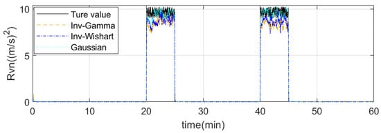
Figure 9. MNCM values of the north velocity. Rvn is the MNCM value of the north velocity.

For a clearer description of the estimated MNCM values, a larger version of Figure 10 is shown in Figure 9.

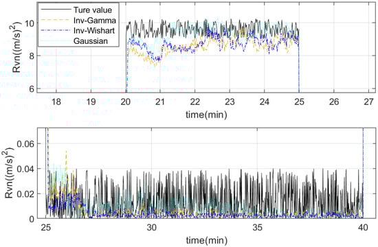
Figure 10. The enlarged figure of MNCM values.

It can be seen from Figure 9 and Figure 10 that all three models can estimate the MNCM values of north velocity. It shows that all three methods can play an anti-jamming role. However, the MNCM values estimated by Inv-Gamma and Inv-Wishart prior models were both smaller than the true MNCM values, and the MNCM estimated by the Gaussian prior model is more accurate than the other two models. This would lead to inaccurate estimation of navigation parameters by the Inv-Gamma or Inv-Wishart models. Therefore, the anti-jamming effect is not as good as the proposed algorithm.

We evaluated the anti-jamming effect of each algorithm from the estimated navigation parameters. The RMSEs of the velocity and position from the existing VBAKF and the proposed algorithm are shown in Figure 11 and Figure 12, respectively.

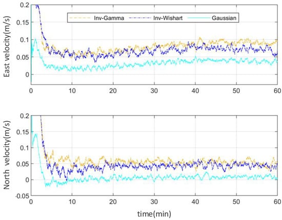
Figure 11. RMSEs of the velocity using the simulation data.

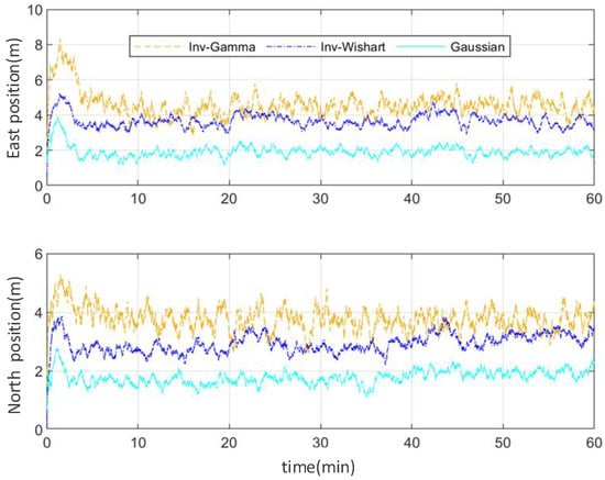
Figure 12. RMSEs of the position using the simulation data.

Table 3 shows the RMSEs of the velocity and position from existing VBAKF and the proposed algorithm, respectively.

Table 3. RMSEs of velocity and position using the simulation data.

Parameters	Gaussian	Inv-Gamma	Inv-Wishart
Ve (m/s)	0.0241	0.0873	0.0667
Vn (m/s)	0.0096	0.0627	0.0422
Pe (m)	1.8024	3.3576	2.9498
Pn (m)	2.0643	4.7653	3.6865

Figure 11 and Figure 12 and Table 3 show that the proposed algorithm with the prior Gaussian distribution has smaller RMSEs than the existing VBAKF algorithm with the prior distribution of Inv-Gamma or Inv-Wishart. The velocity and position accuracy of the proposed method is 3–4 times and 1–2 times higher than the existing VBAKF method, respectively. It also can be seen that the RMSEs of the velocity and position for the VBAKF based on the prior distribution of Inv-Gamma are similar to those estimated by the VBAKF based on the prior distribution of Inv-Wishart. The latter has a slightly higher accuracy compared with the former.

The simulation results and analyses proved that the prior distribution of MNCM is closer to the Gaussian distribution. Moreover, the correctness of the navigation parameters and effectiveness of the anti-jamming by the proposed algorithm were also proven.

4.2. Experiments with Trial Data

Simulation results showed the validity of the proposed method. Then, the feasibility and practicality of the proposed algorithm in engineering was verified by trial data.

The trial data was derived from near the Airport Road. The INS/GNSS integration system was composed of a laser inertial navigation system (LINS) and GNSS. The accuracy of the LINS is 1.5 n mile/h. The output rate is 400 HZ. The position and velocity accuracy of GNSS are 10 m and 5 m/s, respectively. The output rate is 1 HZ. The true value of the navigation parameters are given by the PHINS, which was provided by the IXSEA company. The experimental platform is shown in Figure 13.

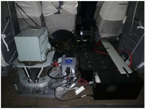
Figure 13. Experimental platform.

As the radio signals fall right into the navigation signal pass band or there is multipath interference caused by buildings, the noise of the GNSS navigation parameters is time-varying. The time-varying interference noise is shown in Figure 3.

The BBVIF anti-jamming algorithm with Gaussian distribution was compared with the VBAKF algorithm with Inv-Gamma or Inv-Wishart distribution by using the trial data. The RMSEs of the velocity and position are shown in Figure 14 and Figure 15 and Table 4. Furthermore, driving trajectories of the anti-jamming algorithms described above and the reference value provided by PHINS are shown in Figure 16. To see the driving trajectories more clearly, we have magnified a corner of the trajectories, and this is shown in the bottom right corner of Figure 16.

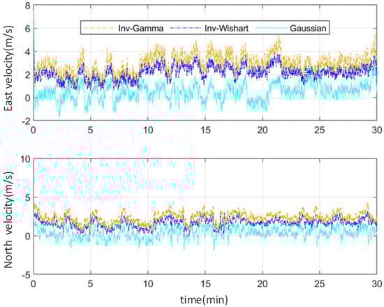
Figure 14. RMSEs of the velocity using the trial data.

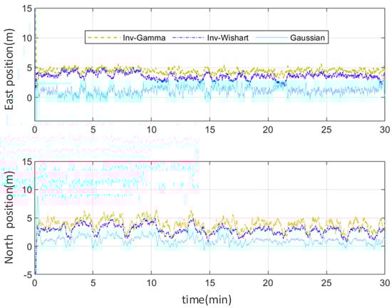
Figure 15. RMSEs of the position using the trial data.

Table 4. RMSEs of velocity and position using the trial data.

Parameters	Gaussian	Inv-Gamma	Inv-Wishart
Ve (m/s)	0.834	2.601	2.144
Vn (m/s)	0.603	2.268	1.789
Pe (m)	1.239	3.887	3.502
Pn (m)	1.089	3.592	3.342

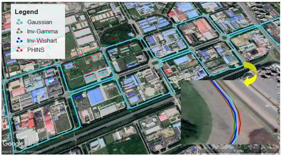
Figure 16. Driving trajectories near the Airport Road.

The results based on the trial data show that all three methods can complete the task of anti-jamming, which is the same as the simulations. The accuracy of the navigation parameters from the BBVIF with Gaussian distribution is higher than the VBAKF with Inv-Gamma or Inv-Wishart distribution. The velocity and position accuracy of the proposed method is approximately 3 times higher than the existing VBAKF method. It is because of the time-varying noise is more similar to Gaussian. Therefore, the BBVIF with Gaussian distribution estimate is more accurate than the other two algorithms. This experimental result proved that the proposed algorithm is feasible and practical in engineering applications.

5. Discussion

Here, we have presented a novel anti-jamming technique for integration based on BBVI. First, KLD was used to prove that compared with Inv-Gamma or Inv-Wishart distributions, the Gaussian distribution with time-varying mean value is closer to the time-varying noise. Accordingly, the prior distribution of the MNCM was assumed to be Gaussian. Second, to solve the problem that the VBAKF cannot be applied when the prior distribution and likelihood distribution are non-conjugate, we proposed the use of the BBVI method, which is based on stochastic optimization, instead of the VI method to estimate the time-varying MNCM. Finally, the validity and engineering practicality of the proposed method were verified by simulations and trial data. This novel anti-jamming algorithm, which deals with time-varying measurement noise provides more accurate estimation and stronger anti-jamming performance than previous methods. Significantly, compared with VBAKF, the algorithm in this paper improves the accuracy of estimation. However, the algorithm is more complex than VBAKF because it needs to calculate the gradient of ELBO and then update the parameters by stochastic optimization. This is where we need to improve in future work.

References

- Liu, Y. Study on Multidimensional Interference Suppression for Satellite Navigation System. Ph.D. Thesis, Beijing Institute of Technology, Beijing, China, 2016. [Google Scholar]
- Wu, Z.K.; Wang, W. INS/magnetometer integrated positioning based on neural network for bridging long-time GPS outages. GPS Solut. 2019, 23, 88. [Google Scholar] [CrossRef]
- Yang, L.; Li, Y.; Wu, Y. An enhanced MEMS-INS/GNSS integrated system with fault detection and exclusion capability for land vehicle navigation in urban areas. GPS Solut. 2014, 18, 293–294. [Google Scholar] [CrossRef]
- Sadra, R.; Hossein, N.; Jafar, K. Fuzzy-adaptive constrained data fusion algorithm for indirect centralized integrated SINS/GNSS navigation system. GPS Solut. 2019, 23, 62. [Google Scholar]
- Shen, C.; Zhang, Y.; Tang, J. Dual-optimization for a MEMS-INS/GPS system during GPS outages based on the cubature Kalman filter and neural networks. Mech. Syst. Signal Process. 2019, 133, 4–8. [Google Scholar] [CrossRef]
- Adusumilli, S.; Bhatt, D.; Wang, H.; Devabhaktuni, V.; Bhattacharya, P. A novel hybrid approach utilizing principal component regression and random forest regression to bridge the period of GPS outages. Neurocomputing 2015, 166, 185–192. [Google Scholar] [CrossRef]
- Zhong, L.; Liu, J.; Li, R. Approach for detecting soft faults in GPS/INS integrated navigation based on LS-SVM and AIME. J. Navig. 2017, 70, 561–579. [Google Scholar] [CrossRef]
- Liu, D.; Wang, H.J.; Xia, Q.Y.; Jiang, C.H. A Low-Cost Method of Improving the GNSS/SINS Integrated Navigation System Using Multiple Receivers. Electronics 2020, 9, 1079. [Google Scholar] [CrossRef]
- Wang, D.; Meng, D.; Li, Z.; Dong, Y.; Wu, J. Adaptively outlier-restrained GNSS/MEMS-INS integrated navigation method. Chin. J. Sci. Instrum. 2017, 38, 2954–2955. [Google Scholar]
- Huang, Y.L.; Zhang, Y.G. Robust Student’s t based stochastic cubature filter for nonlinear systems with heavy-tailed process and measurement noises. IEEE Access 2017, 5, 7966–7970. [Google Scholar] [CrossRef]
- Huang, Y.L.; Zhang, Y.G.; Wu, Z.M.; Li, N.; Jonathon, C. A Novel Adaptive Kalman Filter With Inaccurate Process and Measurement Noise Covariance Matrices. IEEE Trans. Autom. Control 2018, 63, 594–597. [Google Scholar] [CrossRef]
- Sage, A.; Husa, G. Adaptive filtering with unknown prior statistics. In Proceedings of the Joint Automatic Control Conference, Boulder, CO, USA, 5–7 August 1969. [Google Scholar]
- Gao, X.; You, D.; Katayama, S. Seam tracking monitoring based on adaptive Kalman filter embedded Elman neural network during high power fiber laser welding. IEEE Trans. Ind. Electron. 2012, 59, 4315–4324. [Google Scholar] [CrossRef]
- Li, X.; Bar-Shalom, Y. A recursive multiple model approach to noise identification. IEEE Trans. Aerosp. Electron. Syst. 1994, 30, 671–684. [Google Scholar] [CrossRef]
- Simo, S.; Aapo, N. Recursive Noise Adaptive Kalman Filtering by Variational Bayesian Approximations. IEEE Trans. Autom. Control 2009, 54, 596–600. [Google Scholar]
- Li, Z.; Zhang, J.; Wang, J.; Zhou, Q. Recursive Noise Adaptive Extended Object Tracking by Variational Bayesian Approximation. IEEE Access 2019, 7, 151168–151179. [Google Scholar] [CrossRef]
- Shen, C.; Xu, D.; Shen, F.; Cai, J. Variational bayesian adaptive Kalman filtering for GPS/INS integrated navigation. J. Harbin Inst. Technol. 2014, 46, 59–65. [Google Scholar]
- Yu, X.; Li, J.; Xu, J. Nonlinear filtering in unknown measurement noise and target tracking system by variational Bayesian inference. Aerosp. Sci. Technol. 2019, 84, 37–55. [Google Scholar] [CrossRef]
- Cui, B.; Wei, X.; Chen, X.; Li, J.; Wang, A. Robust cubature Kalman filter based on variational Bayesian and transformed posterior sigma points error. ISA Trans. 2019, 86, 18–28. [Google Scholar] [CrossRef] [PubMed]
- Yu, X.; Li, J.; Xu, J. Robust adaptive algorithm for nonlinear systems with unknown measurement noise and uncertain parameters by variational Bayesian inference. Int. J. Robust Nonlinear Control 2018, 28, 3475–3500. [Google Scholar] [CrossRef]
- Xu, H.; Duan, K.; Yuan, H.; Xie, W.; Wang, Y. Black box variational inference to adaptive kalman filter with unknown process noise covariance matrix. Signal Process. 2020, 169, 1–9. [Google Scholar] [CrossRef]
- Dong, P.; Cheng, J.H.; Liu, L.Q.; Sun, X.Y.; Fan, S.L. A Heading Angle Estimation Approach for MEMS-INS/GNSS Integration Based on ZHVC and SAUKF. IEEE Access 2019, 7, 154084–154095. [Google Scholar] [CrossRef]
- Ranganath, R.; Gerrish, S.; Blei, D. Black Box Variational Inference. In Proceedings of the International Conference on Artificial Intelligence and Statistics, Reykjavik, Iceland, 22–25 December 2013. [Google Scholar]
Publisher’s Note: MDPI stays neutral with regard to jurisdictional claims in published maps and institutional affiliations. |
© 2021 by the authors. Licensee MDPI, Basel, Switzerland. This article is an open access article distributed under the terms and conditions of the Creative Commons Attribution (CC BY) license (https://creativecommons.org/licenses/by/4.0/).