Abstract
This study constructs a nonlinear dynamic model of articulated vehicles and a model of hydraulic steering system. The equations of state required for nonlinear vehicle dynamics models, stability analysis models, and corresponding eigenvalue analysis are obtained by constructing Newtonian mechanical equilibrium equations. The objective and subjective causes of the snake oscillation and relevant indicators for evaluating snake instability are analysed using several vehicle state parameters. The influencing factors of vehicle stability and specific action mechanism of the corresponding factors are analysed by combining the eigenvalue method with multiple vehicle state parameters. The centre of mass position and hydraulic system have a more substantial influence on the stability of vehicles than the other parameters. Vehicles can be in a complex state of snaking and deviating. Different eigenvalues have varying effects on different forms of instability. The critical velocity of the linear stability analysis model obtained through the eigenvalue method is relatively lower than the critical velocity of the nonlinear model.
1. Introduction
Articulated vehicles with small steering radius and positive maneuverability are extensively used in mining, construction, forestry, emergency rescue, and other fields [1,2]. Articulated vehicles consist of two separate front and rear vehicles and an articulated steering device connecting the both vehicles. This particular form of construction and steering results in underdeveloped stability, specifically at high speed, and the snaking instability phenomenon will occur [1,3]. This situation increases the operating burden and danger for drivers and limits the speed and efficiency of articulated vehicles. Therefore, the factors influencing the stability and snaking instability of articulated vehicles should be studied.
Numerous studies examined the instability of articulated vehicles, and two research methods for the stability analysis of these vehicles are currently available. The first approach assumes that vehicles travel at a constant speed, obtains the corresponding characteristic equations by linearising the vehicle dynamics model and analyses the vehicle state using the eigenvalue method [4,5,6]. The other approach uses numerical integration methods to obtain responses to some arbitrary inputs [7,8]. The majority of the related studies have used the first method for the corresponding analysis of articulated vehicles. School and Klein [9] studied the steering system, simulation model and stability criteria to gain an improved understanding of the closed loop stability characteristics. Horton and Crolla [5,10] firstly invoked the eigenvalue method to judge the stability of articulated vehicles. Snaking critical velocity is obtained when the real part of the eigenvalue is positive. He analysed the correspondence between articulated vehicle jack-knife and snaking. Azad [4,11] provided an overview of lateral stability analysis. The influence of some vehicle structure parameters on the stability of articulated vehicles is analysed. Gao [12,13] studied the critical speed of articulated vehicles’ hydraulic steering systems with different hydraulic moduli of elasticity. Xu [3] studied the snaking mode under different conditions by the articulated angle. Dudziński and Skurjat [14] analysed the effects of air content in the fluid and vehicle drive form on the articulated angle. Eigenvalue analysis is limited to linear or linearised models and is considered valid near the point of linearization [15]. Rehnberg [6] built a scaled test vehicle model, and verified the practicality of the stability analysis method based on the linearised kinetic model. Stiffer steering leads to high frequency of snaking, and flexible suspension negatively affects snaking stability [16]. Liu [8] constructed a nonlinear vehicle dynamics model and used an integration method to derive an analytical periodic solution of the system in the neighborhood of the critical speed. Mu [17] showed that elastic torsional suspension can improve the roll stability of vehicles, but the directional stability at high speed of vehicles with suspension is poorer than that of vehicles without suspension. Lopatka and Muszynski [18] analysed the limited perception of driver, which has insensitivity zones of the lateral and angular locations. Drivers rely heavily on rotational motion and their senses to prevent vehicles from snaking; hence, drivers have a significant impact on vehicle stability.
The current study constructs a nonlinear articulated vehicle dynamics model and hydraulic steering system model. The nonlinear dynamics model, stability analysis models and equations of state are obtained using Newtonian mechanical equations relative to the previous generalised force approach, specifically by deriving the Lagrange equations. The characteristics of snaking are investigated, and the causes of snaking are analysed using multiple vehicle status parameters. The factors influencing the stability of articulated vehicles are analyzed, and the influence of some new factors are specifically studied. Vehicle instability can be in the snaking and deviating complex compound state. A better analysis of vehicle stability can be conducted by combining eigenvalue curves with vehicle status parameters compared with mere eigenvalue curves.
2. Modelling of Non-Linear Systems for Articulated Vehicles
Articulated vehicle structures are relatively complex, and different simplification methods for establishing articulated vehicle dynamics models can be broadly divided into two-dimensional planar models [10,19] and three-dimensional spatial models [20,21]. Two-dimensional planar models study the lateral, longitudinal and transverse motions of vehicles on a plane. Tire forces are obtained through the vertical distribution of gravity, axial load transfer and relevant experienced or semi-experienced tire models. Three-dimensional spatial models involve substantially complex effects, such as roll motion and suspension, and the models can directly calculate tire forces based on tire vertical displacement and associated tire models. The vehicle coordinate system can be divided into a one-coordinate [19,20] and two-coordinate [22,23] systems. The one-coordinate system often takes the articulated centre as the coordinate origin. The relevant research parameters can be obtained by dereferencing the excursions of the rotational inertia and dynamic balance equations of the front and rear vehicles. The two-coordinate system often considers the front and rear plasmas as the coordinate origin. The relevant research parameters are obtained through coordinate transformation or constructing kinematic relationships between the front and rear vehicles. One of the mathematical means for modelling global dynamics is to construct generalised coordinates and generalised forces, and derive the Lagrange equations [4,24]. The other method uses Newtonian mechanics to construct mechanical equilibrium equations. According to dissimilar research questions, the reasonable simplification of models and selection of appropriate modelling methods can improve efficiency and obtain superior results.
The vehicle dynamics model is the research foundation of vehicle handling and stability characteristics. However, owing to the special steering mechanism of articulated vehicles, front and rear vehicles coupling, non-linear influence of tires, axle load transfer and other factors, accurate articulated vehicle nonlinear system models should be established, including vehicle dynamics, tire and hydraulic steering models.
2.1. Vehicle Dynamics Analysis and Modelling
The articulated vehicle dynamics model is simplified as follows based on this study’s research objectives.
- (1)
- The front and rear body centres are located on the longitudinal central axis, and the vehicle is symmetrical with respect to the longitudinal central axis.
- (2)
- The influence of the tire camber angle and return torque on wheel dynamics are disregarded.
- (3)
- Air resistance is disregarded, and the road surface is flat and two-dimensional.
The articulated vehicle dynamics model is shown in Figure 1. The force analysis of the articulated vehicle is performed to obtain the equations of the equilibrium for the lateral, longitudinal and transverse swings of the front and rear vehicles.
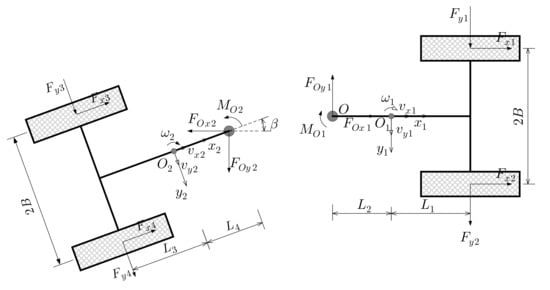
Figure 1.
Articulated vehicle dynamics model.
Based on the structural and kinematic relationship of the front and rear vehicles, the relationships between the front and rear vehicles are as follows:
An analysis of snaking indicates that articulated vehicles move in a straight line. Given that lateral and longitudinal accelerations cause axial load transfer, the transferred load should be distributed in addition to self-gravity. The articulated vehicle vertical force analysis is shown in Figure 2, and the vertical force of each tire is shown in Equation (7).
where , , , , , , , and .
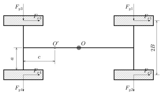
Figure 2.
Articulated vehicle vertical force analysis.
2.2. Tire Models
External forces on vehicles are mainly applied by the ground to the vehicle body through the tires. Thus, the tire model affects the vehicle dynamics, and is often a non-linear model. This study uses the Dugoff tire model, and the tire model is complementary to the elastic basis analysis model developed by Fiala and the lateral force-vertical force synthesis model of Pacejka and Sharp. The tire model provides a method to calculate forces under the combined lateral and longitudinal forces [18]. The most important feature is that it is fast and requires only a few parameters for calculation. The lateral and longitudinal forces of tires can be obtained according to the vertical force, tire sideslip angle and longitudinal slip rate. The model equations are as follows:
where , . Substituting Equations (7) to (12) in Equation (13) obtains the tire lateral and longitudinal forces for each wheel.
2.3. Hydraulic Steering System Model
The hydraulic steering system model has a significant impact on the stability of articulated vehicles. When articulated vehicles travel in a straight line or at a fixed radius, the inlet and outlet ports of the steering valve are closed, and the hydraulic steering system is equivalent to a torsion spring acting at the steering hinge point and connecting the front and rear bodies [12]. The hydraulic steering model is shown in Figure 3.
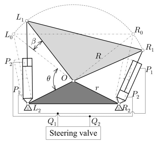
Figure 3.
Hydraulic steering system model.
The lengths of the left and right steering cylinders and the lengths of the two cylinders when are as follows:
The force arms corresponding to the thrust of the hydraulic cylinders on both sides are as follows:
where is the fluid volume of the chamber, is the volume of the fluid in the initial position, and are the cross-sectional area of the rod less and rod cavities, respectively, is the amount of oil supplied to the steering cylinder and is the amount of oil discharged from the steering cylinder.
When the articulated vehicle is travelling straight or at a fixed radius, :
The left and right hydraulic cylinder forces are as follows:
The hydraulic steering system has a torque on the articulation points of the articulated vehicles:
2.4. Model Simulation
On the basis of the nonlinear dynamics mathematical model of the previously described articulated vehicle, the articulated vehicle dynamics simulation model was built in the MATLAB/Simulink simulation environment. The simulation model includes the vehicle dynamics, tire, driver, hydraulic steering system and vertical force calculation models. The parameters in the model are shown in Table 1.

Table 1.
Parameters of the vehicle dynamics model.
To verify the snaking, the vehicle travels at an initial speed of (disregarding rolling friction) and exerts a pulse moment interference on the articulated points. The parameters of each vehicle are in a state of oscillatory convergence with decreasing amplitude, as shown in Figure 4. Owing to interference, the ground exerts lateral forces on the tires, thereby generating lateral and angular accelerations about the z-axis in different directions and amplitudes for the front and rear vehicles. The front and rear vehicles produce lateral and angular velocities about the z-axis, and the vehicle’s swing angle changes accordingly, thereby resulting in the snaking phenomenon. Owing to vehicle structural parameters, ground and speed, the swing angle is in a state of oscillatory convergence, while the snaking oscillation is in a steady state. Ideally, if the friction between the ground and tires is zero, then the entire snaking oscillation system of the vehicle is oscillating without damping, and the swing angle should be an equal amplitude oscillation. If the snaking is unstable under the influence of vehicle parameters, ground, speed and other factors, then the swing angle and corresponding parameters will oscillate and diverge.
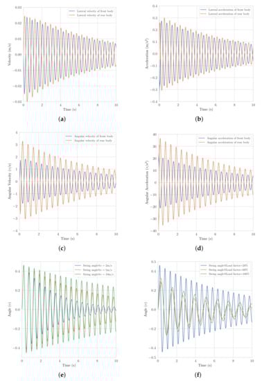
Figure 4.
Simulation results: (a) lateral velocity, (b) lateral acceleration, (c) angular velocity, (d) angular acceleration, (e) variation of the swing angle regarding the vehicle velocity, and (f) variation of the swing angle regarding the load factor.
Numerous reasons can be cited for snaking, the most important of which is the compressibility of the hydraulic fluid in the hydraulic steering system, thereby results in a certain degree of stiffness of the hydraulic steering system. Other vehicle parameters also affect the stability of vehicles, such as the position of the centre of gravity, tire stiffness, hydraulic system characteristics and other factors. Ideally, when the road is completely flat and in the same condition, the lateral and longitudinal forces on the ground are identical for each tire, thereby substantially producing snaking. However, the fact is that roads will not be in ideal condition, the forces acting on the wheels will be different and non-structural terrain will increase the occurrence of snaking. When drivers operate vehicles under the road surface or other external disturbance, they will have a poor driving experience and misuse the steering system to suppress the effect of the swing or deviation. However, this situation alters the steady state and increases snaking, thereby creating a vicious cycle.
To investigate the effects of velocity variation and different loads on the swing angle, several sets of simulations were performed. As shown in Figure 4e, the vehicles are all in steady state at three different velocities of 2 m/s, 5 m/s and 10 m/s. As the vehicle velocity increases, the convergence rate of the swing angle gradually decreases which means the vehicle stability tends to decrease as the velocity increases. The vehicles are also in steady state at three different loads of 20%, 60% and 100% load factor of the front vehicle, as shown in Figure 4f, the amplitude of the swing angle decreases with the increase of the load factor. The oscillation frequency of the swing angle is lower at high load factor area than that at low load factor area. Due to the influence of vehicle weight and the moment of inertia, the relationship between the swing angle and load factor is not linear. Overall, the increase in vehicle load factor is beneficial for vehicle stability.
The verification and analysis of the snaking phenomenon of the articulated vehicle dynamics model shows the reliability of the entire vehicle dynamics model. Accordingly, stability and snaking influence factor analyses can be performed.
3. Stability Analysis Model for Articulated Vehicles
On the basis of Lyapunov stability analysis theory, the eigenvalue method is used to analyse the relationship between vehicle parameters and stability. For the analysis, the kinetic model developed in the previous section is linearised. The forward velocity is assumed to be constant. In the event of snaking in articulated vehicles, the longitudinal force is relatively small compared with the lateral force. Hence, the longitudinal force can be disregarded. Moreover, the hydraulic steering system can be equivalent to a torsion spring, as shown in Figure 5. It should be noted that we have enlarged the articulated angle in the figure to facilitate interpretation, i.e., the actual is not as large as shown in the figure.
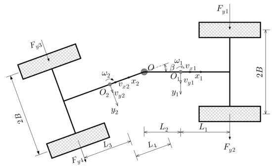
Figure 5.
Simplified model of vehicle dynamics.
The vehicle dynamics equation can be expressed as follows:
Since is considerably small that it is acceptable to assume , then the first equation in Equation (21) can be simplified to
The front and rear vehicle kinematics relationship is as follows:
Tire forces can be expressed as follows:
Hydraulic systems can be equated as follows:
In conjunction with Equations (21) to (24), the system dynamics differential equation group is obtained with the equation of state as follows:
where , , , , , , , , , , , , , , , .
According to the Lyapunov stability conditions, the stability of articulated vehicles is related to the real part of each eigenvalue of the equation of state. When the real part of each eigenvalue of the equation of state is negative/positive, the vehicles are in a stable/unstable state.
4. Analysis of the Stability Influencing Factors
4.1. Effects of the Centre of Mass Position
Owing to the wide range of engineering applications of articulated vehicles, different loads and working devices can change the position of the centre of mass. In changing the distance from the front and rear mass centre positions to the articulation point, stability analysis theory is used to study the effects of the centre of mass position. The distance between the front and rear mass centres was changed from , to , and , . The eigenvalues and swing angle are shown in Figure 6.
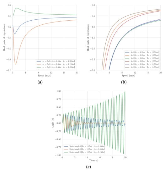
Figure 6.
Variation of the real parts of the eigenvalues and swing angle with the center of mass: (a) real parts of and , (b) real parts of and , and (c) swing angle of the vehicle.
When and , the real parts of the eigenvalues of and are positive, the corresponding oscillation of the swing angle is diverging, the swing angle is increasing and the vehicle is unstable. The other two conditions have negative eigenvalues, corresponding to the convergence of the swing angle, but the , corresponding eigenvalues are significantly smaller, and the swing angle converges rapidly. This result means that decreasing the distance between the centre of mass position and articulation point is beneficial for increasing vehicle stability. When the centre of mass position exceeds the position of the wheel axle, the parameter has a significant impact on the stability of vehicles (i.e., may cause instability). Therefore, when designing an articulated vehicle structure, the centre of mass should be positioned as far inside the wheel axle as possible, and the distance between the centre of mass position and articulation point should be as short as possible.
4.2. Effects of Torsional Stiffness
Engineering hydraulic oil modulus of elasticity can assume a fixed value, but leakage from hydraulic steering systems, a certain amount of air in the fluid, hydraulic pipes and other influencing factors, the hydraulic oil composite modulus of elasticity of the articulated vehicle steering system will be substantially reduced compared with the ideal situation. The stability of articulated vehicles under different elastic moduli of , , , , and the eigenvalues and swing angles are shown in Figure 7. The eigenvalues , are negative, while the two conditions with the lower modulus of elasticity at higher velocity of the eigenvalues , are positive. The analysis of the results indicate that the higher the hydraulic oil composite modulus of elasticity, the greater the rigidity of the hydraulic steering system, the more stable the vehicles and the faster the convergence of the swing angle. However, the amplitude of the swing angle is not linearly related to the elastic modulus, i.e., the higher the elastic modulus, the higher the oscillation frequency.
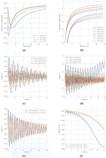
Figure 7.
Variation of the real parts of the eigenvalues, swing angles and lateral velocity with the torsional stiffness: (a) real parts of and , (b) real parts of and , (c) swing angle of the vehicle at , (d) swing angle of the vehicle at , (e) swing angle of the vehicle at critical velocity, and (f) lateral velocity.
Kinetic simulations of two lower elastic moduli at the respective critical velocities are performed separately, and the respective swing angles are in a steady state. When the velocity exceeds the critical speed of a certain range, the vehicle bending angle does not oscillate with equal amplitude in the centre of line zero, but gradually deviates from the state of the centre line of the oscillation with a type of amplitude gradually decreasing, and the lateral velocities of the vehicle gradually increase. At the time the vehicle is in a relatively deviating stage with snaking, the smaller the modulus of elasticity, the faster the deviation. The stability analysis model differs from vehicle nonlinear dynamics model owing to linearisation. According to the analytical curves, the critical velocity obtained by the linearised model is relatively lower than the critical velocity obtained by the nonlinear dynamics model.
4.3. Effects of Mass
Different loads on vehicles result in the front and rear masses being in a varying state. The stability characteristics of the front and rear vehicles under 1.5 times the original mass are studied, and the eigenvalues are shown in Figure 8. All eigenvalues are negative, the articulated vehicle is in a stable state and changing the mass will not have a substantial impact on stability in a certain range of vehicle parameters. According to the change in eigenvalue curves, increasing the mass of the front vehicle will increase the stability of the articulated vehicle, while increasing the mass of the rear vehicle will reduce the stability of the articulated vehicle volume.
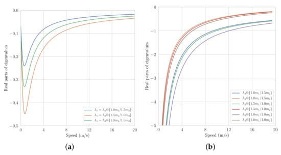
Figure 8.
Variation of the real parts of the eigenvalues with the vehicle mass: (a) real parts of and and (b) real parts of and .
4.4. Effects of the Moment of Inertia
The stability characteristics of the front and rear vehicles under 1.5 times the original rotational inertia are studied separately, and the eigenvalues are shown in Figure 9. All eigenvalues are negative and the articulated vehicle is in a stable state. Similar to the effects of mass, stable vehicle parameters indicate that changing the moment of inertia within a certain range will not have a significant effect on stability. According to the eigenvalue curves, increasing the moments of inertia of the front and rear vehicles increase and decrease, respectively, the stability of the articulated vehicle.
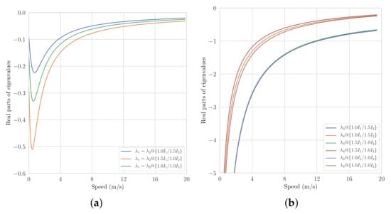
Figure 9.
Variation of the real parts of the eigenvalues with the moment of inertia: (a) real parts of and and (b) real parts of and .
4.5. Effects of Tire Cornering Stiffness
Tyres are the component of the vehicle that directly contacts the ground and their condition has a crucial impact on the stability of the vehicle. In addition, pressure is one of the key parameters of a tyre. It is difficult or even impossible to establish a universal model to accurately calculate the relationship between tire pressure and cornering stiffness for different tires. Several related studies [25] showed that the relationship between the cornering stiffness and the tire pressure is approximately linear under heavy load. As articulated vehicles are mostly heavy construction vehicles which means the tires are always under heavy load, so the cornering stiffness is very likely to increases as the tire pressure increase linearly. Therefore, the effect of tires pressure on stability can be analysed implicitly by analysing the effect of cornering stiffness on stability.
The stability characteristics of articulated vehicles under different tire cornering stiffness conditions are studied, and the values are shown in Figure 10. All eigenvalues are negative, and the articulated vehicle is in a stable state. According to the eigenvalue curve, increasing tire stiffness will increase the stability of the vehicle. Therefore, in terms of stability, tires with high rigidity should be chosen as much as possible when designing vehicle matching.
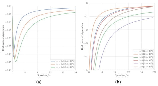
Figure 10.
Variation of the real parts of the eigenvalues with the tire stiffness: (a) real parts of and and (b) real parts of and .
4.6. Effects of the Hydraulic Cylinder Force Arm
The position of the hinge point of the hydraulic cylinder affects the stiffness of the hydraulic system and also has an impact on the stability of articulated vehicles. The stability characteristics of articulated vehicles with different force arms are studied, and the values are shown in Figure 11. and are negative, while and are positive at high velocity for the small force arms. The analysis of the results indicates that the larger the force arm, the more rigid the hydraulic steering system and the more stable the articulated vehicles. Moreover, articulated vehicles with small force arm will seemingly deviate with high speed, thereby indicating that the vehicle is in an unstable state. Therefore, the force arm should be designed as large as possible to increase the stability.
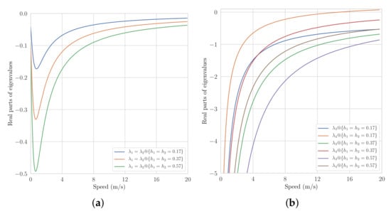
Figure 11.
Variation of the real parts of the eigenvalues with the hydraulic cylinder force arm: (a) real parts of and and (b) real parts of and .
5. Discussion
A nonlinear articulated vehicle dynamics model and hydraulic steering system model are established in this research. By studying the curve characteristics of the swing angle, lateral velocity, lateral acceleration and angular velocity and angular acceleration parameters in the snaking phenomenon, the evaluation and analysis indexes of the snaking are determined. The causes of the snaking phenomenon are analysed from the perspective of mechanical principles and subjective and objective factors (e.g., drivers and environment).
5.1. Conclusions
A linearised stability analysis model was established to analyse the factors influencing the stability of articulated vehicles. The centre of mass position, modulus of elasticity of the hydraulic fluid, tire stiffness, mass, rotational inertia and hydraulic cylinder arm have an impact on vehicle stability. An effective method for determining vehicle stability was established by combining eigenvalue curves with vehicle condition. Stability analysis indicates that the stability of articulated vehicles decreases with increasing speed regardless of the state of these vehicles. Among the vehicle parameters, centre of mass position and hydraulic system have a more substantial influence on the stability of articulated vehicles than the other parameters. The real parts of and have a substantial influence on snaking instability, while the real parts of and have a significantly deviating instability influence. Articulated vehicles are in unstable and compound state of snaking and deviating. The critical velocity obtained by the linearised model is relatively lower than the critical velocity obtained by the nonlinear dynamics model. The eigenvalue curve can be used to identify and compare the state of vehicles. An effective stability analysis method is formed to provide the basis for vehicle structural design and vehicle parameter matching and control methods in optimising vehicle stability.
5.2. Limitation and Outlook
Owing to several limitations, no experiments were carried out in this paper. Considering the safety factor, in the subsequent research, this study will focus on the development and improvement of the unmanned articulated vehicle, and carry out experiments to verify and correct the theory and simulation when the vehicle satisfies the experimental requirement.
Since the paper focuses on the transverse swing characteristics, the vehicle dynamics model is established as a planar model, ignoring the three degrees of freedom of z, roll and pitch, and simplifying some conditions; also, the stability analysis method used in this paper linearises the equation of state, which has little effect when the swing angle is small, but as the swing angle increases, the non-linear characteristics of the vehicle will increase and linearisation is no longer appropriate. These issues can have a considerable negligence on the accuracy and credibility of the analysis results and will be the focus of our subsequent research.
Author Contributions
Conceptualization, Z.Y. and J.W.; methodology, T.L. and Z.Y.; software, T.L.; validation, T.L. and Z.Y.; formal analysis, T.L.; investigation, J.W. and Z.Y.; resources, J.W. and Z.Y.; data curation, T.L.; writing—original draft preparation, T.L.; writing—review and editing, Z.Y.; visualization, Z.Y.; supervision, J.W.; project administration, J.W.; funding acquisition, J.W. and Z.Y. All authors have read and agreed to the published version of the manuscript.
Funding
This research was funded by the National Natural Science Foundation of China grant number 51875239 and 51875232, and the National Key Research and Development Program of China grant number 2016YFC0802904.
Institutional Review Board Statement
Not applicable.
Informed Consent Statement
Not applicable.
Conflicts of Interest
The authors declare no conflict of interest. The funders had no role in the design of the study; in the collection, analyses, or interpretation of data; in the writing of the manuscript, or in the decision to publish the results.
Nomenclature
| c | Distance from the centre of mass of the whole vehicle to the rear axle |
| Cornering stiffness | |
| Longitudinal tire stiffness | |
| Longitudinal force of the steering mechanism on the front vehicle | |
| Longitudinal force of the steering mechanism on the rear vehicle | |
| Lateral force of the steering mechanism on the front vehicle | |
| Lateral force of the steering mechanism on the rear vehicle | |
| Longitudinal tire force (j = 1,2,3,4) | |
| Lateral tire force (j = 1,2,3,4) | |
| Vertical tire force (j = 1,2,3,4) | |
| Vehicle rotational inertia about the z-axis of the front vehicle | |
| Vehicle rotational inertia about the z-axis of the rear vehicle | |
| Distance from the centre of the front vehicle gravity to the front axles | |
| Distance from the articulated point to the centre of the front vehicle gravity | |
| Distance from the centre of the rear vehicle gravity to the rear axles | |
| Distance from the articulated point to the centre of the rear vehicle gravity | |
| Torque of the steering mechanism on the front vehicle | |
| Torque of the steering mechanism on the rear vehicle | |
| Mass of the front vehicle | |
| Mass of the rear vehicle | |
| Front vehicle coordinate system | |
| Rear vehicle coordinate system | |
| R | Distance between the hinge points of the hydraulic cylinder rod and articulated point |
| r | Distance between the hinge points of the hydraulic cylinder seat and articulated point |
| Longitudinal velocity of the front vehicle | |
| Longitudinal velocity of the rear vehicle | |
| Lateral velocity of the front vehicle | |
| Lateral velocity of the rear vehicle | |
| Angular velocity about the z-axis of the front vehicle | |
| Angular velocity about the z-axis of the rear vehicle | |
| Swing angle | |
| Initial angle of the hydraulic cylinder | |
| Friction coefficient |
References
- Azad, N.L.; Khajepour, A.; Mcphee, J. Robust state feedback stabilization of articulated steer vehicles. Veh. Syst. Dyn. 2007, 45, 249–275. [Google Scholar] [CrossRef]
- Li, X.; Chen, W.; Xu, Q. A Novel Dynamic Measurement System for Evaluating the Braking Coordination of Articulated Vehicles. J. Sens. 2016, 2016, 1–10. [Google Scholar] [CrossRef]
- Xu, T.; Ji, X.; Liu, Y.; Liu, Y. Differential Drive Based Yaw Stabilization Using MPC for Distributed-Drive Articulated Heavy Vehicle. IEEE Access 2020, 8, 104052–104062. [Google Scholar] [CrossRef]
- Azad, N.L.; Khajepour, A.; McPhee, J. Effects of locking differentials on the snaking behaviour of articulated steer vehicles. Int. J. Veh. Syst. Model. Test. 2007, 2, 101. [Google Scholar] [CrossRef]
- Crolla, D.A. The steering behaviour of articulated body steer vehicles. In Road Vehicle Handling, I Mech E Conference Publications 1983–1985. Sponsored by Automobile Division of the Institution of Mechanical Engineers under patronage of Federation Internationale des Societies d’Ingenieurs des Techniques de l’Automobile (FISITA) he; Number C123/83; MIRA: Nuneaton, Warwickshire, UK, 1983; pp. 139–146. [Google Scholar]
- Rehnberg, A.; Edren, J.; Eriksson, M.; Drugge, L.; Trigell, A.S. Scale model investigation of the snaking and folding stability of an articulated frame steer vehicle. Int. J. Veh. Syst. Model. Test. 2011, 6, 126. [Google Scholar] [CrossRef]
- Vlk, F. Lateral stability of articulated buses. Int. J. Veh. Des. 1988, 9, 35–51. [Google Scholar]
- Liu, Z.; Hu, K.; Chung, K. Nonlinear analysis of a closed-loop tractor-semitrailer vehicle system with time delay. Mech. Syst. Signal Process. 2016, 76–77, 696–711. [Google Scholar] [CrossRef]
- Scholl, R.D.; Klein, R.E. Stability Analysis of an Articulated Vehicle Steering System; SAE Technical Paper; SAE: Warrendale, PA, USA, 1971. [Google Scholar]
- Horton, D.N.L.; Crolla, D.A. Theoretical Analysis of the Steering Behaviour of Articulated Frame Steer Vehicles. Veh. Syst. Dyn. 1986, 15, 211–234. [Google Scholar] [CrossRef]
- Azad, N.L.; Khajepour, A.; McPhee, J. A survey of stability enhancement strategies for articulated steer vehicles. Int. J. Heavy Veh. Syst. 2009, 16, 26. [Google Scholar] [CrossRef]
- Gao, Y.; Shen, Y.; Yang, Y.; Zhang, W.; Güvenç, L. Modelling, verification and analysis of articulated steer vehicles and a new way to eliminate jack-knife and snaking behaviour. Int. J. Heavy Veh. Syst. 2019, 26, 375. [Google Scholar] [CrossRef]
- Gao, Y.; Shen, Y.; Xu, T.; Zhang, W.; Guvenc, L. Oscillatory Yaw Motion Control for Hydraulic Power Steering Articulated Vehicles Considering the Influence of Varying Bulk Modulus. IEEE Trans. Control. Syst. Technol. 2019, 27, 1284–1292. [Google Scholar] [CrossRef]
- Dudziński, P.; Skurjat, A. Directional dynamics problems of an articulated frame steer wheeled vehicles. J. Kones 2012, 19, 89–98. [Google Scholar] [CrossRef]
- Islam, M.M.; He, Y.; Zhu, S.; Wang, Q. A comparative study of multi-trailer articulated heavy-vehicle models. Proc. Inst. Mech. Eng. Part D J. Automob. Eng. 2015, 229, 1200–1228. [Google Scholar] [CrossRef]
- Rehnberg, A.; Drugge, L.; Trigell, A.S. Snaking stability of articulated frame steer vehicles with axle suspension. Int. J. Heavy Veh. Syst. 2010, 17, 119. [Google Scholar] [CrossRef]
- Chai, M.; Rakheja, S.; Shangguan, W.B. Relative ride performance analysis of a torsio-elastic suspension applied to front, rear and both axles of an off-road vehicle. Int. J. Heavy Veh. Syst. 2019, 26, 765. [Google Scholar] [CrossRef]
- Lopatka, M.; Muszynski, T. Research of the snaking phenomenon to improve directional stability of remote controlled articulated wheel tool-carrier. In ISARC2003: The future site: Proceedings of the 20th International Symposium on Automation and Robotics in Construction, Eindhoven, The Netherlands, 21–24 September 2003; Technische Universiteit Eindhoven: Eindhoven, The Netherlands, 2003; p. 95. [Google Scholar]
- Gao, G.; Wang, J.; Ma, T.; Liu, W.; Lei, T. Multistage Estimators for the Distributed Drive Articulated Steering Vehicle. Math. Probl. Eng. 2020, 2020, 1–16. [Google Scholar]
- Li, X.; Wang, G.; Yao, Z.; Yang, Y. Research on lateral stability and rollover mechanism of articulated wheel loader. Math. Comput. Model. Dyn. Syst. 2014, 20, 248–263. [Google Scholar] [CrossRef]
- Pazooki, A.; Rakheja, S.; Cao, D. A three-dimensional model of an articulated frame-steer vehicle for coupled ride and handling dynamic analyses. Int. J. Veh. Perform. 2014, 1, 264. [Google Scholar] [CrossRef]
- Yin, Y.; Rakheja, S.; Yang, J.; Boileau, P. Effect of articulated frame steering on the transient yaw responses of the vehicle. Proc. Inst. Mech. Eng. Part D J. Automob. Eng. 2018, 232, 384–399. [Google Scholar] [CrossRef]
- Pazooki, A.; Rakheja, S.; Cao, D. Kineto-dynamic directional response analysis of an articulated frame steer vehicle. Int. J. Veh. Des. 2014, 65, 1. [Google Scholar] [CrossRef]
- Yao, Z.; Wang, G.; Guo, R.; Li, X. Theory and experimental research on six-track steering vehicles. Veh. Syst. Dyn. 2013, 51, 218–235. [Google Scholar]
- Yang, C.; Xu, N.; Guo, K. Incorporating Inflation Pressure into UniTire Model for Pure Cornering; Technical Report; SAE Technical Paper; SAE: Warrendale, PA, USA, 2016. [Google Scholar]
Publisher’s Note: MDPI stays neutral with regard to jurisdictional claims in published maps and institutional affiliations. |
© 2021 by the authors. Licensee MDPI, Basel, Switzerland. This article is an open access article distributed under the terms and conditions of the Creative Commons Attribution (CC BY) license (https://creativecommons.org/licenses/by/4.0/).