CFD-Simulink Modeling of the Inflatable Solar Dryer for Drying Paddy Rice

Abstract

Small-scale farmers in developing Asian countries have minimal agricultural mechanisms available to them. In the Philippines, postharvest losses in rice production can reach about 36% in the drying process alone. Thus, the inflatable solar dryer (ISD) was developed through the collaboration of the University of Hohenheim, the International Rice Research Institute, and GrainPro Philippines Inc. Although the ISD was successfully tested with different agricultural products, further characterization of the ISD design is required for predicting the drying performance. To this end, the airflow behavior in the ISD was simulated using computational fluid dynamics (CFD) via ANSYS Fluent. Moreover, a thermal model was developed in MATLAB/Simulink by taking into account heat transfer in the heating area and coupled heat and mass transfer within the drying area. Three batches of drying experiments were performed and airflow measurements were taken inside the dryer to validate the models. The MATLAB/Simulink model was further used to predict the drying performance under various weather conditions spanning 10 years. The simulated temperatures and moisture content in the ISD showed high accuracy (mean absolute percentage error (MAPE) < 10%) with the experimental data. The proposed dynamic model provides an efficient computational tool that can be applied to predict the drying performance and to optimize the ISD design.

1. Introduction

Rice is one of the most produced and consumed staple cereals globally. In the Asia-Pacific region [1], 144 million rice farms, most of which are less than one hectare in area [2], produce over 90% of the world’s production. Small-scale farmers in developing Asian countries have minimal agricultural mechanisms available to them. Almost all agricultural activities, including postharvest operations such as drying, are carried out manually. As a result, losses estimated during postharvest and processing stages across the rice value chain can range from 20% to 30% [3].

In the Republic of the Philippines, postharvest losses found in paddy rice can reach about 36% in the drying process alone [4,5]. Nowadays, most farmers still perform traditional sun drying practices. However, the farmers face several challenges when drying paddy rice due to high ambient relative humidity. This can be the case during unfavorable weather conditions or the rainy season, when there is lower solar radiation, or when sudden rainfall occurs. Under these conditions, the safe moisture content of 14% wet basis (w.b.) cannot be reached [6], and grains with high moisture contents are susceptible to attacks by microorganisms, insects, and pests [7]. Thus, decreasing postharvest losses is a realistic solution to increase the rice supply. Organizations and governments are supporting the development and the adaption of different technologies for small- and medium-scale farmers. Some examples are low-cost grain dryers [8], solar tunnel dryers [9], two-stage grain dryers [10,11], and flat-bed dryers [12,13].

The dissemination of flat-bed dryers for paddy rice has been promoted since the 1970s in the Republic of the Philippines, but this technology was not well received by farmers. Some of the reasons behind the lack of adoption were the higher operating and maintenance costs compared to traditional sun drying practices [14]. As an alternative, in the 1980s, the solar tunnel dryer was tested for paddy rice at the International Rice Research Institute (IRRI) in the Republic at the Philippines headquarters. Despite the drying performance being promising, mixing the grains along the tunnel dryer was challenging [9,15]. Several interventions followed that offered alternative drying practices. However, in most instances, energy usage and loading capability restricted the acceptance of these technologies. Therefore, under this scenario, the inflatable solar dryer (ISD) was developed through a collaboration of the University of Hohenheim, the IRRI, and GrainPro Philippines Inc., who manufactured the dryer (trade name “Solar Bubble Dryer™”) [16].

The ISD is a further development of the solar tunnel dryer, which was developed by the University of Hohenheim in the 1980s. The ISD design characteristics are: ease of transport and installation; simple operation compared to mechanical dryers; low maintenance since it is made of plastic material. Currently, the ISD has been successfully tested on paddy rice [16,17], amaranth leaves [18], mushrooms [19], and maize [20]. However, information on airflow distribution or heat and mass transfer of the ISD is still lacking.

According to Ghaffari and Mehdipour [21], four methods are widely used to model and analyze solar dryer systems. The first method is thermodynamic modeling using semiempirical equations. The second method is to establish differential equations that are solved by using computational fluid dynamics (CFD). The third method is based on statistical methods that use a series of experiments to develop empirical equations. The fourth method is the reacting engineering approach based on the chemical reaction subject to the drying process.

Researchers such as Hossain, et al. [22] have mostly used the first method for modeling solar tunnel dryer designs. Their study provided an approach for the simulation of a solar tunnel dryer, considering heat transfer and mass transfer equations to predict temperatures, product temperature, and moisture content. The numerical solution was programmed in BASIC language. A similar method was reported by Janjai, et al. [23]. The study generates a comprehensive numerical solution programmed in Compaq Visual Fortran. The results showed a good agreement between the simulated and the experimental values of temperatures and moisture content.

Esper [24] combines the first and second modeling methods where the program ESATAN was applied to solve the thermal model around the solar tunnel dryer. The simulated crop temperature and moisture content were in good agreement with the experimental data.

Based on recent developments in computer simulation developments, this study applied the first and the second methods for modeling the ISD. Therefore, this study aims: (i) to graphically portray the spatial distribution of airflow across the ISD by applying a computational fluid dynamic (CFD) approach and (ii) to ascertain the heat transfer in the heating area and coupled heat and mass transfer within the drying area using transient thermal modeling. The collaborative models were validated with field experiments and were used to simulate the ISD’s performance when drying paddy rice drying under various weather conditions. Furthermore, this computational approach will allow specific development of the ISD design to dry different agricultural commodities with a reduced number of experiments.

2. Materials and Methods

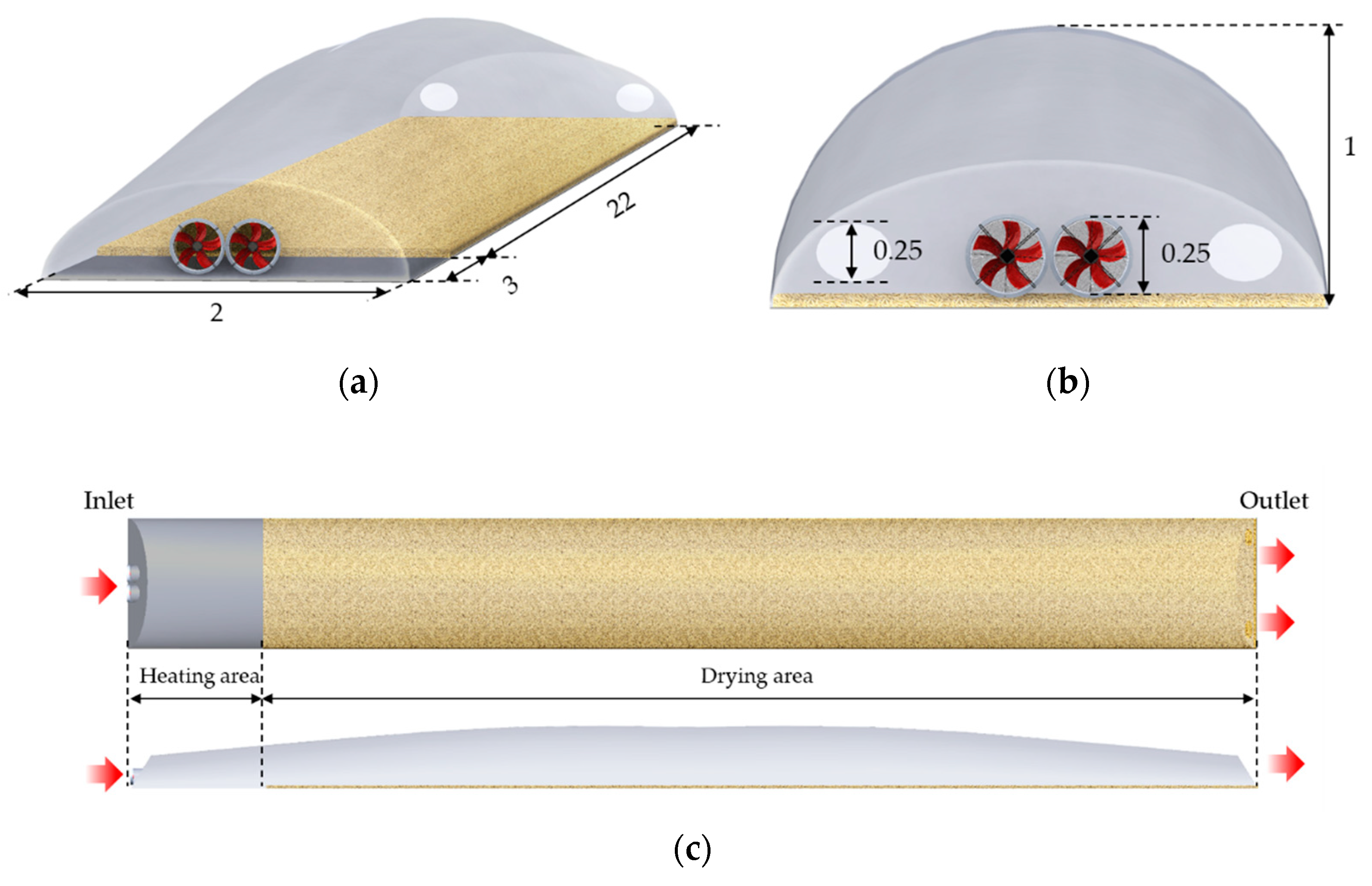
2.1. Inflatable Solar Dryer (ISD)

2.1.1. Dryer Description

The design and function of the ISD have already been described in a previous study [16]. Since then, however, the materials used to build the ISD have been reduced to a black reinforced polyvinyl chloride film (PVC, 0.52 mm) as the bottom layer, and a UV-stabilized transparent polyethylene film (PE, 150 µm) as the cover layer. A heavy-duty zipper connects the plastic films sewed along the edges of each plastic film, inflated by two axial flow ventilators of 72.6 W each, operated at 220 V (Runda Electronics CO., LTD, Shenzhen, China) (Figure 1).

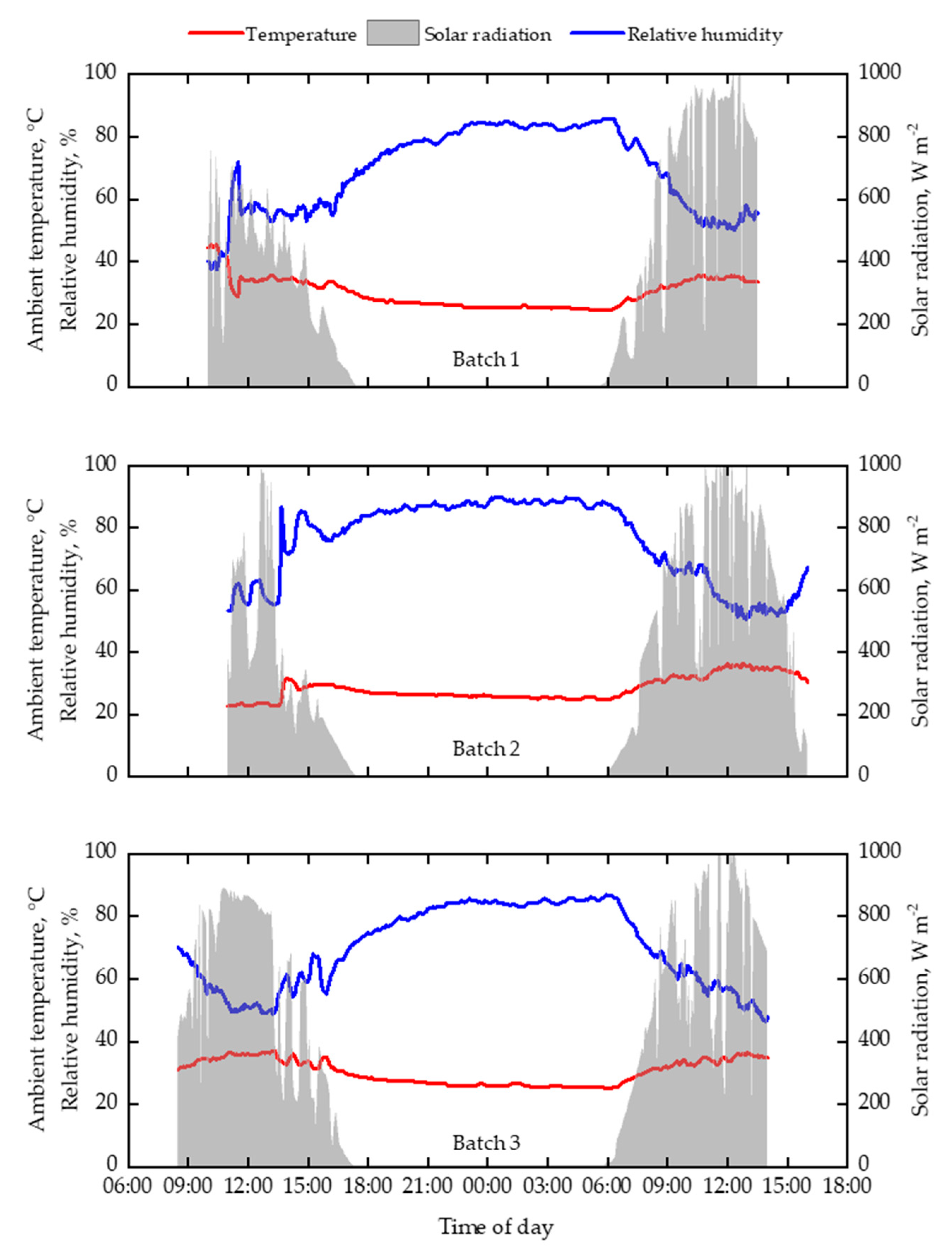
2.1.2. Field Experiments

The experiments were performed at the International Rice Research Institute (IRRI) experimental station in Los Baños, Laguna, Republic of the Philippines (14°11’N, 121°15’E, 21 m a.s.l.). Mixed rice varieties were used for the three batches of experiments during the rainy season between October and November 2013. The dryer was assembled on the ground. The two plastic films were unzipped to load the paddy rice. Then, the zipper of the dryer was closed, and the blowers were turned on to provide pressure to inflate the unit. The special roller provided for mixing the grains was pulled underneath the PVC film every hour between 8:00 and 17:00. After mixing, the moisture content was monitored. Ten grams of paddy rice was collected at three positions, as shown in Figure 2a. The samples were stored in plastic bags and transported to the IRRI laboratories. The moisture content was determined by the gravimetric method at 103 ± 2 °C for 24 h [25]. The experiments were terminated when the rice reached a target moisture content of 14% wet basis (MC_wb).

2.1.3. Instrumentation for the Field Experiments and Velocity Measurements

Solar radiation was measured using a pyranometer (CMP6, Kipp and Zonen, Delftechpark, Netherlands). Temperature and relative humidity capacity sensors (OM-EL-USB-2, Omega, Stamford, CT, USA) were placed inside the dryer at 1.5, 4, 14, 24 m from the inlet (Figure 2a). A further sensor was set to record the ambient temperature and relative humidity. The sensors were connected to a data logger (34970A, Agilent Technologies Inc., Loveland, CO, USA). The frequency of measurements was at five minutes intervals. A hot-wire anemometer (HHF42, Omega, Taipei, Taiwan) was used to measure the drying air velocity at the outlet position at one-hour intervals during the daytime.

To monitor the air velocity profile over the paddy rice, additional grid measurements were taken with the hot wire anemometer at nine positions along the dryer length and the six positions over the dryer width. The anemometer was fixed at 0.08 m above the paddy layer, facing the main airflow direction (Figure 2b). Contour plots were generated by kriging (Surfer^® 19.1.189, Golden software, Golden, CO, USA).

2.2. Simulation of Airflow Distribution in the ISD

2.2.1. Governing Equations

The differential form for a three-dimensional ISD design was simulated from the mass conservation presented according to [26]:

$$\frac{\partial {\rho }_{air}}{\partial t}+\nabla ·\left({\rho }_{air}·\overrightarrow{v}\right)=0$$

(1)

where $\overrightarrow{v}$ is the air velocity vector and ρ_air is the density of air.

The Navier–Stokes equation is represented by the momentum conservation and it is written as [26]:

$$\frac{\partial }{\partial t}\left({\rho }_{air}·\overrightarrow{v}\right)+\nabla ·\left({\rho }_{air}·\overrightarrow{v}·\overrightarrow{v}\right) =-\nabla p+\nabla ·\left(\stackrel{=}{\tau }\right)+{\rho }_{air}·g+S_m$$

(2)

where p is the static pressure, $\stackrel{=}{\tau }$ is the Reynolds stress tensor, g is the gravitational acceleration, and S_m is the source term for momentum defined as [27]:

$$S_m=\frac{150·{\left(1-ϵ\right)}^2}{d_k^2·{ϵ}^3}·{\mu }_{air}·v_{air}+\frac{1.75·{\rho }_{air}·\left(1-ϵ\right)}{d_k·{ϵ}^3}·v_{air}^2$$

(3)

where v_air is the velocity of the air, μ_air is the dynamic viscosity of air, ∈ is the porosity of paddy rice bulk and d_k is the kernel diameter. The paddy rice porosity and kernel diameter were 0.57 [28] and 1.99 mm [29]. According to ANSYS [30], the first term represents the viscous resistance, and the second term represents the inertial resistance. The corresponding values for each term were 1.634 × 10⁷ m⁻² and 2047 m⁻¹. Symbols, terms, and units for each notation in all equations are described in the nomenclature list.

2.2.2. Domain Description

The 3D geometry of the ISD used for the simulations has a total length of 25 m, where 3 m corresponds to the heating area and 22 m to the drying area (Figure 3). The inlet has a diameter of 0.25 m for each blower. Likewise, the outlets have diameters of 0.25 m. The dryer’s maximum height reached 1 m, and the paddy rice layer was set to a thickness of 0.04 m.

The fluid volume of the dryer was meshed using the ANSYS Workbench meshing tool. The mesh quality was assessed by ensuring that all elements’ skewness and element quality fell within the optimal ranges [31]. A grid independence study was performed with four mesh refinements (mesh I—813490, mesh II—1072594, mesh III—1572592, and mesh IV—2498880). Finally, mesh III was selected as a good compromise between accuracy and computation time [32].

2.2.3. CFD Model Simulation

The simulation of the airflow distribution in the ISD was carried out using ANSYS Fluent 19.1 (ANSYS Workbench, ANSYS, Inc., Canonsburg, PA, USA) installed on a HP Z420 Workstation (Hewlett-Packard, Palo Alto, CA, USA) with an Intel Xeon CPU E5-1660 3.30 GHz processor and RAM 32 GB. The simulations were performed in a steady state and the k-є realizable turbulence model was used with enhanced wall treatment. The governing equations were computed by applying a pressure-based segregated solver and the default under-relaxation factors set as solution controls. The materials used were subdivided into the fluid (drying air across the ISD) and the solid (paddy rice). The properties of incompressible gas were applied. Based on the experimental data, the calculated inlet velocity was 5 m s⁻¹. The assumptions considered in the ISD simulation were nonadiabatic and no-slip walls, as well as no shrinkage or deformation of paddy rice kernels during drying. The paddy rice bulk was considered as a porous medium.

2.3. Mathematical Modeling of the ISD

The ISD is divided into segments of one m in the direction of the airflow. The mathematical model for the ISD was developed, taking into account heat transfer in the heating area and a coupled heat and mass transfer within the drying area. The drying of paddy rice in the ISD was modeled following the approach of Hossain, et al. [22]. A schematic diagram of energy transfers inside the inflatable solar dryer is shown in Figure 4, and the following heat and mass balances are formulated.

2.3.1. Energy Balance of the Cover for the Heating Area

Figure 4 shows the energy equilibration of a control volume in the heating area. The energy balance of the cover is given as:

$$T_{cov}=\frac{{\alpha }_{cov}·\left(1+{\tau }_{cov}·{\rho }_{abs}\right)·I_t+h_w·T_{amb}}{h_w+h_{c,cov-air}+h_{r,cov-sky}+h_{r,abs-cov}}+\frac{h_{c,cov-air}·T_{air}+h_{r,cov-sky}·T_{sky}+h_{r,abs-cov}·T_{abs}}{h_w+h_{c,cov-air}+h_{r,cov-sky}+h_{r,abs-cov}}$$

(4)

where T_cov is the temperature of the cover, T_amb is the temperature of the ambient conditions, T_air is the temperature of the air, T_sky is the temperature of the sky, T_abs is the temperature of the absorber, h_w, h_c,cov-air, h_c,abs-air are the convection heat transfer coefficients between the cover and the air outside of the heating area due to wind, the cover and the air inside the heating area, and the surface of the heating area and the air inside, respectively. Additionally, h_r,abs-air and h_r,cov-air are the radiative transfer coefficients between the cover and the air outside of the heating area, and the absorber and the cover, respectively. α_cov is the absorbance of the cover, τ_cov is the transmittance of the cover, ρ_abs is the reflectance of the absorber and I_t is the instantaneous solar radiation. Complementary information on the heat transfer coefficients and how to determine them are provided in Appendix A.

2.3.2. Energy Balance of the Absorber for the Heating area

The energy balance corresponding to the heating area relates to the change over time of the energy stored in the absorber:

$$T_{abs}=\frac{\frac{{\alpha }_{abs}·{\tau }_{cov}·I_t}{1-\left(1-{\alpha }_{abs}\right)·{\rho }_{abs}}+h_{c,abs-air}·T_{air}}{h_{c,abs-air}+h_{r,sky-abs}+h_{r,abs-cov}+K_{pad-asp}}+\frac{h_{r,sky-abs}·T_{sky}+h_{r,abs-cov}·T_{cov}+K_{abs-asp}·T_{asp}}{h_{c,abs-air}+h_{r,sky-abs}+h_{r,abs-cov}+K_{abs-asp}}$$

(5)

where T_asp is the temperature of the asphalt and K_abs-asp is the thermal conductance from the absorber to the asphalt.

2.3.3. Energy Balance of the Airflow for the Heating Area

The energy balance in the air stream in the collector is given as:

$${\rho }_{air}·{\delta }_{air}·v_{air}·c_{air}·\frac{\partial T_{air}}{\partial x}=h_{c,cov-air}·\left(T_{cov}-T_{air}\right)+h_{c,abs-air}·\left(T_{abs}-T_{air}\right)$$

(6)

where δ_air is the layer thickness of the air, v_air is the air velocity, c_air is the air specific heat of air, and ∂T_air/∂x is the temperature gradient in the direction of the airflow.

The radiative and convective heat transfer coefficients were taken from Hossain, et al.’s work [22]. The convective heat transfer coefficient was computed as:

$$h_{c,cov-air}=h_{c,abs-air}=h_c=\frac{Nu·{\lambda }_{air}}{D_h}$$

(7)

where λ_air is thermal conductivity of the air, D_h is the hydraulic diameter, and Nu is the Nusselt number. The Reynolds number for a turbulent regime was calculated according to Cengel [33].

$$Nu=0.03808·R{e}^{0.8}·P{r}^{1/3}$$

(8)

where Pr is the Prandtl number and Re is the Reynolds number, which is given according to [33]:

$$Re=\frac{v_{air}·L_c}{{\mathsf{\upsilon }}_{air}}$$

(9)

where L_c is the characteristic length of the geometry and υ_air is the kinematic viscosity of air.

2.3.4. Energy Balance of the Cover in the Drying Area

According to Figure 4, the energy balance for the cover in the drying area results from the convective heat exchange between the cover and the heat transport by the drying air, which flows between the cover and the paddy rice in the drying area:

$$T_{cov}=\frac{{\alpha }_{cov}·\left(1+{\tau }_{cov}·{\rho }_{pad}\right)·I_t+h_w·T_{amb}+h_{c.cov-air}·T_{air}+h_{r,cov-sky}·T_{sky}+h_{r,pad-cov}·T_{pad}}{h_w+h_{c,cov-air}+h_{r,cov-sky}+h_{r.pad-cov}}$$

(10)

where T_pad is the temperature of paddy rice and ρ_pad is the reflectance of paddy rice.

As found in a previous study [34], the reflectance is dependent on the zenith angle (θ):

$${\rho }_{pad}=0.2704+1.816·{10}^{-5}·e^{0.1761·\theta }$$

(11)

2.3.5. Energy Balance of the Paddy Rice in the Drying Area

The change over time of the energy stored in the product results from the radiant energy on the product, the convective heat exchange between the product and the drying air, the radiant heat exchange with the cover, the environment, and the thermal losses to the ground as well as the energy required in the unit of time to evaporate the moisture. The energy balance is presented as:

$$\begin{gathered} \frac{\partial T_{pad}}{\partial t}=\frac{\frac{{\alpha }_{pad}·{\tau }_{cov}·I_t}{1-\left(1-{\alpha }_{pad}\right)·{\rho }_{pad}}+{\rho }_{pad}·{\delta }_{pad}\left(L_{pad}+\left(c_{vap}-c_{liq}\right)·T_{pad}\right)·\frac{\partial M}{\partial t}+h_{c,pad-air}·\left(T_{air}-T_{pad}\right)}{{\rho }_{pad}·{\delta }_{pad}·\left(c_{pad}+c_{liq}·M\right)} \\ +\frac{h_{r,pad-sky}·\left(T_{sky}-T_{pad}\right)+h_{r,pad-cov}·\left(T_{cov}-T_{pad}\right)+K_{pad-abs}·\left(T_{abs}-T_{pad}\right)}{{\rho }_{pad}·{\delta }_{pad}·\left(c_{pad}+c_{liq}·M\right)} \end{gathered}$$

(12)

where ρ_pad is the bulk density of paddy rice, δ_pad is the thickness of the paddy rice bulk, c_vap is the specific heat of water vapor, c_liq is the specific heat of liquid, c_pad is the specific heat of paddy rice, K_pad-abs is the thermal conductance from paddy rice to absorber, M is the moisture content dry basis (d.b.), L_pad is the latent heat of paddy rice [35] and α_pad is the absorbance of paddy rice.

2.3.6. Energy Balance of the Airflow in the Drying Area

The energy balance for the moist air in the drying area is given as:

$${\rho }_{air}·{\delta }_{air}·v_{air}·\left(c_{pad}+c_{vap}·H\right)·\frac{\partial T_{air}}{\partial x}=h_{c,cov-air}·\left(T_{cov}-T_{air}\right)+h_{c,pad-air}·\left(T_{pad}-T_{air}\right)$$

(13)

where H is the humidity ratio of air inside the dryer. The heat transfer coefficients are provided in Appendix A.

2.3.7. Energy Balance of the Bottom Layers for the Heating and Drying Area

As the ISD does not have an insulation material, the influence of the ground layers i (asphalt, soil, and absorber) is considered in the model following our previous research [34], in which the sun drying practice was modeled. The energy balance of the bottom layers under the ISD is driven by heat conduction. Figure 4 shows the thermal network across the bottom layers. The rate of thermal energy flow into the bottom layers is given as:

$$C_i·\frac{d{T}_i}{dt}=K_i·\left(T_{top}-T_i\right)+K_i·\left(T_{bottom}-T_i\right)$$

(14)

where T_i is the material temperature of the respective layer i, C_i is the thermal capacity of the material, calculated by the specific heat capacity c_i, and the thickness δ_i of the layer i:

$$C_i= c_i·{\mathsf{\delta }}_i$$

(15)

The thermal conductance K_i is given as:

$$K_i=\frac{{\lambda }_i}{\frac{1}{2}·{\mathsf{\delta }}_i}$$

(16)

where λ_i is the thermal conductivity of the material i (asphalt, soil, and absorber). The temperatures T_top and T_bottom of the layers are known boundary conditions between the layers and are given as:

$$T_{top}=\frac{K_i·T_i+K_{i+1}·T_{i+1}}{K_i+K_{i+1}}$$

(17)

$$T_{bottom}=\frac{K_i·T_i+K_{i-1}·T_{i-1}}{K_i+K_{i-1}}$$

(18)

2.3.8. Mass Balance

The moisture evaporating from the crop in the drying area is absorbed by the air. This causes a change in the enthalpy of the air, which can be described by the energy and mass balance. The rate of moisture transfer between the product and the surrounding air is expressed as:

$${\rho }_{air}·{\delta }_{air}·v_{air}·\frac{\partial H}{\partial x}·dx·dt=-{\rho }_{pad}·dx·\frac{\partial M}{\partial t}·dt$$

(19)

where ∂H/∂x is the humidity ratio and ∂M/∂t is the drying rate gradient in the direction of the airflow. The drying rate is calculated as:

$$\frac{\partial M}{\partial t}=-k·\left(M-M_e\right)$$

(20)

where M_e is the equilibrium moisture content and k is the drying constant. The calculation of M_e was obtained from the Chung–Pfost equation using the coefficients given by Iguaz and Vírseda [36]:

$$M_e=\left(-\frac{1}{0.179}\right)·ln\left(\left(-\frac{\left(\left(T_{air}-273.15\right)+16.912\right)}{277.091}\right)·ln\left(\phi \right)\right)$$

(21)

where φ is the relative humidity of the drying air.

The drying constant was obtained from paddy rice drying experiments conducted under controlled conditions. This experiment was necessary as no other paper on the subject had been reported. The drying experiments were carried out using the overflow chamber of a high-precision laboratory dryer from the Institute of Agricultural Engineering, University of Hohenheim in Stuttgart (Germany). The experimental system has been previously described in detail by Udomkun, et al. [37]. The drying experiments were conducted at air temperatures of 30, 40, 50, and 60 °C and humidity ratio of 0.020 kg kg⁻¹. The paddy rice was filled in a tray of 0.30 × 0.30 × 0.04 m having a layer thickness of 0.04 m. The paddy rice was dried to the equilibrium moisture content. The experiments were performed per triplicate for each drying condition.

The drying equation was built following three steps. The first step corresponds to the computation of the moisture ratio from the drying experiments; the second step was to obtain the drying coefficient (k) per experiment attributed to the Newton model. The third step was to fit the drying coefficient of the different experimental conditions by using an Arrhenius type equation:

$$k=4758·e^{- \frac{2987}{T_{air}}}$$

(22)

The goodness of fit for Equation (22) resulted in a coefficient of determination (R²) of 0.87 and a root mean square error (RMSE) of 0.10 h⁻¹.

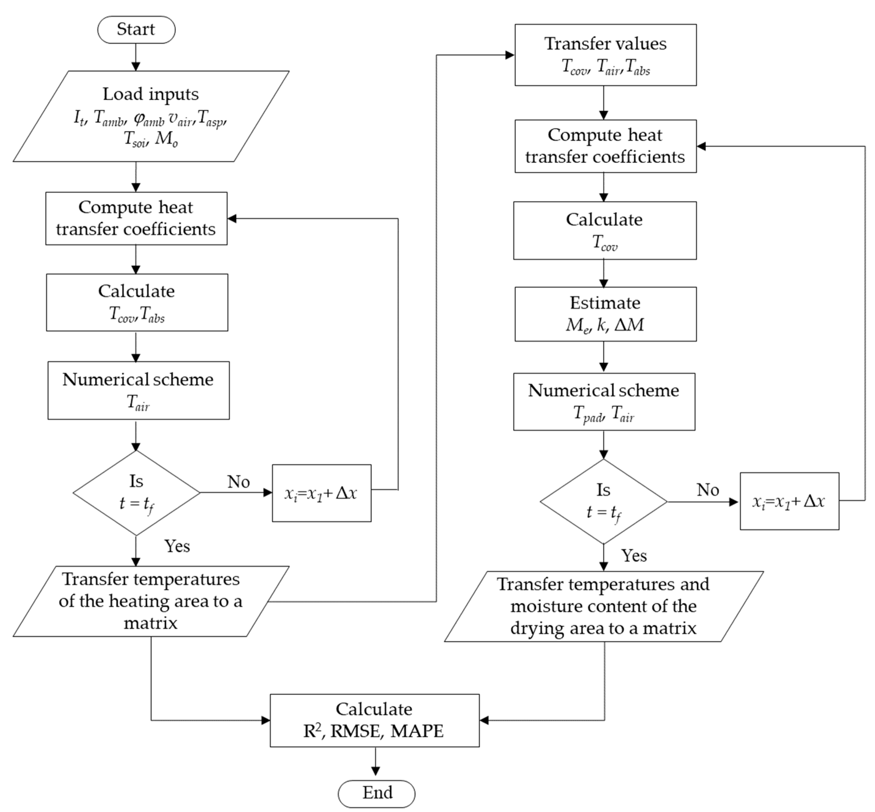
2.3.9. Solution Procedure

The partial differential equations generated for the heating area and the drying area describe heat and heat-mass transfer over small time increments. The numerical integration with respect to time and position can be solved using the finite difference method [22]. The transformation from the physical domain to the computational domain was obtained by creating a numerical simulation model of algebraic equations in one dimension. The finite volume differences of formulated heat and mass balances were replaced by the derivatives in the differential equations.

The drying air temperature given in Equation (6) was calculated over the finite distance (Δx) to give the change in air temperature in the heating area (ΔT_air) as:

$$\frac{\partial T_{air}}{\partial x}=\frac{h_{c,cov-air}·\left(T_{cov}-T_{air}\right)+h_{c,abs-air}·\left(T_{abs}-T_{air}\right)}{{\rho }_{air}·{\delta }_{air}·v_{air}·c_{air}}$$

(23)

Introducing auxiliary terms A₁ and A₂ and noting h_c for h_c,cov-air and h_c,abs-air:

$$A_1=\frac{2·h_c}{{\rho }_{air}·{\delta }_{air}·v_{air}·c_{air}} A_2=\frac{T_{cov}+T_{air}}{2}$$

(24)

leads to:

$$\Delta T_{air}=T_{air\_i}-T_{air\_i-1}=\left(A_2-T_{air\_i-1}\right)·\left(1-e^{-A_1·\mathsf{\Delta }x}\right)$$

(25)

The solution for the energy balance of the air in the drying area given in Equation (13) is solved as:

$$\frac{\partial T_{air}}{\partial x}=-A_3·T_{air}+A_4$$

(26)

where auxiliary terms A₃ and A₄ are:

$$A_3=\frac{2·h_c}{{\rho }_{air}·{\delta }_{air}·v_{air}·\left(c_{air}+c_{vap}·H\right)} A_4=\frac{T_{cov}+T_{air}}{{\rho }_{air}·{\delta }_{air}·v_{air}·\left(c_{air}+c_{vap}·H\right)}$$

(27)

leading to:

$$T_{air2}=\frac{A_4}{A_3}+\left(T_{air1}-\frac{A_4}{A_3}\right)·e^{-A_3·\mathsf{\Delta }t}$$

(28)

The temperature of paddy rice generated in Equation (12) can be solved as:

$$\frac{\partial T_{pad}}{\partial t}=-A_5·T_{pad}+A_6$$

(29)

with auxiliary terms A₅ and A₆:

$$\begin{array}{l}{A}_5=\frac{\frac{{\alpha }_{pad}·{\tau }_{cov}·I_t}{1-\left(1-{\alpha }_{pad}\right)·{\rho }_{pad}}+{\rho }_{pad}·{\delta }_{pad}·L_{pad}·\frac{\partial M}{\partial t}}{{\rho }_{pad}·{\delta }_{pad}·\left(c_{pad}+c_{liq}·M\right)}\\ +\frac{h_{c,pad-air}·T_{air}+h_{r,pad-sky}·T_{sky}+h_{r,pad-cov}·T_c+K_{pad-abs}·T_{abs}}{{\rho }_{pad}·{\delta }_{pad}·\left(c_{pad}+c_{liq}·M\right)}\\ A_6=-\frac{-{\rho }_{pad}·{\delta }_{pad}·\left(c_{vap}-c_{liq}\right)·\frac{\partial M}{\partial t}+h_{c,pad-air}+h_{r,pad-sky}+h_{r,pad-cov}+K_{pad-abs}}{{\rho }_{pad}·{\delta }_{pad}·\left(c_{pad}+c_{liq}·M\right)}\end{array}$$

(30)

leading to:

$$T_{pad2}=\frac{A_6}{A_5}+\left(T_{pad1}-\frac{A_6}{A_5}\right)·e^{-A_5·\mathsf{\Delta }t}$$

(31)

The rate of change of moisture content inside the dryer is represented in the finite difference form according to Bala [35]:

$$\mathsf{\Delta }M=\frac{-k·\left(M-M_e\right)·\mathsf{\Delta }t}{1+\frac{k}{2}·\mathsf{\Delta }t}$$

(32)

The change of humidity solution can be calculated as:

$$\mathsf{\Delta }H=-\left(\frac{{\rho }_{pad}}{b·{\rho }_{air}·{\delta }_{air}·v_{air}}\right)· \left(\frac{\mathsf{\Delta }M}{\mathsf{\Delta }t}\right)·\mathsf{\Delta }x$$

(33)

Table 1. Properties of the materials.

Description	Value	Unit
Cover [38]
Density ρcov	920.0	kg m−3
Specific heat ccov	2200.0	J kg−1 K−1
Thermal conductivity λcov	0.24	W m−1 K−1
Absorber [38]
Density ρabs	1300.0	kg m−3
Specific heat cabs	1500.0	J kg−1 K−1
Thermal conductivity λabs	0.14	W m−1 K−1
Paddy rice [28]
Density ρpad	609.0	kg m−3
Specific heat cpad	2000.0	J kg−1 K−1
Thermal conductivity λpad	0.12	W m−1 K−1
Asphalt [39]
Density ρasp	2282.0	kg m−3
Specific heat casp	959.0	J kg−1 K−1
Thermal conductivity λasp	1.30	W m−1 K−1
Soil [40]
Density ρsoi	2650.0	kg m−3
Specific heat csoi	870.0	J kg−1 K−1
Thermal conductivity λsoi	2.50	W m−1 K−1

presents the material properties of the ISD, the paddy rice, and the ground layers used for the MATLAB/Simulink^® model.

MATLAB/Simulink^® 2019a (MathWorks Inc., Natick, MA, USA) was used to compute the temperatures and the moisture content behavior of the paddy rice drying inside the ISD. The lumped equations are a set of partial differential equations that are converted to coupled ordinary equations to solve using Simulink graphical interface [41]. The flowchart of the solution is illustrated in Figure 5. The coefficient of determination (R²), the root mean square error (RMSE), and mean absolute percentage error (MAPE) were used to assess the accuracy of prediction models.

2.4. Model Implementation

The weather data were collected from the weather station at the experimental station of the International Rice Research Institute in Los Baños, Laguna, Republic of the Philippines at 14°11′ N, 121°15′ E. The annual weather records from 2008 to 2017 were collected from the weather station every 15 min. Ambient temperature, relative humidity, and daily solar radiation data were averaged (see Figure 6). The weather data were used for the model implementation corresponding to the peak harvest season for the dry season (April and May) and the rainy season (October and November).

Table 2. Initial values for the ISD model.

Parameter	Dry Season	Rainy Season
Moisture content w.b., %	18.0	22.5
Humidity ratio, kg kg−1	0.015	0.020
Drying time, h	32	48

shows the initial values for the ISD model in MATLAB/Simulink.

3. Results

3.1. CFD Simulations

3.1.1. Simulation of the Airflow Distribution

The simulation of the airflow pattern in the inflatable solar dryer (ISD) is shown in Figure 7, where the airflow direction travels from left to right. Figure 7a shows the vortex caused by the fans located at the inlet. The vortex covers the first meters of the ISD, where the air velocity is the highest (Figure 7b). Furthermore, the airflow in the drying area forms a transition zone, where the airflow presents an even distribution over the paddy rice. However, backflow was observed one meter before exiting the dryer. The turbulence model k-є predicted the presence of the air turbulence in the area located at 3 to 4 m from the fans well, creating a recirculation pattern.

3.1.2. Validation of the CFD Model

A contour plot was used to compare the CFD simulation and the experimental values and to analyze the airflow distribution over the paddy rice (Figure 8). The simulated results were consistent with Figure 7. Thus, the airflow velocity was higher at the left side. It can be seen that the air velocity profile at 0.08 m decreased in the heating area from 5.0 to 0.5 m s⁻¹, and the velocity in the drying area was around 0.1 m s⁻¹.

Figure 9 shows the computational and experimental velocities over the ISD’s length. The results indicate that air velocity decreased along the dryer length and that air velocity magnitude in the x-direction at 0.08 m above the paddy rice verifies the computational results with the experimental data. The comparison with the computed and experimental data revealed a good correlation, with a R² of 0.78 and a RMSE of 0.72 m s⁻¹.

3.2. Validation of the Drying Model

3.2.1. Simulation of the Air Temperature during the Drying Process

Figure 10 presents the solar radiation, the ambient temperature, and the relative humidity during the three experimental batches of solar drying of paddy rice in the ISD. The solar radiation during the rainy season shows higher variations due to clouds and sudden rainfall. When the sun rises, the ambient relative humidity declines gradually and keeps to a minimum value of 55% at around noon. This corresponds to the maximum temperature of 36 °C. The ambient temperature during nighttime reaches about 22 °C, while the relative humidity increases to 88%.

The simulated temperature was validated against the experimental paddy rice data, as shown in Figure 11. It can be observed that the temperature increase in the drying area was well reproduced throughout the drying process. During the daytime, the average drying air temperatures varied from 5 to 25 °C above the ambient temperature. The highest experimental and simulated drying temperatures were 63.7 and 60.2 °C at 13:05 and 12:00, respectively. The high fluctuation of weather conditions such as cloudiness or sudden showers influenced the temperature in the ISD. This phenomenon can be also observed from the simulated temperature. Therefore, the simulation was in good agreement with experimental data.

3.2.2. Simulation of the Moisture Content during the Drying Process

Figure 12 shows the comparison between the experimental and predicted moisture contents during solar drying of paddy rice in the ISD. Rewetting during night or rainy hours was not observed as the fans were operating continuously. The target moisture content was reached with the ISD between 27 and 29.5 h according to the experimental values. From the experimental data, it can be seen that increased fluctuation of weather conditions strongly influences the drying behavior of paddy rice. Nevertheless, the simulation model could effectively predict the moisture content changes during drying, particularly under good weather conditions, as shown in batch 3.

3.2.3. Accuracy of the Model

The goodness of fit of the simulation model is presented in

Table 3. Model constants and statistic criteria (moisture content wet basis—MC_wb, coefficient of determination—R², root mean square error root mean square error—RMSE and the mean absolute percentage error—MAPE).

Batch	Date	Drying Period h	Initial MCw.b. %	Variables	R2	RMSE °C, %	MAPE %
1	30 October 2013	27.0	22.3	Tabs	0.85	2.7	1.5
				Tpad	0.73	5.8	6.5
				MCw.b	0.82	1.4	7.4
2	5 November 2013	29.0	22.5	Tabs	0.91	2.7	0.2
				Tpad	0.79	6.6	6.3
				MCw.b	0.84	1.2	3.1
3	15 November 2013	29.5	22.5	Tabs	0.90	2.2	0.4
				Tpad	0.85	5.1	6.9
				MCw.b	0.96	0.5	0.9

. High accuracy can be observed from the temperature in the heating area and the outlet, as well as the moisture content of the paddy rice during drying. The highest R² can be observed from batch 3 where the weather conditions were stable, especially the first day compared to the other batches. For the three batches, the RMSE for temperature was less than 6.6 °C and 1.4% for moisture content. In general, the MAPE for temperatures is below 6.9%, while the MAPE of moisture content is below 7.4%. As the MAPE of the simulation model was still below 10%, high prediction accuracy was therefore proven [42].

3.2.4. Application of the Model

Figure 13a shows the simulated moisture content during the relevant months in the dry season and the rainy season for the 10-year period (2008–2017). Figure 13b summarizes the average drying time for the dry season and the rainy season, where 14% MC_wb was achieved. The prediction shows that during the dry season, the target moisture content can be reached within 10 h, while during the rainy season, the drying time increases, and the drying time may be higher than 30 h.

4. Discussion

The current study investigated the airflow patterns in the ISD. The results obtained with the CFD simulation model helped to visualize the airflow distribution (Figure 7). A velocity reduction is expected due to an abrupt expansion from the fan to the dryer. These results are likely to be related to a turbulent regime [43] and generated vortex in the heating area, as seen in Figure 7a. A similar flow structure has been shown in another study [44].

Previous studies evaluating the airflow patterns in solar dryers have been conducted using a CFD approach [21,45,46], where the study of the turbulence effect was proportionally related to the rate of heat transfer. This effect was also observed in the ISD where the presence of higher velocity in the heating area and lower velocities over the paddy rice spread along the drying area shows a temperature rise across the dryer (Figure 11b).

The simulated results from the MATLAB/Simulink model are consistent with the experimental data (Figure 11). A similar behavior was also observed from drying various agricultural products using the Hohenheim solar tunnel dryer type [23,47,48,49,50].

Several studies have reported different simulation models of forced convection solar drying systems, where a thin layer of drying materials was commonly assumed and described [22,23,51]. In this study, we have used the same approach and have further developed the drying kinetics of paddy rice. For example, we show that the prediction of moisture content during drying is more accurate compared to the prediction of temperatures (Table 3). Based on the results, the drying process in the ISD can be computationally evaluated with a good agreement to the empirical measurements.

The results of the application of the model over the dry and the rainy seasons further support the results of the previous ISD experiments [16], where drying during the rainy season required a long period of time, while in the dry season it was accomplished within 10 h of the drying process. Further research should be undertaken with ANSYS fluent and MATLAB/Simulink to investigate the application of the collaborative model approach with different agricultural commodities and weather conditions.

5. Conclusions

This study presents CFD-Simulink models used to simulate and predict the ISD’s performance when drying paddy rice. The airflow patterns were successfully investigated across the ISD using a CFD approach via ANSYS Fluent. A good agreement was revealed between the CFD simulation and experimental velocity measurements with an R² of 0.78 and RMSE of 0.72 m s⁻¹. A variation of air velocity from 5 to 0.5 m s⁻¹ and 0.5 to 0.1 m s⁻¹ was obtained at the heating and drying area, respectively. A vortex was observed from 3 to 4 m in the heating area caused by the air conveyance of the axial fans. Moreover, we successfully modeled the drying process of paddy rice using the MATLAB/Simulink. A good agreement between the experimental and the simulated moisture contents of paddy rice (R² > 0.82, RMSE < 1.4 °C, MAPE < 7.4%) and temperatures (R² > 0.73, RMSE < 6.6%, MAPE < 6.9%) was achieved. The validated model allowed an accurate assessment of the drying behavior of paddy rice over the rainy and dry seasons to be made.

The CFD-Simulink models proved to be an efficient and effective means of simulating and assessing the ISD’s performance under different weather conditions. The computational approach used in this study shows great potential as a decision support tool to improve the ISD design. Further investigations should include the mixing effect of paddy rice during drying and the ratio of heating and drying area.

References

1. Papademetriou, M.K.; Dent, F.J.; Herath, E.M. Bridging the Rice Yield Gap in the Asia-Pacific Region; FAO Regional Office for Asia and the Pacific: Bangkok, Thailand, 2000.
2. GRISP (Global Rice Science Partnership). Rice Almanac. In Source Book for One of the Most Important Economic Activities on Earth, 4th ed.; International Rice Research Institute: Los Baños, Philippines, 2013. [Google Scholar]
3. Manandhar, A.; Milindi, P.; Shah, A. An overview of the post-harvest grain storage practices of smallholder farmers in developing countries. Agriculture 2018, 8, 57. [Google Scholar] [CrossRef] [Green Version]
4. Chen, G. Advances in Agricultural Machinery and Technologies, 1st ed.; CRC Press: Boca Raton, FL, USA, 2018. [Google Scholar]
5. Mopera, L.E. Food Loss in the Food Value Chain: The Philippine Agriculture Scenario. J. Dev. Sustain. Agric. 2016, 11, 8–16. [Google Scholar] [CrossRef]
6. Abdullah, S.N.A.; Chai-Ling, H.; Wagstaff, C. Crop Improvement: Sustainability through Leading-Edge Technology; Springer International Publishing AG: Cham, Switzerland, 2017. [Google Scholar]
7. Tsotsas, E.; Mujumdar, A.S. Modern Drying Technology, Volume 3: Product Quality and Formulation; Wiley: Hoboken, NJ, USA, 2011. [Google Scholar]
8. Ulep, M.C.; Casil, F.B.; Castro, R.C.; Gagelonia, E.C.; Bautista, E.U. Technical and socio-economic evaluation in Ilocos Norte of a low-cost grain dryer from Vietnam. Philipp. J. Crop Sci. 2004, 29, 5–15. [Google Scholar]
9. Djokoto, I.K.; Maurer, R.; Muehlbauer, W. Solar tunnel dryer for drying paddy. AMA 1989, 20, 41–43. [Google Scholar]
10. Chupungco, A.; Dumayas, E.; Mullen, J. Two-Stage Grain Drying in the Philippines; ACIAR: Canberra, Australia, 2008; p. 50.
11. Romulado, M. Modelling and Simulation of the Two-Stage Rice Drying System in the Philippines. Ph.D. Thesis, Agricultural Engineering University of Hohenheim, Stuttgart, Germany, 2001. [Google Scholar]
12. Gummert, M. Improved postharvest technologies and management for reducing postharvest losses in rice. Acta Horticult. 2013, 1011, 63–70. [Google Scholar] [CrossRef]
13. Rodriguez, A.; Paz, R. Factors affecting the use of mechanical dryers. In Partnerships for Modernizing the Grain Postproduction Sector; Bakker, R., Borlagdan, P., Hardy, B., Eds.; International Rice Research Institute: Los Baños, Philippines, 2004; pp. 51–56. [Google Scholar]
14. Cardino, A. Case studies of mechanical dryers in the Philippines: Lessons learned. In Small Farm Equipment for Developing Countries; International Rice Research Institute: Los Baños, Philippines, 1986; pp. 431–437. [Google Scholar]
15. Maurer, R. Untersuchung Und Modifikation Einer Solaren Tunneltrocknungsanlage Mit Integriertem Kollektor Für Den Einsatz Bei Der Reistrocknung in Humiden Gebieten. Diplom Thesis, Agricultural Engineering University of Hohenheim, Stuttgart, Germany, 1989. [Google Scholar]
16. Salvatierra-Rojas, A.; Nagle, M.; Gummert, M.; de Bruin, T.; Müller, J. Development of an inflatable solar dryer for improved postharvest handling of paddy rice in humid climates. Int. J. Agric. Biol. Eng. 2017, 10, 269–282. [Google Scholar] [CrossRef]
17. Romuli, S.; Schock, S.; Somda, M.K.; Müller, J. Drying performance and aflatoxin content of paddy rice applying an inflatable solar dryer in Burkina Faso. Appl. Sci. 2020, 10, 3533. [Google Scholar] [CrossRef]
18. Romuli, S.; Schock, S.; Nagle, M.; Chege, C.G.K.; Müller, J. Technical performance of an inflatable solar dryer for drying amaranth leaves in Kenya. Appl. Sci. 2019, 9, 3431. [Google Scholar] [CrossRef] [Green Version]
19. van Hung, N.; Fuertes, L.A.; Balingbing, C.; Roxas, A.P.; Tala, M.; Gummert, M. Development and performance investigation of an inflatable solar drying technology for oyster mushroom. Energies 2020, 13, 4122. [Google Scholar] [CrossRef]
20. Asemu, A.M.; Habtu, N.G.; Delele, M.A.; Subramanyam, B.; Alavi, S. Drying characteristics of maize grain in solar bubble dryer. J. Food Process Eng. 2020, 43, 3312. [Google Scholar] [CrossRef]
21. Ghaffari, A.; Mehdipour, R. Modeling and Improving the Performance of Cabinet Solar Dryer Using Computational Fluid Dynamics. Int. J. Food Eng. 2015, 11, 157–172. [Google Scholar] [CrossRef]
22. Hossain, M.A.; Woods, J.L.; Bala, B.K. Simulation of solar drying of chilli in solar tunnel drier. Int. J. Sustain. Energy 2005, 24, 143–153. [Google Scholar] [CrossRef]
23. Janjai, S.; Lamlert, N.; Intawee, P.; Mahayothee, B.; Boonrod, Y.; Haewsungcharern, M.; Bala, B.K.; Nagle, M.; Müller, J. Solar drying of peeled longan using a side loading type solar tunnel dryer: Experimental and simulated performance. Dry. Technol. 2009, 27, 595–605. [Google Scholar] [CrossRef]
24. Esper, A. Solarer tunneltrockner mit photovoltaischem antriebssystem. Ph.D. Thesis, Agricultural Engineering University of Hohenheim, Stuttgart, Germany, 1995. [Google Scholar]
25. Chen, C. Evaluation of Air Oven Moisture Content Determination Methods for Rough Rice. Biosyst. Eng. 2003, 86, 447–457. [Google Scholar] [CrossRef]
26. ANSYS. ANSYS FLUENT Theory Guide; ANSYS Inc.: Canonsburg, PA, USA, 2011. [Google Scholar]
27. Sanghi, A.; Ambrose, R.P.K.; Maier, D. CFD simulation of corn drying in a natural convection solar dryer. Dry. Technol. 2018, 36, 859–870. [Google Scholar] [CrossRef]
28. Iguaz, A.; San Martín, M.B.; Arroqui, C.; Fernández, T.; Maté, J.I.; Vírseda, P. Thermophysical properties of medium grain rough rice (LIDO cultivar) at medium and low temperatures. Eur. Food Res. Technol. 2003, 217, 224–229. [Google Scholar] [CrossRef]
29. Lee, C.; Chung, D. Grain physical and thermal properties related to drying and aeration. In Grain Drying in Asia; Champ, B.R., Highley, E., Johnson, G.I., Eds.; Australian Centre for International Agricultural Research: Bangkok, Thailand, 1996; p. 410. [Google Scholar]
30. ANSYS. Cell Zone and Boundary Conditions. In ANSYS Fluent User’s Guide. Release 15.0; ANSYS, Inc.: Canonsburg, PA, USA, 2013. [Google Scholar]
31. ANSYS. User Guide. Available online: https://www.afs.enea.it/project/neptunius/docs/fluent/html/ug/node167.htm (accessed on 15 September 2020).
32. Drück, H.; Mathur, J.; Panthalookaran, V.; Sreekumar, V.M. Green Buildings and Sustainable Engineering: Proceedings of GBSE 2019; Springer: Singapore, 2020. [Google Scholar]
33. Çengel, Y.A. Heat Transfer: A Practical Approach; McGraw-Hill: New York, NY, USA, 2003. [Google Scholar]
34. Salvatierra-Rojas, A.; Torres-Toledo, V.; Müller, J. Influence of surface reflection (Albedo) in simulating the sun drying of paddy rice. Appl. Sci. 2020, 10, 5092. [Google Scholar] [CrossRef]
35. Bala, B.K. Solar Drying Systems: Simulations and Optimization; Agrotech Publishing Academy: Mymensingh, Bangladesh, 1998. [Google Scholar]
36. Iguaz, A.; Vírseda, P. Moisture desorption isotherms of rough rice at high temperatures. J. Food Eng. 2007, 79, 794–802. [Google Scholar] [CrossRef]
37. Udomkun, P.; Argyropoulos, D.; Nagle, M.; Mahayothee, B.; Janjai, S.; Müller, J. Single layer drying kinetics of papaya amidst vertical and horizontal airflow. LWT 2015, 64, 67–73. [Google Scholar] [CrossRef]
38. Crawford, R.J. Plastics Engineering; Elsevier Science: Amsterdam, The Netherlands, 2013. [Google Scholar]
39. Bai, B.C.; Park, D.W.; Vo, H.V.; Dessouky, S.; Im, J.S. Thermal Properties of Asphalt Mixtures Modified with Conductive Fillers. J. Nanomater. 2015, 2015, 926809. [Google Scholar] [CrossRef] [Green Version]
40. Campbell, G.S.; Norman, J. An Introduction to Environmental Biophysics; Springer: New York, NY, USA, 2012. [Google Scholar]
41. Gran, R.J. Numerical Computing with Simulink, Volume 1: Creating Simulations; Society for Industrial and Applied Mathematics: Philadelphia, PA, USA, 2007. [Google Scholar]
42. Yadav, A.K.; Chandel, S.S. Solar radiation prediction using Artificial Neural Network techniques: A review. Renew. Sustain. Energy Rev. 2014, 33, 772–781. [Google Scholar] [CrossRef]
43. Burgess, W.A.; Ellenbecker, M.J.; Treitman, R.D. Ventilation for Control of the Work Environment; Wiley: Hoboken, NJ, USA, 2004. [Google Scholar]
44. Bournet, P.E.; Boulard, T. Effect of ventilator configuration on the distributed climate of greenhouses: A review of experimental and CFD studies. Comput. Electron. Agric. 2010, 74, 195–217. [Google Scholar] [CrossRef]
45. Lokeswaran, S.; Eswaramoorthy, M. An experimental analysis of a solar greenhouse drier: Computational Fluid Dynamics (CFD) validation. Energy Sources Part A Recovery Util. Environ. Effects 2013, 35, 2062–2071. [Google Scholar] [CrossRef]
46. Milczarek, R.R.; Alleyne, F.S. Mathematical and computational modeling simulation of solar drying systems. In Solar Drying Technology; Springer Singapore: Singapore, 2017; pp. 357–379. [Google Scholar] [CrossRef]
47. Bala, B.K.; Mondol, M.R.A. Experimental investigation on solar drying of fish using solar tunnel dryer. Dry. Technol. 2001, 19, 427–436. [Google Scholar] [CrossRef]
48. Bala, B.K.; Mondol, M.R.A.; Biswas, B.K.; Das Chowdury, B.L.; Janjai, S. Solar drying of pineapple using solar tunnel drier. Renew. Energy 2003, 28, 183–190. [Google Scholar] [CrossRef]
49. Schirmer, P.; Janjai, S.; Esper, A.; Smitabhindu, R.; Mühlbauer, W. Experimental investigation of the performance of the solar tunnel dryer for drying bananas. Renew. Energy 1996, 7, 119–129. [Google Scholar] [CrossRef]
50. Lutz, K.; Mühlbauer, W.; Müller, J.; Reisinger, G. Development of a multi-purpose solar crop dryer for arid zones. Solar Wind Technol. 1987, 4, 417–424. [Google Scholar] [CrossRef]
51. Bala, B.K.; Woods, J.L. Simulation of the indirect natural convection solar drying of rough rice. Sol. Energy 1994, 53, 259–266. [Google Scholar] [CrossRef]
52. ASHRAE. Fundamentals Handbook; ASHRAE: Atlanta, GA, USA, 2001. [Google Scholar]
53. Thorpe, G.R. The application of computational fluid dynamics codes to simulate heat and moisture transfer in stored grains. J. Stored Prod. Res. 2008, 44, 21–31. [Google Scholar] [CrossRef]
Figure 1. Inflatable solar dryer: (a) perspective view and (b) inside of the dryer.
Applsci 11 03118 g001
Figure 2. Position of measuring devices for (a) solar drying experiments (solar radiation, temperature, relative humidity, moisture content, and velocity) and (b) velocity measuring points across the dryer.
Applsci 11 03118 g002
Figure 3. Inflatable solar dryer (ISD) computational geometry: (a) isometric, (b) front, (c) top and side view (dimensions are shown in m).
Applsci 11 03118 g003
Figure 4. Schematic diagram of heat balances in the (a) heating area and (b) drying area of the ISD ( Applsci 11 03118 i001—radiation, Applsci 11 03118 i002—convection, and ⟶—conduction).
Applsci 11 03118 g004
Figure 5. Simulation procedure flowchart.
Applsci 11 03118 g005
Figure 6. Annual weather data from the weather station at the International Rice Research Institute (IRRI) (averaged values 2008−2017).
Applsci 11 03118 g006
Figure 7. 3D streamlines of airflow in the ISD: (a) top view and (b) side view with zoomed view of the heating area.
Applsci 11 03118 g007
Figure 8. Contour plots of the simulated and experimental airflow distribution at the height of 0.08 m across the ISD.
Applsci 11 03118 g008
Figure 9. Simulated and experimental air velocity along the centerline at the height of 0.08 m over the ISD length.
Applsci 11 03118 g009
Figure 10. The variation of ambient temperature, relative humidity, and solar radiation for the three experimental batches during rainy season.
Applsci 11 03118 g010
Figure 11. Simulated (a) and experimental (b) temperature profile over time and along the length of the ISD of the 3 experimental batches.
Applsci 11 03118 g011
Figure 12. Experimental and simulated moisture content in the ISD during paddy rice drying of three experimental batches (red line indicates target MCwb = 14%).
Applsci 11 03118 g012
Figure 13. Simulated outputs of the ISD drying model using the weather data from the experimental station of the International Rice Research Institute in Los Baños, Laguna, Republic of the Philippines (average 2008–2017); (a) drying curves corresponding to the peak harvesting months of the dry season and the rainy seasons and (b) drying time obtained for a target MCwb = 14% from each harvest season.
Applsci 11 03118 g013