Article

End-to-End Deep Reinforcement Learning for Decentralized Task Allocation and Navigation for a Multi-Robot System  †

by
Ahmed Elfakharany
*,‡ and
Zool Hilmi Ismail
*,‡
Center for Artificial Intelligence & Robotics, Malaysia Japan International Institute of Technology, Universiti Teknologi Malaysia, Jalan Sultan Yahya Petra, Kuala Lumpur 54100, Malaysia
*
Authors to whom correspondence should be addressed.
This paper is an extended version of our paper published in The Fourth International Conference on Advanced Technology and Applied Sciences (ICaTAS 2019), Cairo, Egypt, 10–12 September 2019.
These authors contributed equally to this work.
Appl. Sci. 2021, 11(7), 2895; https://doi.org/10.3390/app11072895
Submission received: 31 December 2020 / Revised: 13 March 2021 / Accepted: 15 March 2021 / Published: 24 March 2021
(This article belongs to the Special Issue Applications of Intelligent Control Methods in Mechatronic Systems)

Abstract

:
In this paper, we present a novel deep reinforcement learning (DRL) based method that is used to perform multi-robot task allocation (MRTA) and navigation in an end-to-end fashion. The policy operates in a decentralized manner mapping raw sensor measurements to the robot’s steering commands without the need to construct a map of the environment. We also present a new metric called the Task Allocation Index ( T A I ), which measures the performance of a method that performs MRTA and navigation from end-to-end in performing MRTA. The policy was trained on a simulated gazebo environment. The centralized learning and decentralized execution paradigm was used for training the policy. The policy was evaluated quantitatively and visually. The simulation results showed the effectiveness of the proposed method deployed on multiple Turtlebot3 robots.

1. Introduction

Classical multi-robot systems (MRS) usually have two main steps: task allocation and task execution. In the context of multiple homogeneous mobile robots in which the tasks being executed are reaching multiple goal positions, the two main MRS steps become multi-robot task allocation (MRTA) and navigation. The MRTA algorithm’s role is to assign tasks to robots in order to decrease the total cost exerted by all of the robots [1]. On the other hand, the navigation part usually includes multi-robot path planning algorithms (MPPs) [2], which plan paths for multiple robots to avoid any collisions between the robots or other obstacles. The problem arising due to the decoupling of both algorithms is that most MRTA algorithms do not adjust for any cost changes in the paths of the robots [3] due to multiple reasons, for example: dynamic obstacles or partial observability.
Reinforcement learning (RL) is a branch of machine learning in which an agent is interacting with the environment by receiving a state from the environment, then taking an action. There is a reward signal that signals the quality of the action. The goal of an RL algorithm is to learn through a heuristic approach how to maximize not only the immediate reward, but also the subsequent rewards [4]. One of the drawbacks of RL algorithms is their lack of scalability in terms of the dimensionality of the state of the environment; thus, their use is limited to solving low-dimensional problems [5]. The rise of deep neural networks as a powerful tool that can learn to find compact features of high-dimensional data has led to the introduction of the field of deep reinforcement learning (DRL) [5].
Researchers in the field of multi-robot systems (MRS) became attracted to DRL due to its ability to handle high-dimensional data [6] and the fact that RL algorithms are model free and have the ability to handle nonlinear, stochastic dynamics and non-quadratic reward functions [7]. As for the MRTA problem, researchers have used DRL to solve the MRTA problem, especially the fairness of the allocation problem [8] and the dynamic task allocation problem [9]. On the other hand, the use of DRL to solve the navigation problem has been given more attention by researchers due to DRL’s ability to learn decentralized policies that can drive an MRS towards its goal positions [10,11,12,13]. As far as we know, there is a gap in the literature where there have not been any proposed methods that combine both MRTA and navigation.
In this paper, we propose a novel method that combines both MRTA and navigation for a homogeneous multi-robot system. The method is a decentralized deep reinforcement learning policy whose inputs are the raw sensor measurements and whose outputs are the robot’s steering commands. The output of the policy should drive the robot from its initial position to a unique goal position without colliding with other robots or obstacles. We demonstrate that our method learned to perform both MRTA and navigation from end-to-end effectively, and we compare our method to two methods from the literature that only perform decentralized navigation for a multi-robot system. Thus, this paper is a first step to address performing MRTA and navigation from end-to-end and shows promising results that can be built on to enhance the current state of multi-robot systems.
The main contributions of this paper are:
  • An introduction of a novel method that performs MRTA and navigation for a homogeneous multi-robot system from end-to-end using deep reinforcement learning.
  • An introduction of a new metric called the Task Allocation Index ( T A I ), which measures the performance of navigation in MRTA.

2. Related Works

Recently, Zhu et al. [8] attempted to solve the fairness of allocation problem for a team of heterogeneous robots with different capabilities to perform the tasks. The problem they attempted to solve is an ST-MR-IAMRTA problem. They modeled the capability of a robot as a resource used to accomplish the task. When for a group of tasks, each of them requests a group of resources, the problem of the fairness of allocation arises. In order to solve the fairness problem, each resource requester (task) should be allocated the resources optimally to maximize the satisfaction of resource requesters. Zhu et al. [8] developed a decentralized two-phase algorithm. The first phase is the resource requester selection, which was modeled as a coordination game and solved using a deep Q-network (DQN) [14], which was used to learn the optimal strategies. The second phase is a consensus based algorithm for forming a team of robots to solve the task, thus only solving the MRTA problem without addressing the navigation problem.
Chen et al. [10] used a DRL algorithm that performs decentralized multi-agent collision avoidance. The DRL algorithm they used is a value network that uses the agent’s joint configuration (positions and velocities) and the joint configurations of the other agents to encode the estimated time to the given goal position. The advantage of using the value network is its ability to run in real time and consider the uncertainty in the other agent’s motion to predict a collision-free velocity vector. Chen et al. [10] designed their algorithm to work in cases of unreliable communication between the agents, which requires the value network to inherently predict the other agents’ intents. Hence, the other agents’ states are calculated using the agent’s sensor measurements. They modeled static obstacles as stationary agents. They formulated the problem as a partially observable sequential decision making problem. The value network was first trained by using supervised learning (back-propagation) on a training dataset consisting of 500 trajectories generated using the optimal reciprocal collision avoidance (ORCA) algorithm [15], then the trained weights were used as the initialization to the DRL training. The value network was trained using a modified Q-learning update [4]. A major drawback of the paper is that by treating obstacles as stationary agents, the input size to the neural network increases with the increase of the number of obstacles, leading to the network being impractical in environments with a large number of obstacles. It is obvious from the paper that the value network effectively performs navigation with both decentralized MPP and path tracking, but does not address the MRTA problem.
On the other hand, Lin et al. [11] developed a novel DRL method to navigate a team of robots through an unknown environment. The aim of the method is drive a robot team such that their geometric centroid reaches a goal position while avoiding collisions and maintaining connectivity between the robots. The robots need to be within a certain distance from each other to maintain the connectivity between them. The centralized learning and decentralized execution were the mechanisms used to train the policy neural network in which each robot has a copy of the policy network controlling it. The policy network takes the raw readings of a 2D laser scanner, the goals’ relative position, and other robots’ relative positions as the inputs and outputs continuous velocity controls. They designed the reward function to be reaching the goal position, maintaining connectivity, and achieving smooth motion, while it penalizes collisions. They trained their policy network using proximal policy optimization (PPO) [16]. The paper only addressed the issue of making the geometric centroid of the robot team reach the goal position and did not address each robot’s terminal goal position.
Long et al. [12] developed a decentralized sensor level collision avoidance algorithm for an MRS. The policy is a deep neural network (DNN) that maps directly between raw sensor measurements to a differential robot’s linear and rotational velocities in order to drive the robot towards its goal position. The policy network is decentralized in a way that each robot has a copy of the network. At each time step, the policy network receives an observation that consists of the readings of a 2D laser scanner, the goal’s position relative to the robot, and the robot’s current linear and rotational velocities. The action space from which the policy network samples the output is a continuous space in which the linear velocity is in the range between [0.0, 1.0] and the rotational velocity is in the range between [−1.0, 1.0]. Hence, the problem is formulated as a partially observable Markov decision process (POMDP) [17]. They trained their neural network using proximal policy optimization (PPO) [16]. They adapted the centralized learning, decentralized execution paradigm in which each robot collects its own experiences (observations, actions, rewards) and the policy is trained on the collective experiences gathered by all the robots. It is obvious from the paper that it is similar to the approach used by Chen et al. [10] in which the policy network effectively preforms navigation with both decentralized MPP and path tracking when the goal positions are set for each robot, but the paper did not address the MRTA problem.
Fan et al. [13] published subsequent work to Long et al.’s [12] work, in which they validated Long et al.’s policy in real-world setups. They made two observations. The first is that Long et al.’s policy does not perform optimally in some trivial situations in which there are no obstacles or other agents nearby or when a robot is near its goal position. The second is that although Long et al.’s policy has shown a very high success rate, it is still prone to collisions even though these collision events are rare. Thus, Fan et al. proposed integrating Long et al.’s policy into a hybrid control framework to further improve the policy’s robustness and effectiveness. The hybrid control system is composed of three separate sub-policies. The first policy is a PID policy that is used in cases where there are no obstacles or other agents nearby or the goal position is very close to the robot’s current position. The PID policy provides an almost optimal solution to move the robot towards the goal position. The second policy is called the conservative safe policy, which is used in cases when the robot is very close to other agents or obstacles. The conservative safe policy uses Long et al.’s policy, but scales down the laser scanner input and sets a maximum velocity to the policy’s output. The third policy is the same as Long et al.’s policy and is used in cases that are different from that of the other two sub-policies. The results show that the hybrid policy managed to navigate an MRS in a warehouse-like environment with human workers around. The policy also managed to navigate a single robot safely in a dense human crowd. Yet, it did not address the MRTA problem.
In summary, a review of some works from the literature that used DRL methods either to solve the MRTA problem or the navigation problem is given. Table 1 shows a summary of which works from the literature performed MRTA and which performed navigation and compares them with our proposed method. As far as we know, there has not been an attempt to combine both MRTA and navigation in a single algorithm.

3. Problem Formulation

The problem of multi-robot task allocation and navigation is defined in the context of a differential drive mobile robot moving in a 2D plane with both static and dynamic obstacles and other moving robots (all robots are homogeneous). The map is unknown; thus, each robot has a 360° laser scanner mounted on it. The goal locations are laid out in the environment. The number of goal locations equals the number of robots denoted by N. We use the term ego-robot to describe the current robot whose perspective is used to perform the measurements and the robot whose perspective is used by the policy to compute actions.
Each robot i—where 1 i N —at time step t receives an observation O i t and calculates the output command a i t , which drives the robot from the start position P i towards the goal position G i . The observation is drawn from a probability distribution p O i t | s i t , a i t , which depends on the underlying system state and previous action. The observation for each robot is composed of four parts: O i t = o e t , o o t , o l t , o a u x t , where o e t is the relative positions of all the goals in the ego-robot’s local polar coordinates, o o t is the relative positions of all the goals in the other moving robots’ local polar coordinates, o l t is the 2D laser scanner measurements, while o a u x t is a vector containing the current time of the robot starting from the beginning of the robot’s motion and the robot’s previous actions a i t 1 . The observation only provides partial information about the robot’s state and the other robots’ states, which leads the robot to predict the other robots’ intent.
Given the observations, each robot calculates its own action independently. The action is composed of two parts: a i t = [ v l t , v r t ] , where v l t is the robot’s linear velocity and v r t is the robot’s rotational velocity. The actions are sampled from two distributions produced by a policy ( π ) , which is copied across all the robots:
a i t π θ ( a i t | O i t ) ,
where θ denotes the parameters of the policy. The output action guides the robot closer towards the goal that the policy selected while avoiding collisions on the way to the goal within the time limit between two observations. The target allocation is done in a way that the policy does not explicitly select one of the goals, but outputs the actions that drive the robot towards the selected goal position.
The problem is formulated as a partially observable Markov decision process (POMDP) [17], in which a sequence of observations and actions is done by each robot forming a trajectory τ i from its start position P i 0 till the goal position chosen by the policy g i , where t i g is the traveled time. The POMDP is episodic, and each episode ends either by one of the robots having a collision, all the robots successfully reaching the unique goals’ positions, or the maximum episode duration T m a x being exhausted.
The main objective is to find an optimal policy that minimizes the expectation of the total arrival time of all robots to their goals successfully, defined as:
argmin π θ E argmax i t i g | π θ .

4. Methodology

4.1. Deep Reinforcement Learning Setup

Within the deep reinforcement learning setup, the focus is on learning a policy that is capable of controlling a robot in a decentralized manner within a multi-robot system. The policy selects one goal position within multiple ones and produces a series of actions that gets the robot to the goal position while avoiding collisions. Inherently, the policy should learn the intents of other robots and which goal position each of the other robots is going towards and aim for a different goal position. The policy learns by going through episodes of collecting data.

4.1.1. Observation Description

The observation space—as mentioned in Section 3—consists of four components: O i t = o e t , o o t , o l t , o a u x t . o e t is the relative goals’ positions in the ego-robot’s polar coordinates. o e t is a 3D tensor o e t ϵ R q × b × N . The first dimension q represents the values of the past consecutive number of frames of this observation. The second dimension b represents the goal’s distance and heading from the ego-robot in the ego-robot’s polar coordinates. Thus, b = 2 . The third dimension N is the number of goals in the environment. Since o e t encompasses the information of all the goals relative to the ego-robot, it enables the robot to choose which goal position to aim towards. o o t is the relative goals’ positions in the other robots polar coordinates. o o t is a 4D tensor o o t ϵ R N 1 × q × c × N . The first dimension is the number of the other robots N 1 , while the third dimension c represents the goal’s distance and heading from each of the other robots in its polar coordinates. Since o o t encompasses the information of all the goals relative to the other robots, it enables the ego-robot to predict the intents of other robots and which robot is aiming towards which goal; this aids the ego-robot to choose a unique goal position to aim towards. o l t is the 360° laser scanner data of the ego-robot, and it is a 2D tensor o l t ϵ R q × 360 . The second dimension represents all 360 distance values. o l t enables the robot to detect both static and dynamic obstacles and helps the robot to navigate without collisions. Finally, o a u x t is a 1D vector o a u x t ϵ R 3 representing the time spent since the ego-robot started to move and the previous action, which consists of: the linear velocity v l t 1 and rotational velocity v r t 1 of the ego-robot at the last time step. Since the policy is required to train to minimize the expectation of the total arrival time of all robots to their goals successfully, the policy for each robot requires an input that informs it of the time it is spending while moving. Having the previous action as an input informs the robot about its intent in the last time step.

4.1.2. Actions’ Description

The action space a i t ϵ R 2 consists of two parts: the robot’s linear velocity v l t and the robot’s rotational velocity v r t where a i t = v l t , v r t . The policy network has two output heads h v l t , h v r t , and each of them is a softmax distribution [4] that represents v l t , v r t , respectively. Each softmax distribution is a K-dimensional categorical distribution h v l t , h v r t ϵ R K that makes the range of (argmax( h v l t )) and (argmax( h v r t )) between 0 , k 1 each. The category with the highest probability is converted to a continuous value within the range 1 , 1 for each action. Equations (3) and (4) are used for the conversion.
v l t = 1 K ( 2 argmax ( h v l t ) + 1 ) 1
v r t = 1 K ( 2 argmax ( h v r t ) + 1 ) 1

4.1.3. Reward Function

The reward function is designed to incentivize each robot to choose and move towards a unique goal position while minimizing the time consumed to reach the goal position. It penalizes collisions with obstacles or other robots and multiple robots reaching the same goal position. Equation (5) shows the reward r received by robot i at time step t.
r i t = r d i t + r c o l i t + r o i t + r t i t
where r d i t is used to incentivize the ego-robot to go towards a goal position. It is calculated in Equation (7) using the matrix G ϵ R 2 × N , which contains the positions of all of the goals. The first row of G describes the x position of each goal, while the second row describes the y position. The number of columns is the number of the goal positions N. The robot position vector at time step t is described as P i t ϵ R 2 . The ego-robot receives a positive reward value r t e r m i n a l if it reaches the goal position; otherwise, it is either rewarded or penalized if it moves towards or away from the nearest goal position (min(G P i t 1 N )). q t in Equation (6) is an intermediate variable that is used in Equation (7) to simplify it.
q t = min G P i t 1 N min G P i t 1 1 N d t
r d i t = r t e r m i n a l , i f min G P i t 1 N < 0.2 w g q t , o t h e r w i s e
Equation (10) describes r c o l i t , which is the reward function that penalizes the ego-robot in case of collisions. The collisions with obstacles are detected using the 2D laser scanner readings on the ego-robot L t ϵ R 360 . The collisions with other robots are detected by thresholding the distance between the ego-robot and other robots. The distance with other robots is calculated using the matrix P o t h t ϵ R 2 × N 1 , which describes the positions of the other robots at time step t. In case a collision is detected, the ego-robot receives a negative reward value r t e r m i n a l . c o n d 1 in Equation (8) and c o n d 2 in Equation (9) are intermediate variables that are used in Equation (10) to simplify it.
c o n d 1 = min L t < 1.1 R
c o n d 2 = min P o t h t P i t 1 N 1 2 R
r c o l i t = r t e r m i n a l , i f c o n d 1 o r c o n d 2 0 , o t h e r w i s e
Equation (12) describes r o i t , which rewards or penalizes the ego-robot if it is moving towards a unique goal position or towards a goal position that another robot is moving towards. d o t h in Equation (11) is an intermediate variable that is used in Equation (12) to simplify it.
d o t h = P o t h t G argmin G P i t 1 N 1 N 1
r o i t = w o t h 1 log 10 min d o t h + w o t h 2
Finally, Equation (13) describes r t i t , which penalizes the ego-robot depending on the amount of time it takes to reach a goal position. The ego-robot receives a negative reward r t e r m i n a l if the maximum episode duration T m a x is exhausted before reaching a goal position.
r t i t = r t e r m i n a l , i f t T m a x w t t T m a x , o t h e r w i s e
All the constants r t e r m i n a l , w g , w o t h 1 , w o t h 2 , T m a x , and w t are set during experimentation, and the constant R depends on the robot dimensions.

4.2. Training Algorithm

The deep reinforcement learning algorithm used is the proximal policy optimization (PPO) algorithm [16] with the actor-critic setup. We adapted the centralized learning, decentralized execution paradigm [12] in which each robot has a copy of the policy π θ and the value V ϕ networks. Both the policy and the value networks have different sets of weights θ and ϕ , respectively.
Algorithm 1 summarizes the entire data collection and training process. At each time step, each robot receives its observation O i t and uses its copy of the policy π θ to generate the action a i t . Each robot collects its data O i t , a i t , r i t from the environment, and after the amount of data exceeds a certain threshold T t h , it sends the rollouts of data over to a centralized copy of both the policy and the value networks. Then, the gradients of the objective function L with respect to the centralized policy network weights θ and value network weights ϕ are computed. Then, the Adam optimizer [18] updates the weights θ and ϕ using the learning rate l r for E epochs. After each update, each robot receives a copy of the update weights θ and ϕ to start collecting a new batch of data. Thus, the policy and value networks are trained on the experiences collected by all the robots simultaneously.
As shown in Algorithm 1, Line 27, the objective function L is a combination of three objective functions. The first one is the PPO clipped surrogate objective function L c l i p with the generalized advantage function (GAE) [19] A i t as the advantage estimator. The GAE A i t uses the value estimation obtained from the value network V ϕ O i t as the a baseline and λ as the decay parameter. The PPO clipped surrogate objective function L c l i p is used to update the policy network. The second objective function L v is used to train the value network V ϕ to reduce the mean squared error between the returns R i t and the value estimation V ϕ O i t . The third objective function is the entropy L e of the policy, which is used to ensure that the policy performs sufficient environment exploration over the training period. Gradient ascent is performed on the objective function by performing gradient descent on its negative value L .
Algorithm 1 PPO with a Multi-Robot System
1:
Initialize policy network π θ old policy network π θ o l d and value network V ϕ
2:
for iteration = 1,2,… do
3:
      # Data collection
4:
       T t o t a l 0
5:
      for episode = 1,2,… do
6:
           # robots are running in parallel
7:
           for robot = 1,2,… N do
8:
                 Run policy π θ for T i time steps, collecting O i t , a i t , r i t , where t ϵ 0 , T i
9:
                 Calculate GAE A i t = t = 0 T i γ λ t r i t + γ V ϕ O i t + 1 V ϕ O i t
10:
               Calculate returns R i t = A i t + V ϕ O i t
11:
                T t o t a l T t o t a l + T i
12:
               Break if T i T m a x or a collision happens or each robot reaches a goal
13:
         end for
14:
         Break if T t o t a l T t h N , and send the data rollout to train the centralized networks
15:
    end for
16:
    # Update policy and value
17:
     θ o l d θ
18:
    for j=1,2… E do
19:
          # Policy loss
20:
           r a t i o t = π θ a i t | O i t π θ o l d a i t | O i t
21:
           L c l i p = t = 0 T t o t a l min r a t i o t A i t , c l i p r a t i o t A i t , 1 ϵ , 1 + ϵ / T t o t a l
22:
          # Value loss
23:
           L v = t = 0 T t o t a l R i t V ϕ O i t 2 / T t o t a l
24:
          # Entropy loss
25:
           L e = t = 0 T t o t a l a i t log a i t / T t o t a l
26:
          # Total Loss
27:
           L = L c l i p c 1 L v + c 2 L e
28:
          Update θ , ϕ with l r by the Adam optimizer w.r.t. L
29:
    end for
30:
end for

4.3. Network Architecture

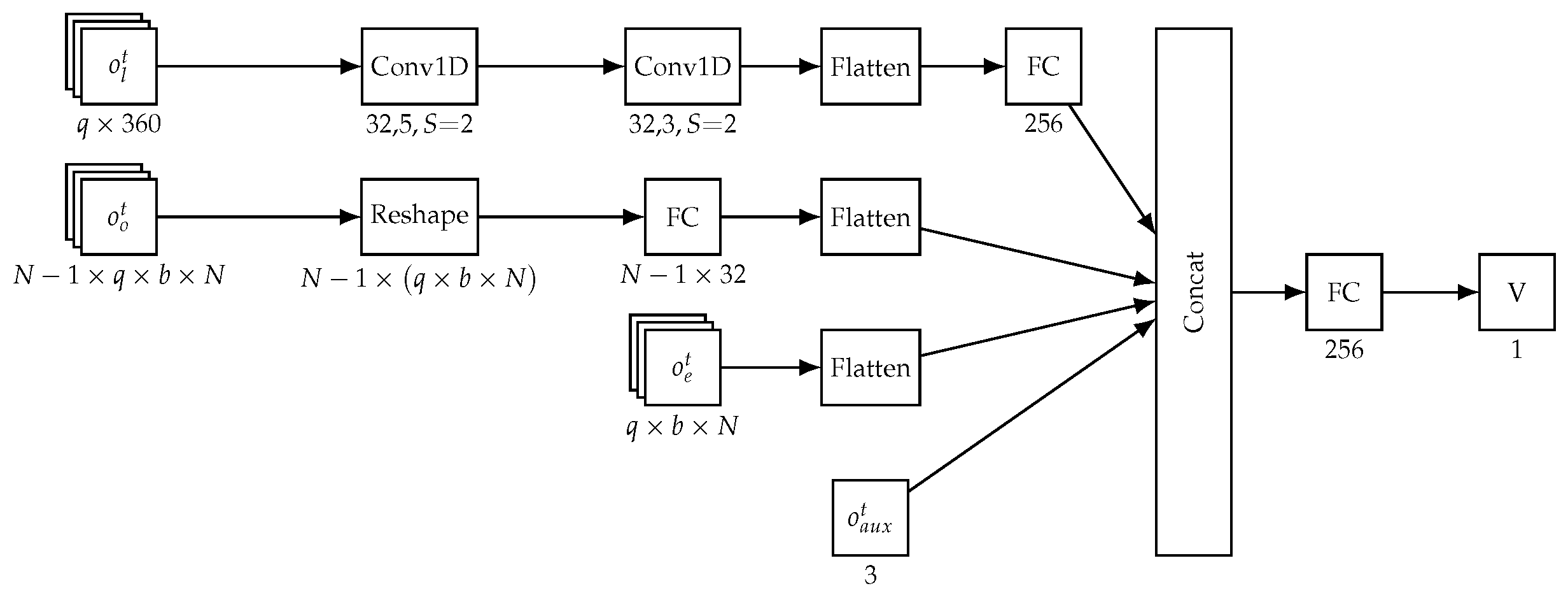
The policy network π θ takes the observation O i t as the input and outputs the action a i t . Figure 1 shows the architecture of the policy network. There are four inputs to the policy network, and each one corresponds to one of the observation components O i t = o e t , o o t , o l t , o a u x t , while each input has its branch of hidden layers through which it passes. The input o l t goes through the first branch, and it passes through a convolutional layer [20] that consists of 32 one-dimensional filters with a kernel size of 5 and a stride of 2, the second hidden layer in the branch is a another convolutional layer similar to the first one, except it has a kernel size of 3. The third hidden layer is a flatten layer followed by a 128 neuron fully-connected layer [20]. The second branch that takes input o o t passes it through a reshape layer that reshapes it into the shape R N 1 × q × b × N , then it is passed through a 32 neuron fully-connected layer applied on the last dimension of the reshape layer output, and then, the output of the fully connected layer is flattened. The observation o e t goes through the third branch, which is just one flatten layer. The fourth branch has no hidden layers; it passes the o a u x t input through to the next stage. The outputs of all the branches are then concatenated, then passed through a 256 neuron fully-connected layer. All the layers until now have ReLU activations [21]. The final layers are the two output layers, each corresponding to an action component a i t = v l t , v r t , and each layer has K neurons with softmax activations [22]. The components of the action a i t are then sampled from the two softmax distributions, as explained in Section 4.1.2.
The value network V ϕ shown in Figure 2 shares the same architecture as the policy network except for the outputs. The output layer of the value network outputs the network’s prediction of the value estimation, and it is a single neuron fully-connected layer with no activations. The value network has a separate set of weights with respect to the policy network.

5. Experiments and Results

5.1. Simulation Environment

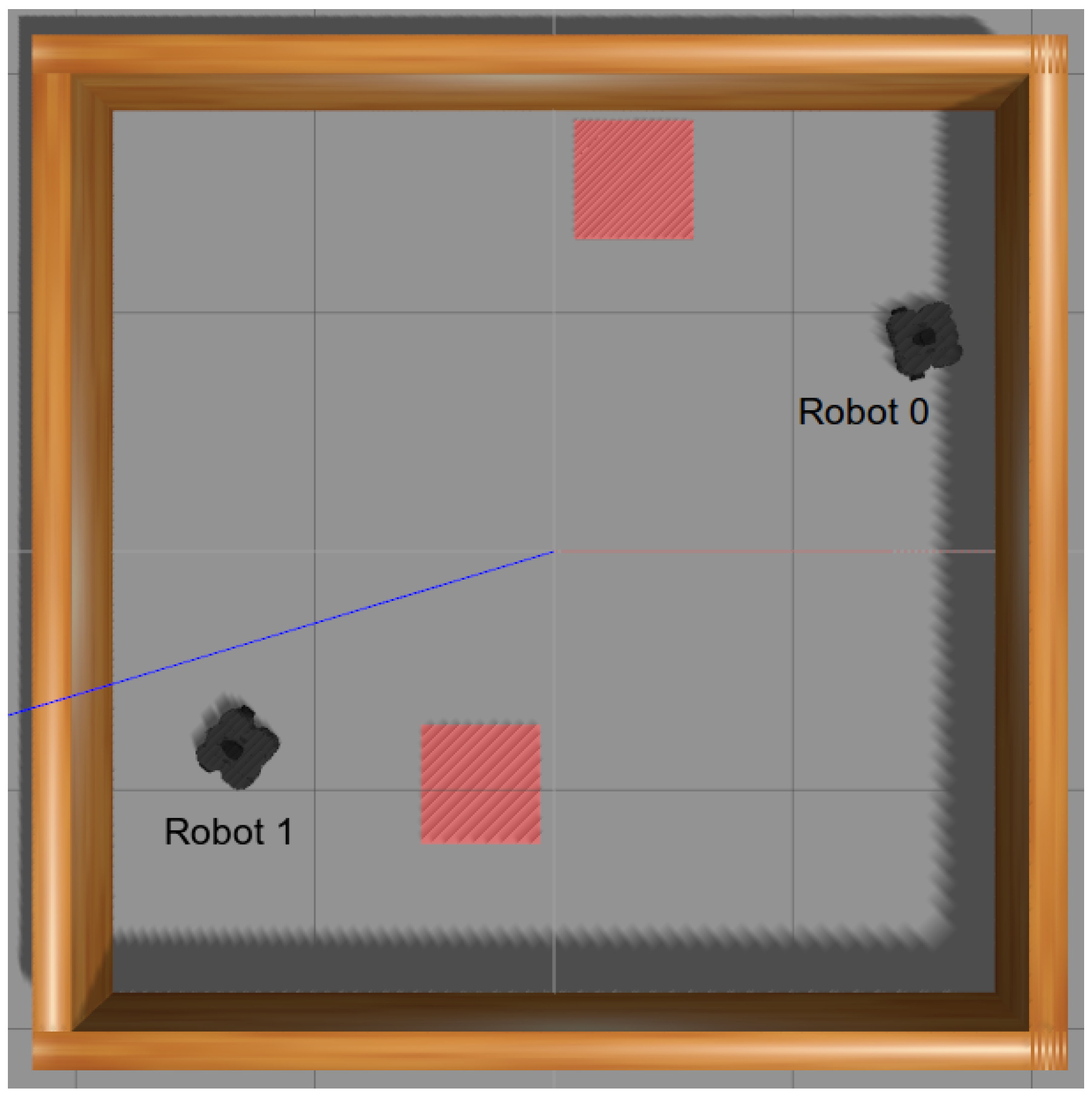
We developed a simulation environment to train and test our deep reinforcement learning method. The robots used were the Turtlebot3 Waffle PI robots [23]. We adapted the simulation environment built by the Turtlebot3 robot team and modified the environment to support multiple robots and goal positions. The simulation environment was built using the Gazebo simulator [24], as shown in Figure 3. The simulation environment was a 4 m × 4 m square environment surrounded by a fence. The robots and the goal positions were spawned inside the environment. The robots had fixed starting positions, while the goals’ positions were chosen randomly from a set of predefined positions. In the case of training, the set of predefined goals positions held 33 positions, while during testing, it held the same goal positions with 10 extra positions to test for generality. The goal positions were changed when each robot reached a unique goal successfully or when a certain amount of episodes E g had passed since the last goal positions changed.
During training, ten simulation environments were launched in parallel. Each of them contained two robots N = 2 with a total of 20 robots. Each of the robots had a copy of the policy and value networks and used them for data collection. After the data were collected, the data were sent to a centralized copy of the policy and value networks to be updated. Then, the updated weights were sent back to each copy.

5.2. Training Configuration

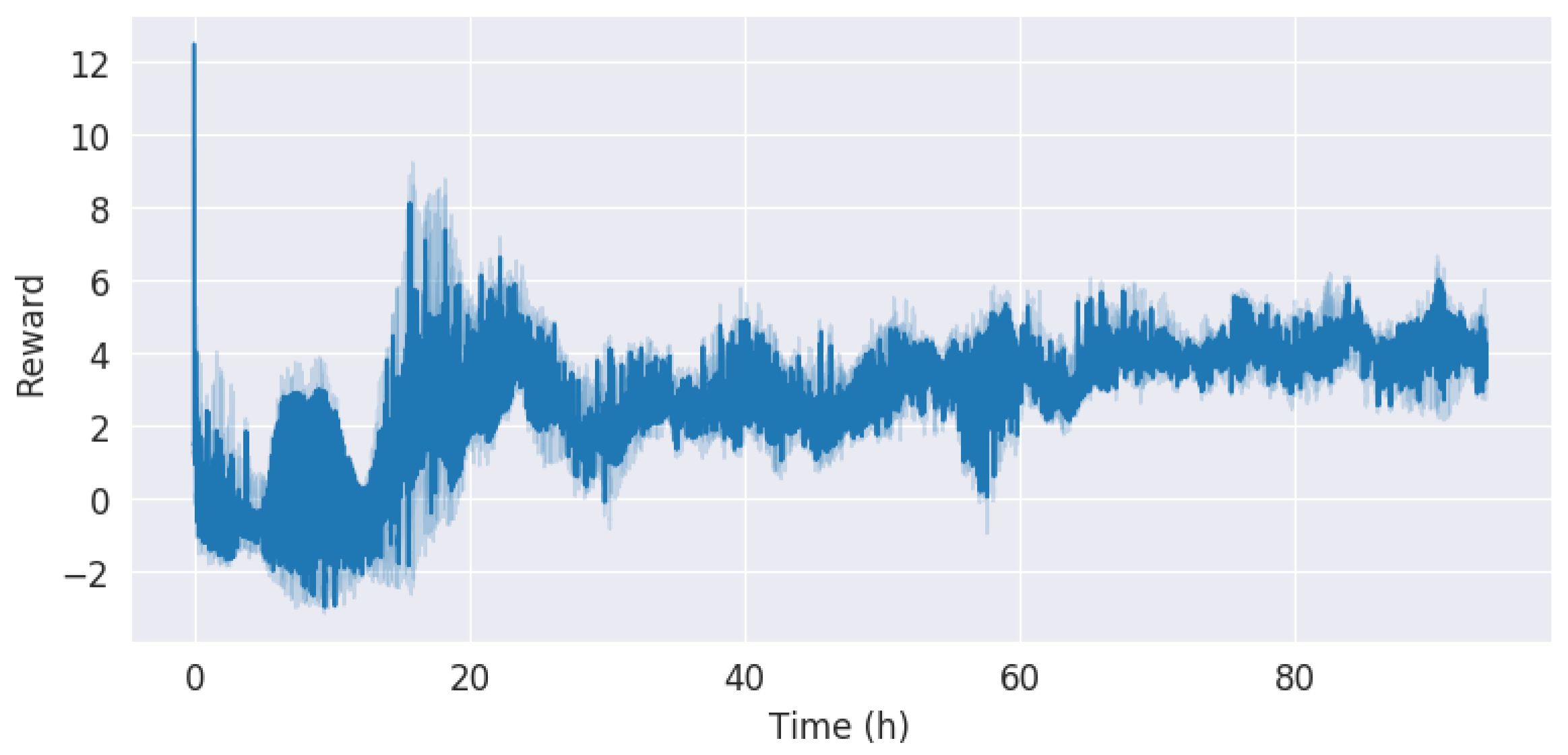
The algorithm was implemented using TensorFlow [25] on an NVIDIA DGX-1 station. The training took 94 h (about 8 k iterations). The frequency of computing the actions on which the policy was operating was set to 5 Hz. Table 2 shows the hyperparameters used during training. The evolution of the reward over training is shown in Figure 4.

5.3. Evaluation and Testing

The overall performance of the policy can be evaluated using the same quantitative metrics used by Long et al. [12]:
  • Success rate: The ratio of the number of robots that reach unique goals successfully during the episode over the total number of robots (the higher the better).
  • Extra time: The difference between the actual travel time of a robot to reach a goal position and the time it takes the robot to go to the same goal position in a straight line with maximum speed (the lower the better).
  • Extra distance: The difference between the actual distance a robot traveled to reach a goal position and the Euclidean distance between the robot’s start position and the goal position (the lower the better).
  • Average speed: The average of the ratio of the speed of the robot team relative to the maximum speed of a robot during the episode.
The metrics were measured over all the robots and all episodes during the evaluation to remove any effects of the variance in the goals’ positions.
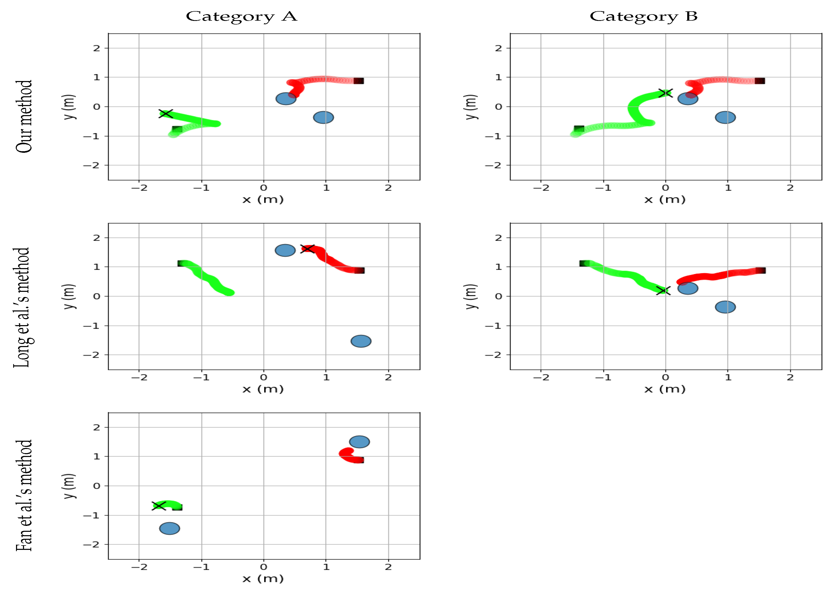
We categorized the robot collisions into three categories. Category A is a collision with an obstacle; Category B is one robot colliding with another robot that reached a goal position; and finally, Category C is two robots colliding together while moving in free space. These three categories cover 100 % of the collision events that might happen in our setting. This categorization can be used to analyze the policy’s performance when it fails and what kinds of collisions tend to happen. Such an analysis can give us insight into the behavior that the policy was trained to perform.
As our method combines MRTA and navigation, the categorization of collisions enabled us to develop a new metric that can measure the performance of our method and future methods that will be similar to it in performing MRTA. This metric can measure the MRTA performance by measuring the policy’s failure in performing MRTA. We call this new metric the Task Allocation Index T A I . It depends on the ratio of episodes ending with Category B collisions relative to the total number of episodes because Category B collisions are a clear failure of MRTA when two robots reach the same goal. T A I also depends on the ratio of goals whose information is input to the policy relative to the total number of goals in the environment, as this gives a higher score for the policies that perform task allocation on a bigger ratio of goals that are available in the environment. Equation (14) shows the formula for T A I (the higher the T A I value the better). For the policies that only perform navigation and do not perform MRTA at all, the T A I value will be zero.
T A I = N i 1 N g 1 × 1 N C a t e g o r y B N E p i s o d e s
where:
  • N i : number of goals whose information is input to the policy.
  • N g : total number of goals.
  • N C a t e g o r y B : number of episodes ended by Category B collisions.
  • N E p i s o d e s : total number of episodes.
We compared our method with the methods proposed by Long et al. [12] and Fan et al. [13]. The reason we are comparing with these works is the similarity in the objective of the studies in terms of performing the navigation of multi-robot systems using deep reinforcement learning. On the other hand, the difference between our method and the methods proposed by Long et al. [12] and Fan et al. [13] is that our policy selects which goal position to drive the robot towards. For the methods of Long et al. [12] and Fan et al. [13], the policy needs the goal position to be preselected per robot. Thus, our method performs MRTA and navigation form end-to-end, while the other methods only perform navigation from end-to-end. The second reason these methods were chosen is because the performance metrics were reported by both papers. Long et al [12] reported better performance than the NH-ORCAmethod over most test cases. We trained the method proposed by Long et al [12] on our simulation setup with the same robot kind we are using. Their method was implemented using the same setup, network architecture, and hyperparameters that they proposed in their paper. The training process took around 22 h. For the method proposed by Fan et al. [13], we used the same policy that we trained for Long et al.’s [12] method as part of the hybrid control system similar to what Fan et al. [13] did in their paper.
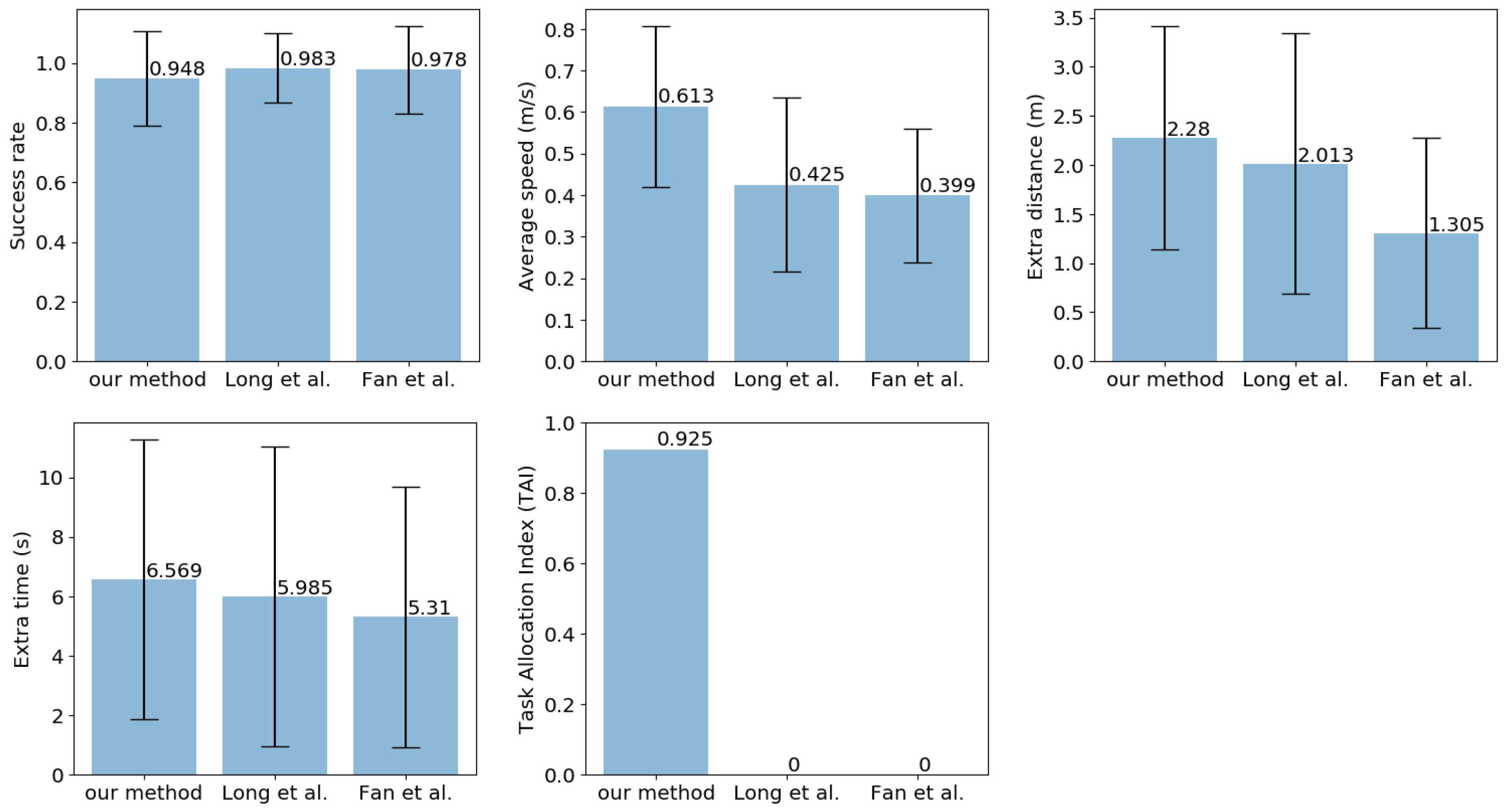
To test and evaluate each method, we repeated the evaluations for 2 h. The goals’ positions were changed every time each robot reached a unique goal or five episodes passed by since the last goal position change E g = 5 . The results are shown in Figure 5. It shows that both methods are on par with each other with a slight advantage of the method proposed by Long et al. [12] over both of the other methods in terms of the success rate. In terms of extra tie and extra distance, the method proposed by Fan et al. [13] has an advantage over the other two methods. This advantage is attributed to the PID policy of the hybrid control system, which drives the robot directly toward the goal position if there is no obstacle nearby or the goal position is closer to the robot than the nearest obstacle. On the other hand, the T A I metric highlights the advantages of our method over the other two methods since our method is the only one that performs both MRTA and navigation from end-to-end. Our method takes input information about all the goals in the environment ( N i = N g in Equation (14)); thus, the only factor affecting the value of the T A I metric in this case is the percentage of episodes ending with Category B collisions N C a t e g o r y B , as shown in Table 3. On the other hand, the T A I metric for both Long et al.’s [12] and Fan et al.’s [13] methods is zero since both methods do not perform MRTA, and they only have input information about the preassigned goal position for each robot ( N i = 1 ).
Table 3 shows the statistics related to the number of episodes and the way they ended for each method. Both methods have a very low percentage of episodes ending with collisions, yet Fan et al.’s [13] method has a slight advantage. We attribute our method’s performance to our method’s tendency to move the robots with an average speed that is higher than the average speed produced by the other methods—as shown in Figure 5—which can lead to the robots in our method having more collisions.
Table 3 also shows the percentage of the occurrence of each collision category during testing. It shows that all methods managed to avoid any collisions of Category C. Our method tends to have collisions of Category B about five times more than that of Category A, which indicates that the policies on both robots chose the same goal position to move towards. Samples of both categories of collisions are visualized in Figure 6.
On the other hand, Long et al.’s [12] method tends to have slightly more collisions of Category A than that of Category B. Most of the Category A collisions occur when the goal position is near the obstacle wall, which means that the policy drives the robot to approach such goals at an angle that exposes it to collision. Alternatively, the Category B collisions occur when the other robot reaches a goal position that is in the middle between the ego-robot and its assigned goal position, as shown in Figure 6, which indicates that the policy failed to avoid a stationary robot in front of it. As for Fan et al.’s [13] method, the only instance when a collision occurred was when a certain goal configuration appeared during testing. This collision instance is Category A, as shown in Figure 6. This collision happens when a goal position is spawned behind Robot 1 and the conservative safe policy of Fan et al.’s [13] hybrid control system is the policy controlling the robot.
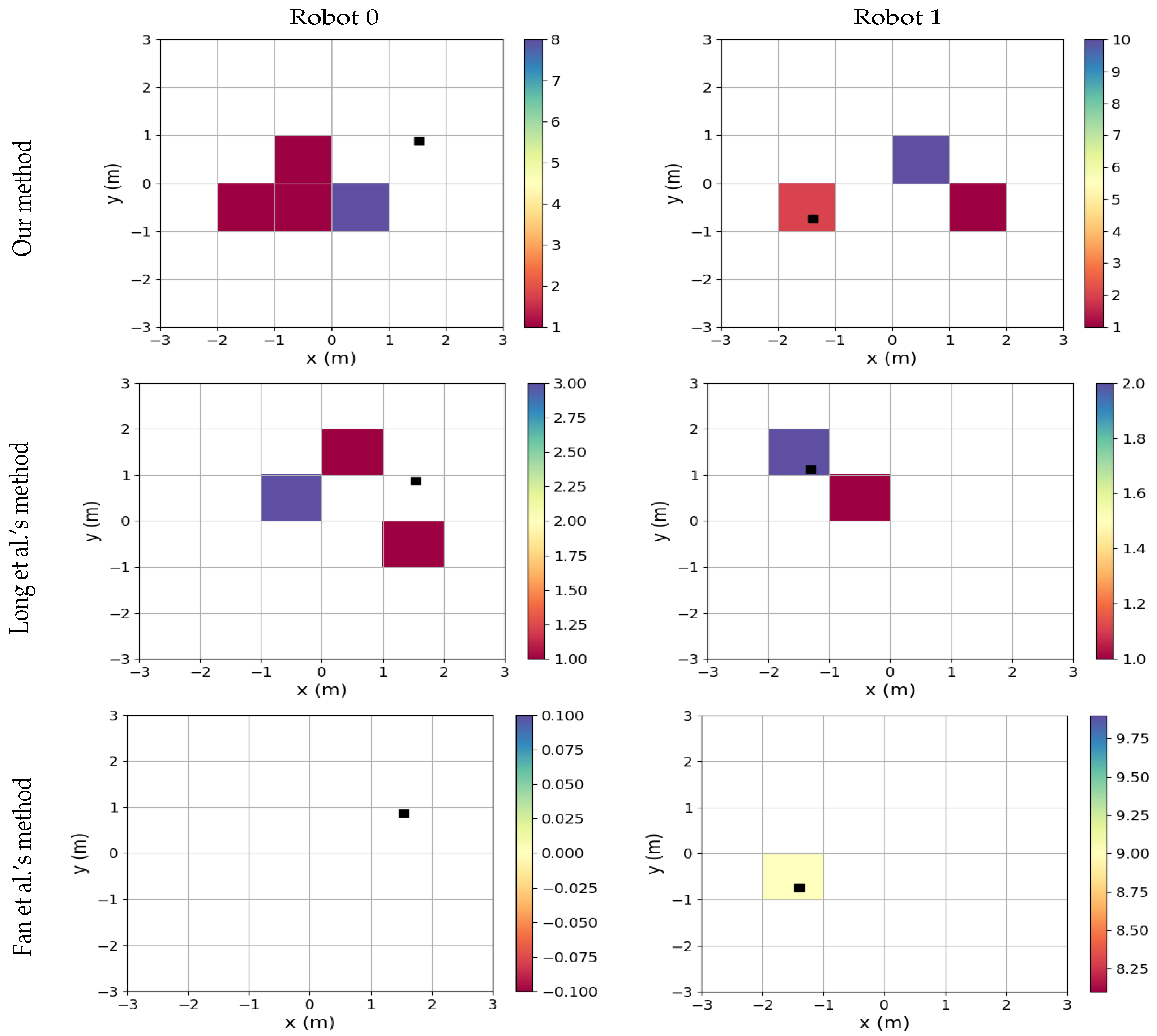
Figure 7 shows the distribution of collisions within the environment. The figure reinforces the analysis of both Table 3 and Figure 6 as it shows that for our method, the collisions are concentrated in the middle of the environment and such collisions are Category B. On the other hand, for Long et al.’s [12] method, most collisions are near the edges of the environment, and such collisions are Category A. For Fan et al.’s [13] method, the collisions only occur for Robot 1 at the same position, and this collision is Category A.
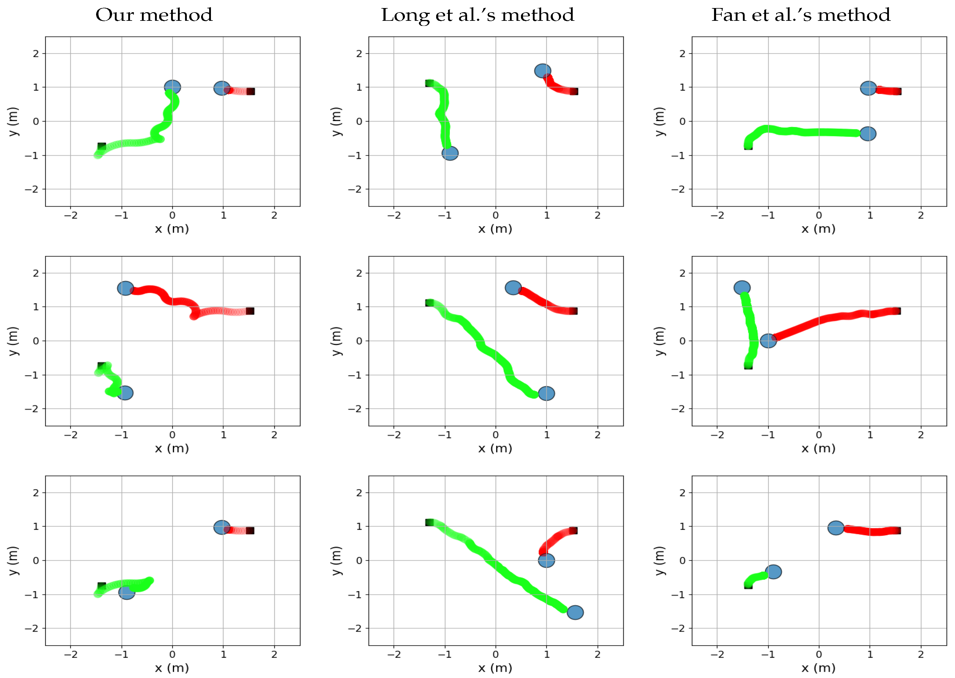
In Figure 8, we visualize three different successful episodes from testing for each method. the visualization shows the trajectory of each robot color coded. It is clear form the graph that the methods of Long et al. [12] and Fan et al. [13] tend to move the robots in more straight trajectories, while our method tends to move in trajectories that are more irregular and sometimes overshoots the goal positions.
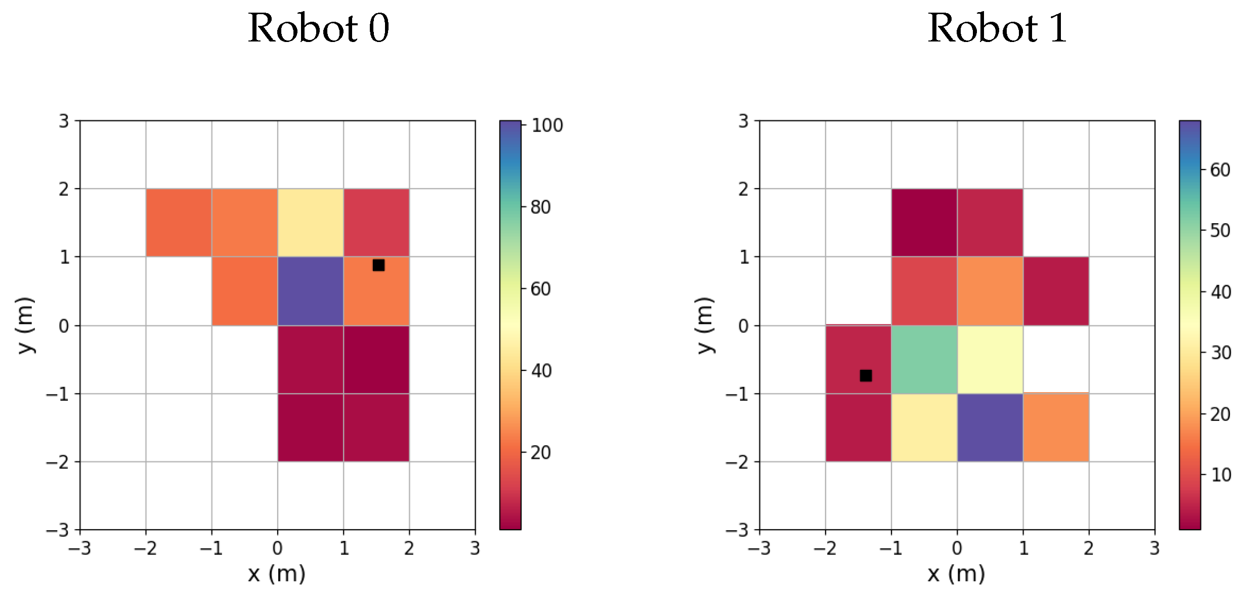
Figure 9 shows the distribution of goals reached by each robot throughout the environment during testing for our method. It shows that Robot 0, which is spawned near the upper right corner of the environment, tends to reach the goals positioned in the environment’s upper half, while Robot 1, which is spawned in the lower left corner, tends to reach the goals positioned in the environment’s lower half. The past two observations indicate that the task allocation strategy learned during training is to split the environment into two halves, and each robot attempts to reach the goals available in its half.
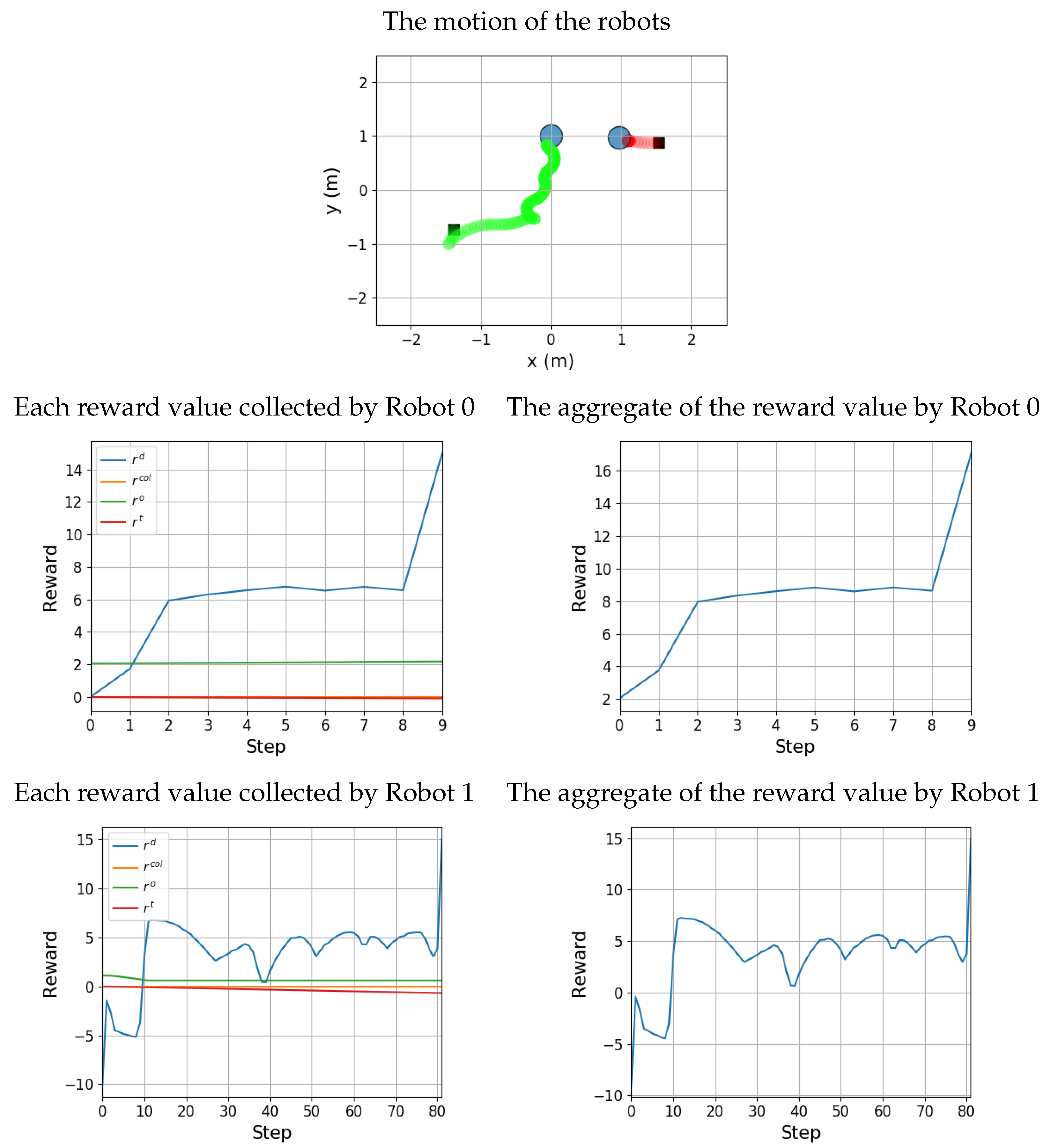
To analyze the reward function for our method that was introduced in Section 4.1.3 and to evaluate the effects of the values of the constants for the reward function that are shown in Table 2, Figure 10 and Figure 11 visualize the reward function during a successful episode and an episode that ended with a collision, both episodes by our method. For the successful episode in Figure 10, the reward r d —described in Equation (7)—which is used to incentivize the ego-robot to go towards a goal position, has a positive value for both robots as each of them goes towards the goal position and has a large terminal value once each robot reaches a unique goal position. An exception to that happened at the beginning of the episode for Robot 1 since the policy moved it away from the goal position for the first 10 time steps. As for the other reward functions, since there were no collisions, therefore the reward r c o l —described in Equation (10)—had a zero value for both robots. Since no robot went towards the same goal position as the other robot, the reward function r o —described in Equation (12)—had a positive value for both robots. As for the reward function r t —described in Equation (13)–it had a very small negative value for Robot 0 as it took the robot 2.22 s to reach its goal position. On the other hand, Robot 1 had a slightly lower r t reward as it took 16.93 s to reach its goal position.
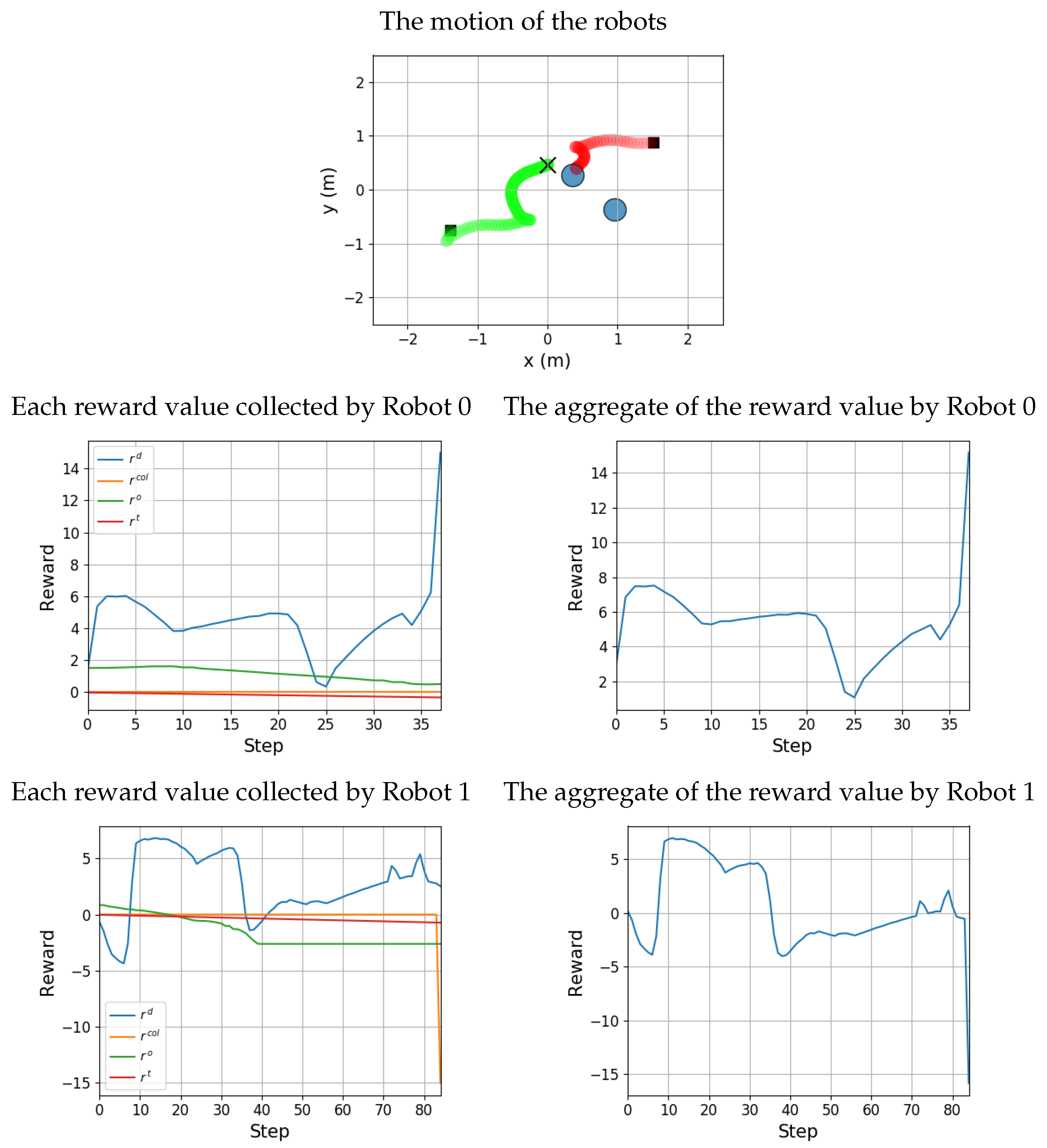
On the other hand, the episode that ended in a collision is shown in Figure 11. The collision that occurred in this episode is Category B. Since Robot 0 reached a goal position successfully, therefore its aggregate reward function showed positive values across its movement, and when the robot reached the goal position, a large terminal reward value was given to the robot. On the other hand, Robot 1 moved towards the same goal position as Robot 0 and collided with it. This behavior is reflected in the reward function as the reward function r o —described in Equation (12)—took on a negative value once Robot 1 started to move towards the same goal position as Robot 0. Once the collision occurred, Robot 1 received a large negative terminal reward according to the reward r c o l —described in Equation (10). The combination of all of the rewards led to the aggregate reward received by Robot 1 having a negative value for most of the time steps.

6. Conclusions

In this paper, we present a novel decentralized sensor level policy that performs multi-robot task allocation and navigation from end-to-end. We train and test it in a simulation environment using a simulation of a real robotic platform. We also propose a new metric called the Task Allocation Index ( T A I ), which measures the performance of a method that performs MRTA and navigation from end-to-end in performing MRTA. Our method is compared with two other DRL based methods that only perform navigation for a multi-robot system. Our method shows on par results compared to these methods with a slight advantage for the other methods in terms of the success rate, extra time, and extra distance. On the other hand, our method outperforms the other two methods in terms of the Task Allocation Index ( T A I ) as the two other methods do not perform MRTA. Our work serves as a starting point towards building a robust system that performs task allocation and navigation from end-to-end. Future works include training our method on more complex environments and experimental setups to validate our method. We also plan in the future to use some more advanced network architectures to increase the performance and to adapt some of the methods used in natural language processing to allow the neural network architecture to accept observations with a variable number of robots in the system.

Author Contributions

Supervision, Z.H.I.; conceptualization, software, and writing, A.E. All authors read and agreed to the published version of the manuscript.

Funding

This research work was funded by the Ministry of Higher Education Malaysia and Universiti Teknologi Malaysia under FRGS Grant no. R.K130000.7843.5F348.

Conflicts of Interest

The authors declare no conflict of interest.

References

  1. Gerkey, B.P.; Matarić, M.J. A formal analysis and taxonomy of task allocation in multi-robot systems. Int. J. Robot. Res. 2004, 23, 939–954. [Google Scholar] [CrossRef] [Green Version]
  2. Yu, J.; LaValle, S.M. Optimal Multirobot Path Planning on Graphs: Complete Algorithms and Effective Heuristics. IEEE Trans. Robot. 2016, 32, 1163–1177. [Google Scholar] [CrossRef]
  3. Woosley, B.; Dasgupta, P. Multirobot Task Allocation with Real-Time Path Planning. In Proceedings of the Twenty-Sixth International Florida Artificial Intelligence Research Society Conference, St. Pete Beach, FL, USA, 22–24 May 2013; pp. 574–579. [Google Scholar]
  4. Sutton, R.S.; Barto, A.G. Reinforcement Learning: An Introduction, 2nd ed.; The MIT Press: Cambridge, MA, USA, 2018. [Google Scholar]
  5. Arulkumaran, K.; Deisenroth, M.P.; Brundage, M.; Bharath, A.A. A Brief Survey of Deep Reinforcement Learning. IEEE Signal Process. Mag. 2017, 34, 26–38. [Google Scholar] [CrossRef] [Green Version]
  6. Nguyen, T.T.; Nguyen, N.D.; Nahavandi, S. Deep Reinforcement Learning for Multiagent Systems: A Review of Challenges, Solutions, and Applications. IEEE Trans. Cybern. 2020, 50, 3826–3839. [Google Scholar] [CrossRef] [Green Version]
  7. Buşoniu, L.; de Bruin, T.; Tolić, D.; Kober, J.; Palunko, I. Reinforcement learning for control: Performance, stability, and deep approximators. Annu. Rev. Control. 2018, 46, 8–28. [Google Scholar] [CrossRef]
  8. Zhu, Q.; Oh, J. Deep Reinforcement Learning for Fairness in Distributed Robotic Multi-type Resource Allocation. In Proceedings of the 17th IEEE International Conference on Machine Learning and Applications, ICMLA, Orlando, FL, USA, 17–20 December 2018; pp. 460–466. [Google Scholar] [CrossRef]
  9. Dai, W.; Lu, H.; Xiao, J.; Zeng, Z.; Zheng, Z. Multi-Robot Dynamic Task Allocation for Exploration and Destruction. J. Intell. Robot. Syst. Theory Appl. 2019, 1–25. [Google Scholar] [CrossRef]
  10. Chen, Y.F.; Liu, M.; Everett, M.; How, J.P. Decentralized non-communicating multiagent collision avoidance with deep reinforcement learning. In Proceedings of the IEEE International Conference on Robotics and Automation, Singapore, 29 May–3 June 2017; pp. 285–292. [Google Scholar]
  11. Lin, J.; Yang, X.; Zheng, P.; Cheng, H. End-to-end Decentralized Multi-robot Navigation in Unknown Complex Environments via Deep Reinforcement Learning. In Proceedings of the IEEE International Conference on Mechatronics and Automation (ICMA); Institute of Electrical and Electronics Engineers (IEEE): Tianjin, China, 2019; pp. 2493–2500. [Google Scholar] [CrossRef] [Green Version]
  12. Long, P.; Fan, T.; Liao, X.; Liu, W.; Zhang, H.; Pan, J. Towards Optimally Decentralized Multi-Robot Collision Avoidance via Deep Reinforcement Learning. In Proceedings of the 2018 IEEE International Conference on Robotics and Automation (ICRA), Brisbane, Australia, 21–25 May 2018; pp. 6252–6259. [Google Scholar] [CrossRef] [Green Version]
  13. Fan, T.; Long, P.; Liu, W.; Pan, J. Distributed multi-robot collision avoidance via deep reinforcement learning for navigation in complex scenarios. Int. J. Robot. Res. 2020, 39, 856–892. [Google Scholar] [CrossRef]
  14. Mnih, V.; Kavukcuoglu, K.; Silver, D.; Rusu, A.A.; Veness, J.; Bellemare, M.G.; Graves, A.; Riedmiller, M.; Fidjeland, A.K.; Ostrovski, G.; et al. Hum. Level Control. Deep. Reinf. Learn. Nature 2015, 518, 529–533. [Google Scholar] [CrossRef] [PubMed]
  15. Van Den Berg, J.; Guy, S.J.; Lin, M.; Manocha, D. Reciprocal n-body collision avoidance. In Springer Tracts in Advanced Robotics; Springer: Berlin/Heidelberg, Germany, 2011; Volume 70, pp. 3–19. [Google Scholar] [CrossRef]
  16. Schulman, J.; Wolski, F.; Dhariwal, P.; Radford, A.; Openai, O.K.; Klimov, O. Proximal Policy Optimization Algorithms. arXiv 2017, arXiv:1707.06347. [Google Scholar]
  17. Spaan, M.T.J. Partially Observable Markov Decision Processes. In Reinforcement Learning; Wiering, M., van Otterlo, M., Eds.; Springer: Berlin/Heidelberg, Germany, 2012; Chapter 12; pp. 387–414. [Google Scholar] [CrossRef]
  18. Kingma, D.P.; Ba, J.L. ADAM: A METHOD FOR STOCHASTIC OPTIMIZATION. In Proceedings of the 3rd International Conference on Learning Representations, ICLR, San Diego, CA, USA, 7–9 May 2015; pp. 1–15. [Google Scholar] [CrossRef]
  19. Schulman, J.; Moritz, P.; Levine, S.; Jordan, M.I.; Abbeel, P. High-Dimensional Continuous Control Using Generalized Advantage Estimation. In Proceedings of the 4th International Conference on Learning Representations (ICLR 2016), San Juan, Puerto Rico, 2–4 May 2016. [Google Scholar]
  20. Lecun, Y.; Bengio, Y.; Hinton, G. Deep learning. Nature 2015, 521, 436–444. [Google Scholar] [CrossRef] [PubMed]
  21. Nair, V.; Hinton, G.E. Rectified Linear Units Improve Restricted Boltzmann Machines. In Proceedings of the 27th International Conference on Machine Learning, Haifa, Israel, 21–24 June 2010; pp. 807–814. [Google Scholar]
  22. Martins, A.; Astudillo, R. From softmax to sparsemax: A sparse model of attention and multi-label classification. In Proceedings of the 33rd International Conference on Machine Learning, New York, NY, USA, 19–24 June 2016; Volume 48, pp. 1614–1623. [Google Scholar]
  23. Kim, A.; Seon, D.; Lim, D.; Cho, H.; Jin, J.; Jung, L.; Will Son, M.Y.; Pyo, Y. TurtleBot3 e-Manual. Available online: http://emanual.robotis.com/docs/en/platform/turtlebot3/overview/ (accessed on 15 March 2020).
  24. Koenig, N.; Howard, A. Design and use paradigms for Gazebo, an open-source multi-robot simulator. In Proceedings of the 2004 IEEE/RSJ International Conference on Intelligent Robots and Systems (IROS), Sendai, Japan, 28 September–2 October 2004; Volume 3, pp. 2149–2154. [Google Scholar] [CrossRef] [Green Version]
  25. Abadi, M.; Barham, P.; Chen, J.; Chen, Z.; Davis, A.; Dean, J.; Devin, M.; Ghemawat, S.; Irving, G.; Isard, M.; et al. TensorFlow: A System for Large-Scale Machine Learning TensorFlow: A system for large-scale machine learning. In Proceedings of the 12th USENIX Symposium on Operating Systems Design and Implementation (OSDI ’16), Savannah, GA, USA, 2–4 November 2016; pp. 265–283. [Google Scholar]
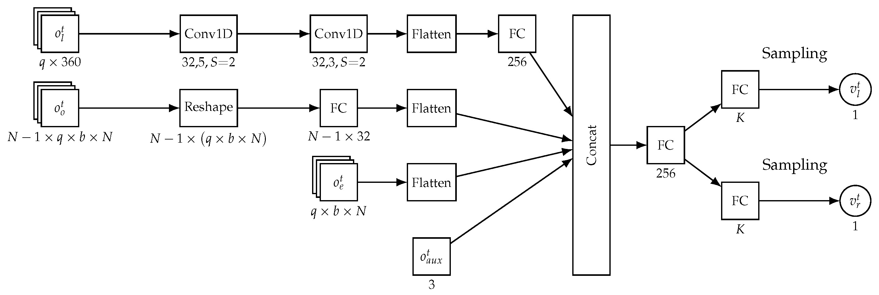
Figure 1. Policy network architecture.
Applsci 11 02895 g001
Figure 2. Value network architecture.
Applsci 11 02895 g002
Figure 3. The simulation environment. The size of the environment is 4 m × 4 m, and it is shown holding two robots with two goal positions.
Applsci 11 02895 g003
Figure 4. Average of the rewards gained per episode averaged over all the robots in the training wall time.
Applsci 11 02895 g004
Figure 5. The performance results of each method during a 2 h test.
Applsci 11 02895 g005
Figure 6. The trajectories of the robots over three different episodes that ended by collisions during testing performed by each method. The trajectory of Robot 0 is shown in red, while the trajectory of Robot 1 is shown in green. The more opaque the color of the trajectory is, the more advanced in time it is. The environment spans the interval [−2, 2] for both the x and y axes. The black squares represent the starting positions of the robots; the blue circles represent the goal positions, and the “×” shape represents the collisions’ locations.
Applsci 11 02895 g006
Figure 7. The distribution of collisions in the environment done by each robot controlled by each method during testing. The environment spans the interval [−2,2] for both the x and y axes. The black squares represent the starting positions of the robots.
Applsci 11 02895 g007
Figure 8. The trajectories of the robots over three different episodes that ended successfully during testing performed by both methods. The trajectory of Robot 0 is shown in red, while the trajectory of Robot 1 is shown in green. The more opaque the color of the trajectory is, the more advanced in time it is. The environment spans the interval [−2,2] for both the x and y axes. The black squares represent the starting positions of the robots, and the blue circles represent the goal positions.
Applsci 11 02895 g008
Figure 9. The distribution of the reached goal positions in the environment done by each robot controlled by our method during testing. The environment spans the interval [−2,2] for both the x and y axes. The black squares represent the starting positions of the robots.
Applsci 11 02895 g009
Figure 10. Visualizing the rewards collected by each robot using our method in an episode that ended successfully. The trajectory of Robot 0 is shown in red, while the trajectory of Robot 1 is shown in green.
Applsci 11 02895 g010
Figure 11. Visualizing the rewards collected by each robot using our method in an episode that ended with a collision. The trajectory of Robot 0 is shown in red, while the trajectory of Robot 1 is shown in green.
Applsci 11 02895 g011
Table 1. The summary of the presented works from the literature that either perform multi-robot task allocation (MRTA) or navigation using DRL.
PaperMRTANavigation
Zhu et al. [8]X
Chen et al. [10]X
Lin et al. [11]X
Long et al. [12]X
Fan et al. [13]X
Our proposed method
Table 2. The hyperparameters and constants used for training. GAE, generalized advantage function.
ParameterDescriptionValue
qNumber of consecutive frames used in each observation5
T t h Data collection threshold1100
λ GAE decay factor0.92
γ Discount factor0.98
T m a x Max. episode time120 s
ENumber of epochs10
ϵ Used in the surrogate objective function0.2
c 1 The value loss factor5.0
c 2 The entropy loss factor0.01
l r Learning rate5 × 10−5
E g Number of episodes to change the goal positions50
T m a x Max. episode time120 s
r t e r m i n a l Terminal reward15
w g Goal’s distance factor200
w o t h 1 Occupied goal reward Factor 13.5
w o t h 2 Occupied goal reward Factor 23.409
w t Time reward factor−5
RRobot radius0.2 m
Table 3. Performance metrics for both methods during a 2 h test.
MetricOur MethodLong et al.Fan et al.
Number of episodes268402425
% of episodes ending by collision8.955%2.239%2.118%
% of episodes ending by Category A collision1.522%1.254%2.118%
% of episodes ending by Category B collision7.433%0.985%0.0%
% of episodes ending by Category C collision0.0%0.0%0.0%
% of episodes ending by exhausting episode time0.746%0.0%0.0%
Publisher’s Note: MDPI stays neutral with regard to jurisdictional claims in published maps and institutional affiliations.