Abstract
Sound absorbing micro-perforated panels (MPPs) are being increasingly used because of their high quality in terms of hygiene, sustainability and durability. The present work investigates the feasibility and the performance of MPPs when used as an acoustic treatment in lecture rooms. With this purpose, three different micro-perforated steel specimens were first designed following existing predictive models and then physically manufactured through 3D additive metal printing. The specimens’ acoustic behavior was analyzed with experimental measurements in single-layer and double-layer configurations. Then, the investigation was focused on the application of double-layer MPPs to the ceiling of an existing university lecture hall to enhance speech intelligibility. Numerical simulations were carried out using a full-spectrum wave-based method: a finite-difference time-domain (FDTD) code was chosen to better handle time-dependent signals as the verbal communication. The present work proposes a workflow to explore the suitability of a specific material to speech requirements. The measured specific impedance complex values allowed to derive the input data referred to MPPs in FDTD simulations. The outcomes of the process show the influence of the acoustic treatment in terms of reverberation time () and sound clarity (). A systematic comparison with a standard geometrical acoustic (GA) technique is reported as well.
1. Introduction
Nowadays, the interest in sound absorbing materials is growing due to the variety of their possible applications, from room acoustics [1] to environmental noise control [2,3]. Porous and fibrous absorbers [4,5,6] have until now been the most used materials in noise control application because of their high performance-to-cost ratio in the frequency band of interest. In the last decades, new requirements have become important, such as durability, recyclability, hygienic problems, environmental sustainability and optical transparency, which are no longer suitable for porous and fibrous materials. In order to satisfy these requirements, specific classes of sound absorbing materials have been proposed: among them, micro-perforated panels (MPPs) [7,8,9,10,11]. During the 1970s, the first MPP acoustic model proposed by Maa [7] defined the absorbers as a combination of a thin panel with sub-millimetric holes, an air cavity and a rigid wall. The air cavity is required to perform a Helmholtz-type resonance. Moreover, an equivalent fluid (EF) model was theorized by Atalla and Sgard [12]. In the last decades, the applications, the improvements and the theoretical developments of such materials have been extensively studied and MPP multiple-layers have been introduced to provide wide-band absorption, creating more efficient sound absorbing systems [13,14,15].
MPPs can be made of various materials, including plywood, glass and sheet metal. Therefore, they are extremely attractive from an ecological point of view, especially for architectural applications [16,17]. Among the potential applications of MPPs, there is their use as an acoustic treatment in existing lecture rooms to enhance the verbal communication conditions [18]. Reducing the reverberant field in a specific frequency range contributes to decreasing the vocal effort of the speaker and the distraction of the students [19,20,21]. Since in the last years the acoustical comfort of teachers and students is one of the most debated topics [22,23,24], the possibility to choose a sustainable and high-performance material could meet the need of improving the acoustics in existing lecture halls.
In this work, three steel MPP specimens were designed with specific constitutive geometrical parameters. The sound absorption mathematical equations and the electro-acoustic analogies were used to simplify complex mechanical issues into equivalent electrical circuits. The specimens were constructed using 3D additive printing and the manufacturing issues encountered during the process are described and shown in detail. Experimental measurements made with the transfer-function method [25] in an impedance tube [26] are reported and compared with predictive models. An optimization of MATLAB implementations was carried out taking into account the practical issues encountered during the measurements. After the experimental phase, the performance of MPPs was evaluated focusing on the application to large-scale rooms. In particular, the effects of MPPs as an acoustic treatment in an existing lecture hall previously surveyed [27] were explored by means of full-spectrum finite-difference time-domain (FDTD) simulations [28].
2. Modeling the Sound Absorption of Micro-Perforated Panels (MPP)
A micro-perforated panel consists of a thin panel with a specific perforation ratio made by a distribution of sub-millimeter holes backed by an air cavity and a rigid wall, as shown in Figure 1.
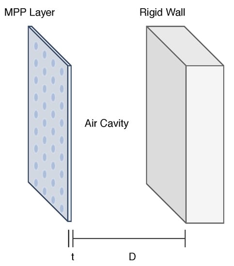
Figure 1.
Schematic representation of a single-layer micro-perforated panel (MPP) and its dimensional parameters.
The acoustic complex impedance of an MPP (Z) is the result of different contributions: the real part of the impedance that needs to be matched to the air impedance () and the imaginary part of the impedance provided by the air cavity and the perforations. The values of the perforation diameter d, the thickness of the panel t, the porosity and the air cavity thickness D are the four constitutive parameters that influence the range of frequencies absorbed and the bandwidth as well. Taking into account Maa’s definition [8] and according to Cobo’s notation [13], it is possible to define the input complex impedance of a single-layer (SL) MPP as follows:
The impedance defines the viscous dissipation within the holes, the distortion of the flow in the perforation edges and is the resonance in the air cavity:
where is the pressure difference at both sides of the tubes, u is the particle velocity in the tube, is the air density, is the air dynamic viscosity, is the porosity, is the perforation constant (d being the diameter of the holes), and the Bessel functions of first-class and order 1 and 0, respectively, and is the Fok function, a correction factor of the mass reactance [13] and . Considering all the parameters introduced so far, it is possible to study the equivalent electro-acoustic system for the MPP, as shown in Figure 2.
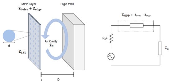
Figure 2.
Single-layer (SL)-MPP schematic representation (left) and the corresponding equivalent electrical system (right).
In practice, multiple-layer MPPs are usually preferred because of their extended absorption band.
A double-layer MPP (DL-MPP) consists of two MPPs with impedances and and two air cavities with impedances and (see Figure 3). Considering the sound waves passing through the DL-MPP system from left to right at normal incidence, the input impedance to the DL-MPP system is:
with
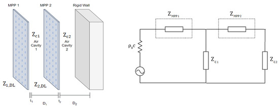
Figure 3.
Double-layer (DL)-MPP schematic representation (left) and the corresponding equivalent electrical system (right).
Therefore, the absorption of a DL-MPP globally depends on eight constitutive and geometrical parameters, four for the first layer and four for the second layer: the diameter of the holes (, ), the thickness (, ), the distance (, ), and the porosity (, ). For this reason, it is difficult to predict the acoustic performance of a DL-MPP and to find, a priori, a combination of these parameters providing the maximum absorption in a specific frequency range.
Atalla and Sgard [12] introduced the so-called equivalent fluid (EF) model following the Johnson–Champoux–Allard approach with an equivalent tortuosity [5]: they assumed an MPP coupled at both sides to a semi-infinite fluid. All of the phenomena involved are recalled in Figure 4. In the EF model, the viscous boundary within the perforations and around the edges is represented by the resistive part of the normal surface impedance, and the movement of the air cylinder—the length of which is greater than the panel thickness—is taken into account in the reactive part of the MPP impedance. In addition to this, a new length correction is introduced in order to consider the increase of air mass vibrating inside the cylinder. Allard demonstrated that the viscous and thermal lengths ( and , respectively) can be considered equal to the hydraulic radius of the perforations in case of straight cylindrical pores.
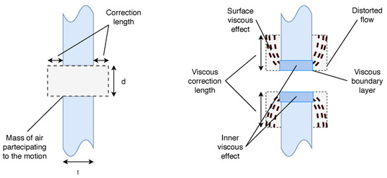
Figure 4.
Physical phenomena involved in an MPP: surface viscous effects and inner viscous effects.
The EF model introduces the effective density , which considers viscous and inertial effects that govern the front face impedance, inside the perforations, defined as:
where is the flow resistivity, defined as . Thus, the impedance of the holes can be rewritten as:
The edge effects are introduced in the EF model through the geometrical tortuosity . In this work, the definition of provided by Atalla and Sgard [12] is used, meaning that not only the intrinsic properties of the material and its micro-geometry but also the media in contact with the panel will be considered. In case of a panel radiating on both sides:
where t is the thickness of the panel, and (valid when ). In the EF model, the tortuosity replaces the Fok function introduced in Maa’s model [9]. Thus, the panel impedance for a SL-MPP using the EF model is:
A double-layer MPP system can be studied with the EF model as well, defining for the second layer of the MPP structure as:
Additionally, as done earlier with the Maa model, the entire double-layer surface impedance is obtained as follows:
3. MPP Samples
The theoretical models have been used as a reference to design and develop different samples of micro-perforated panels. The purpose was to find the best configurations of the double-layer MPP’s parameters in order to predict and simulate the behavior of sound absorbing structures that match the characteristic curve of speech, in view of the application to an university lecture hall.
3.1. Samples Manifacturing
The first step for the realization of an MPP layer was the material choice and, consequently, the standard thickness of the samples. Taking into consideration the sub-millimeter perforation diameter and the high quality standard in terms of durability and endurance, the choice was stainless steel. The aim was to obtain six samples with circular cross-sections and a diameter of ∼40 mm in order to allow the measurements in the impedance tube according to the technical standard ISO 10534-2 [26]. These three types of samples allowed to obtain different combinations between different samples, including double-layer structures with two equal samples. Considering the required perforation size (<1 mm) and geometry (circular cross-section), the stainless steel samples were manufactured using a 3D additive printing technique. A 316L grade stainless steel powder was used, specific for laser powder bed fusion (LPBF). The 3D printing process parameters are reported in Table 1.

Table 1.
3D printing process parameters. LPBF, laser powder bed fusion.
This choice allowed us to print the three different types of samples in a single cylinder of stainless steel with a diameter of ∼40 mm and a height of ∼30 mm as shown in Figure 5, respecting the working restrictions of the printer. Once the stainless steel was printed, the problem was to find a specific cutting technique to make samples of 1 mm thickness. The only possible choice was to use a wire electrical discharge machining (WEDM). The WEDM technique works without increasing the heat during the cutting.
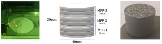
Figure 5.
3D metal printing (left); 3D sketch of the cylinder (center) and real photograph (right) of the cylinder. Two equal samples for three different kinds of specimen were obtained from the cylinder.
Thanks to this technique, two samples of each type were obtained from the cylinder. The thickness of each sample was respected with a tolerance of 0.3–0.6 mm, as shown in Figure 6.
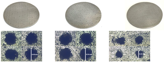
Figure 6.
The three MPP samples (top) and the effective visualisation of perforations seen at the microscope (bottom).
Considering the scale of the perforation size, the real shapes of the perforations were not as expected and the real dimensions were bigger than expected: this was due to the limited accuracy of the processing and manufacturing machinery. Thus, all of the resulting perforations had irregular cross-sections: Ning et al. [29] demonstrated that increasing the specific surface area of a perforation could increase the sound energy dissipation and expand the sound absorption bandwidth, when the inscribed and circumscribed circle are assumed to be unchanged. In fact, keeping constant the outer diameter of the hole, an irregular cross-section increases the length of the hole perimeter and can add sharp edges; in this situation, viscous dissipation increases the sound absorption and the bandwidth.
3.2. Measuring Equipment
The use of the impedance tube with two microphone locations and a digital frequency analysis system for the determination of the sound absorption coefficient and acoustical surface impedance for normal sound incidence is shown in the standard ISO 10534-2 [26]. Considering a sample rate of 192 kHz and the speed of sound in air at °C , m/s, the effective dimensions of the tube were calculated and are reported in Figure 7.
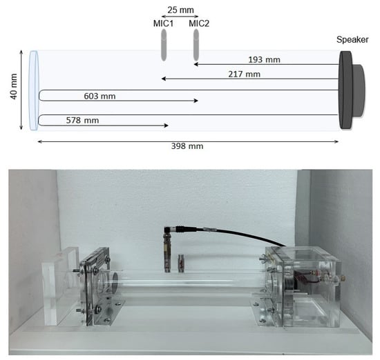
Figure 7.
Effective dimensions (top) and actual photograph (bottom) of the impedance tube used in the ISO 10534-2 measurements.
The working frequency range of the impedance tube is 300–4400 Hz: the lower frequency is limited by the accuracy of the signal processing equipment; the upper frequency depends only on the physical dimensions of the tube. The measurements were made with the so-called one microphone method: recording the tube response using one microphone in two different locations. This choice eliminates phase mismatch between microphones. According to ISO 10534-2 [26], the transfer function method was developed in MATLAB [30], using the tube impedance measurements scripts of the ITA-Toolbox [31].
The measurement chain consisted of a loudspeaker for the signal generation, a power supply, an audio device working with the audio stream input output (ASIO) drivers, a microphone and a battery power signal conditioner, as reported in Table 2.
Table 2.
Equipment used for the impedance tube measurements.
The output signal is an exponential sweep [32] converted to an analog signal by the digital-to-analog converter (DAC) of the audio device. The exponential sine sweep used for the experimental measurements was in the range of 250–5280 Hz, according to the working frequency range of the impedance tube (300–4400 Hz). The signal pressure coming from the microphone was converted to a digital audio object through an AD converter. All of the digital signal processing was developed in MATLAB with the help of the ITA-Toolbox impedance tube calculation scripts. The schematic is reported in Figure 8.
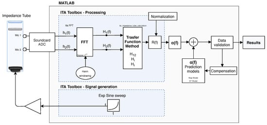
Figure 8.
Data flow: excitation signal generation, acquisition of the impulse responses and , processing, comparison with models, output of results.
The recorded audio file of length 2.97 s was sampled with a sample rate of 44,100 Hz at 24-bit depth, and a time data file of 131,072 samples was obtained.
3.3. Models Compensation
The experimental results for the MPP configurations showed some discrepancies between the measured data and both theoretical models decribed in Section 2. There were two important differences in common for each configuration:
- -
- A small frequency shift of the sound absorption peaks;
- -
- Absorption bandwidths larger than expected.
The first issue is connected to the samples’ mounting procedure (Figure 9).
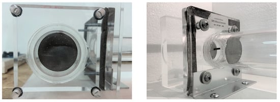
Figure 9.
Details of the sample MPP02 mounted inside the impedance tube.
All samples were rounded and had a diameter slightly smaller than the sample holder. This did not guarantee the samples to be firmly mounted inside the tube. In order to avoid the side gaps between the specimen and the tube and to respect the mechanical boundary conditions, small strips of adhesive tape were applied to clamp the edges as much as possible. This caused small vibrations of the samples and a part of the energy was dissipated through the adhesive strips, increasing the absorption bandwidth.
The absorption bandwidth is due to the variability of the geometrical parameters of the samples: mainly, the irregular shapes and sizes of the perforations are the reasons why the measured data bandwidths appear to be larger than the predicted ones [33,34]. In particular, the smaller the perforations were, the bigger were the discrepancies. The perforations’ perimeter was larger than expected and, consequently, a bigger absorption bandwidth occured. Instead of acting on the sample mounting procedure, a new compensating impedance has been added to the models, taking into consideration the discrepancies. Considering the electro-acoustic analogy of the single-layer MPPs, the following changes were applied:
- -
- , a resistance in series with the MPP impedance, associated to the dissipative losses due to the irregular perforations;
- -
- , a new inductance in parallel with the MPP surface impedance, associated with the displacement of air along the boundary of the sample and the sample vibration [35].
This is still valid for the double-layer configurations: furthermore, the mounting inaccuracy is emphasized by the doubling of the MPP layer. In a DL configuration, two different resistances in series with the MPP impedance and two inductances in parallel with the MPP impedances have been considered, one for every MPP layer. Thus, in order to consider the geometrical dimension issues of the steel samples and the main problem connected to the sample mounting procedure, some changes to the equivalent circuits were made, as shown in Figure 10.
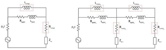
Figure 10.
Electro-acoustical equivalent circuit for SL-MPP and DL-MPP configurations: the inductance is in parallel with the MPP surface impedance , and the resistance is in series with .
The explicit equation of the surface impedance in the case of a DL-MPP configuration after compensation is the following:
In the present work, the values of and for the DL-MPP combinations were estimated by trial and error, trying to match the experimental data.
3.4. Specimen Properties
Three different SL configurations were measured, one for every type of sample (MPP01, MPP02, MPP03). A different value of the air cavity thickness was chosen for every MPP sample, in order to obtain a good sound absorption peak around 1000 Hz. The same was done for four different DL configurations, composed of the type of samples mentioned above. Two layers of MPP provide two different resonance peaks: the choice was to try to find DL configurations with an absorption peak at 1000 Hz and a second peak in a lower frequency range. The three samples had the effective geometrical parameters reported in Table 3.
Table 3.
Expected (exp.) and effective (eff.) geometrical parameters of the three MPP specimens.
The comparison between the equivalent fluid model and the experimental measurements is reported in terms of sound absorption coefficient and normalized surface impedance in Figure 11 for three SL configurations.
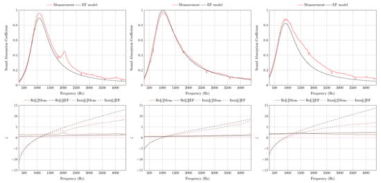
Figure 11.
Sound absorption coefficient and normalized surface impedance of single-layer MPPs: MPP01 with an air cavity of mm, MPP02 with an air cavity of mm and MPP03 with an air cavity of mm.
The three samples were used in four different combinations of DL configurations with air cavities reported in Table 4, and a comparison was made between the EF model and the experimental measurements in terms of sound absorption coefficient and normalized surface impedance in Figure 12. In contrast to the SL comparisons, the DL experimental measurements showed bigger discrepancies from the model: this is due to the mounting procedure inaccuracies and the irregular perforations of two different samples, both doubled. The model compensation is not enough to completely compensate for the non-idealities, mainly in terms of normalized surface impedance.
Table 4.
Specific normalised impedances corresponding to the four double-layer configurations. Octave band data were fitted based on the outcomes of the compensation model described in the text.
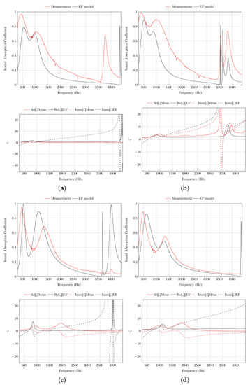
Figure 12.
Sound absorption coefficient and normalized surface impedance for four DL configurations. (a) Configuration A. (b) Configuration B. (c) Configuration C. (d) Configuration D.
4. Finite-Difference Time-Domain Simulations
In room acoustics, multiple simulation methods aim to directly solve the wave equation in homogeneous form:
where is the 3D Laplacian operator, is the speed of sound at °C and RH , and is the pressure (deviation from ambient). The finite-difference time-domain (FDTD) method is among the oldest numerical methods to solve time-dependent partial differential equations (PDEs), like the wave equation [36]. In FDTD methods, space and time continuous domains are typically discretized with regular Cartesian grids and updating recursions occur in the nodal points to calculate the acoustic properties such as the pressure or the particle velocity potential [37]. The solution of the wave equation, with , is approximated by a grid function at spatiotemporal points , , and , with l, m, n and p representing integer numbers, h the grid spacing, and k the time step [38,39]. A large variety of explicit FDTD methods follows the same general scheme:
where is the dimensionless quantity defined as the Courant number and a and b are the specific coefficients of a general family of compact explicit schemes [40]. The operators and act on as follows:
and similarly for and . The value of the Courant number is closely correlated to the stability condition of the system, which is guaranteed avoiding the exponential growth of the numerical solution (see, e.g., [41]). In the simple case of the seven-point scheme (a = b = 0), the stability condition is expressed as:
which is the so-called Courant–Friedrichs–Lewy (CLF) condition [36].
However, in this paper the cubic close-packed (CCP) scheme (see Figure 13), with , and = 1, is employed for its favorable numerical dispersion properties [41]. The consequent maximal time step, for a certain grid spacing, is k < h/c. As is the case for any 3D FDTD scheme, the computational cost is proportional to , which can quickly lead to large simulation grids. Then, such grid-based simulations are natural candidates for parallel acceleration on graphics processing units (GPUs) [42].
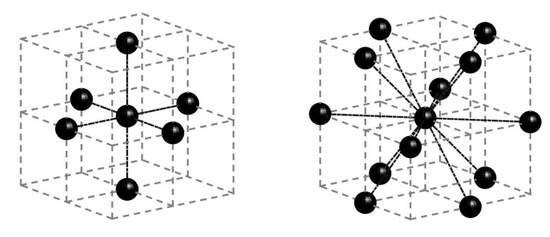
Figure 13.
Two possible stencils: standard 7-point (left) and cubic close-packed (CCP) 13-point (right). Image credit: see reference [28].
5. Application in a Case Study: Use of MPPs as a Ceiling Acoustic Treatment
A wide employment of sustainable materials such the multi-layer MPPs analyzed in this study is expected to occur in several typologies of enclosed environments [35,43], replacing or integrating the common sound absorbing treatments. MPP absorbers are theoretically expected to return the same acoustic behavior regardless of their constitutive material. Therefore, concerning sustainability aspects, they can be made of any green material, reducing the environmental footprint of the whole process. The acoustic simulation of a wide application in a 3D virtual enclosure is a useful tool in a preliminary step in the assessment of their performance [44,45,46].
With this purpose, the acoustic condition of a large university lecture hall has been simulated with a ceiling-mounted system of double-layer MPPs. Such a kind of large rooms shows the highest values of reverberation time at 500 and 1000 Hz (see Figure 4 in [27]), the same frequency range occupied by the human voice [47]. As too high values of reverberation time deteriorate speech intelligibility, a material whose sound absorbing properties are mostly centered in such a frequency range may return useful outcomes in acoustic treatments of existing university halls. Otherwise, an acoustic treatment with porous or fiber materials would provide the most significant absorbing contribution at higher frequencies [48], sometimes entailing too dry conditions at 2000 Hz and 4000 Hz.
The room chosen as a case study is a historical lecture hall in the University of Bologna (see Figure 14). A previous campaign of acoustic measurements [27,49] in the hall allowed to collect the main room criteria [50] and intelligibility indexes [47]. The setting of sound source and receiver locations chosen for the measurements campaign is also provided in Figure 14.
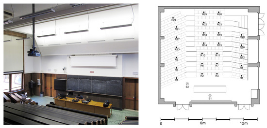
Figure 14.
Interior view (left) and 2D plan (right) of the lecture hall under study. Sound sources (S1, S2) and the spatial grid of microphone receivers (R1, R2, ..., RN) used in the measurements campaign are reported.
The 3D virtual model of the hall-about 900 m was built with Sketchup [51] according to consolidated approximation guidelines (see Figure 15), i.e., with a certain degree of geometrical approximation and with a proper division in macro-layers depending on the materials [52,53]. The 3D model was modeled using a small group of different materials (see Table 5) to reduce the uncertainties underlying the assignment of material properties to each surface. With regard to the absorption area distribution, it should be noted that, generally, the seats are the most sound absorbing objects in a lecture hall in unoccupied state [23,44,45,46]. The remaining layers of the model (walls, floor, ceiling) are made up of rather hard and reflective surfaces, and thus they show low values in the whole frequency range. It should also be highlighted that the random incidence absorption coefficients at low frequencies of wooden parts are due to the air cavity behind them (see dataset in Table 5).
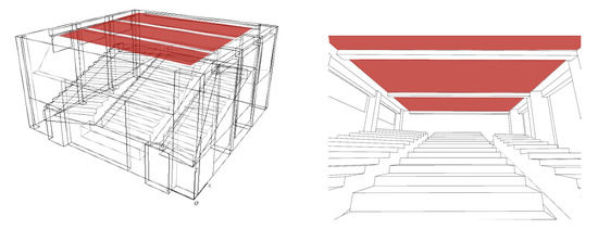
Figure 15.
Exterior (left) and interior (right) view of the acoustic treatment virtually introduced into the CAD model. The ceiling-mounted MPPs are highlighted in red.
Table 5.
Calibration setup (without MPP): random incidence absorption coefficients used in geometrical acoustics (GA) simulations and considered in the backward optimization process to obtain the acoustic admittances for the finite-difference time-domain (FDTD) simulation. The macro-layers used in the present work divide the materials into: hard/reflective surfaces (plaster floor), elements absorbing slightly at low frequencies (wood, windows) and the most sound absorbing area (seats).
The state-of-the-art procedure to simulate the sound field of a large lecture hall would imply the use of geometrical acoustics (GA) techniques [46,54]. Nevertheless, MPPs are not suitable to be characterized by the energy-based parameters, i.e., the absorption coefficients, usually involved in GA practice. Therefore, the need arose to simulate the acoustic behavior by using a wave-based algorithm, such as a FDTD model, that, additionally, assures the correct computation of the diffraction effects due to the objects’ edges [55].
With this purpose, in the 3D virtual model the edges of the blocks containing the seats and the long tables were modeled (see Figure 16b). The contour map shows the edge diffraction due to the seats, which are typically the only irregular element in a lecture hall contributing to the sound field diffusion. Figure 16 also shows a qualitative comparison with the standard GA simulation that involves a simpler modeling of the seats’ blocks and a scattering coefficient (see Figure 16a).
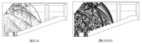
Figure 16.
Qualitative visualization of sound wave propagation within the lecture hall by means of GA (a) and FDTD (b) simulations throughout the longitudinal section. The sound source is located at the teacher’s position (S1 in Figure 14).
The DL-MPP corresponding to Configuration A in Table 4 was introduced in the model replacing most of the part of the existing false ceiling, as can be seen in Figure 15. Typically, the acoustic impedances needed as boundary conditions for an FDTD numerical simulation derive from the large amount of random incidence absorption coefficient datasets available through optimization processes [56]. Indeed, uncertainties inherent in energy parameters (absorption coefficients)—also due to ISO 354 limits [57]—are propagated in the conversion to non-unique corresponding complex acoustic impedances [58]. In this case, it has been possible to avoid some of those typical uncertainties in the workflow by directly starting with complex acoustic impedances values as input boundary conditions (see Figure 17) [59,60].
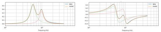
Figure 17.
Real (left) and imaginary (right) parts of complex specific admittances from data for MPP material (solid line) along with fitted filter model (dashed line) used in the FDTD simulation. Dotted lines show underlying resonances in the filter approximation.
Concerning the locally reactive absorption properties of the MPPs, the outcomes of the compensation model described in Section 3.3 were used to fit complex impedances to a boundary impedance model comprising a parallel network of second-order series RLC circuits [61]. The fitting procedure optimized non-negative circuit parameters (resistances, inductances and capacitances) in order to minimize the Euclidean norm of the error between the complex admittance of the circuit network and that of the data. A similar process was carried for known absorption coefficients of the remaining materials, following [62]. The complex admittance data and the model approximation to be used in the FDTD simulation are shown in Figure 17. As can be seen in the figure, the filter model described in [61,62] and used in the FDTD simulation faithfully reproduced the complex admittance of the MPP material.
The FDTD method chosen simulated up to 8000 Hz with 6.75 points per wavelength (Cartesian grid spacing mm and time step μs), which required approximately 2 h per sound source using four Nvidia Titan X (Maxwell) GPUs. It should be noticed that even though the FDTD model chosen in this work can switch to a ray-tracing algorithm over a certain frequency [63], in this case it was possible to run a full wave-based simulation thanks to the moderate complexity of the geometry and the availability of high computational power.
Before introducing the double-layer MPP into the virtual model of the lecture hall, the calibration process was carried out based on the main room criteria acquired from the acoustic measurements. The 3D model was tuned in terms of reverberation time () considering the sound source in location S1 and averaging the values over all the receiver points shown in Figure 14. Table 6 reports the trend in frequency of the measured values, the equivalent values derived from the calibrated FDTD model (“without MPP”) and the variations due to the introduction of MPPs (“with MPP”). During the tuning of the 3D model, the tolerance range for the discrepancies between measured and simulated values was kept equal to twice the common JND [50], considering 10% of the measured values according to recent remarks [64]. Table 6 also provides the mean values derived from the corresponding GA simulations to keep the comparison with the standard simulation procedure. Certainly in the GA model all of the temporal delays and acoustic behaviors due to the peculiarity of MPPs are approximated by energy parameters (absorption coefficients). With regard to the results in terms of reverberation time, the main contribution of the acoustic treatment is relevant at 500–1000 Hz, as expected, and still significant at 250 and 2000 Hz, due to the broadband performance obtained with DL configurations. The effects of treating a lecture hall with such a material instead of a common porous material are positive not only because they cover the frequency range occupied by the human voice, but also because they compensate for the typical excessive reverberation that undermines the verbal communication in historical rooms.
Table 6.
Trend in frequency of mean values corresponding to the results of the measurements (“Meas”), the equivalent values derived from the calibrated FDTD model (“without MPP”) and the variations due to the introduction of MPPs (“with MPP”). The mean values derived from the corresponding GA simulations are provided as a term of comparison.
Concerning the room criteria related to intelligibility, it is quite intuitive that in an optimal condition for the verbal communication their values should be as uniform as possible throughout the space. Therefore, the spatial behavior of sound clarity () [50] is provided versus the distance between the source and the receiver (see Figure 18). The same five conditions already seen in Table 6 are reported in the graph: the measured values, the calibration outcomes and the effects of the acoustic treatment according to FDTD and GA results. On average, it is possible to quantify an increase of values at mid frequencies higher than 4 dB, corresponding to four times the JND of the sound clarity. The acoustic treatment allowed to significantly increase the early-to-late ratio ( 2 dB) from a poor acoustic condition ( dB). Figure 18 also shows a good match among all the slopes of the linear regressions involved. This is probably due to the fact that the calibration was achieved by using an energy parameter, the reverberation time, that is derived from the energy decay curve as the sound clarity.
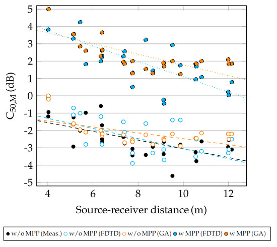
Figure 18.
Trend of sound clarity () as a function of the sound source-receiver distance (values and linear regressions). “M” indicates that the values have been averaged over 500 and 1000 Hz. Results of the measurements (“Meas”), the equivalent values derived from the calibrated FDTD model (“w/o MPP”) and the variations due to the introduction of MPPs (“w MPP”) are provided by using both FDTD and GA techniques.
Finally, an overview is provided about other recent works that handle the micro-perforated panels with wave-base simulation methods. Table 7 helps to place the present work in a framework of similar research studies to highlight similarities and methodological differences. Concerning the boundary conditions, it should be highlighted that only in reference [65] an extended reaction model for SL-MPP absorbers was used, including the incident angle dependence of surface impedance. In references [66,67] and in the present work the local reaction is assumed. To the best of the authors’ knowledge, at the time of writing there are several issues in handling extended reaction in FDTD and concurrently keeping the stability of the system. Indeed, in future developments further efforts will be made to improve the locally reactive simplified model used in the present work with the angle-dependent model.
Table 7.
Framework of recent works focused on wave-based simulations of micro-perforated panels. The frequency range managed by the authors, the calculation method, the typology of boundary condition employed and the output parameters obtained are reported.
6. Conclusions and Outlook
Sound absorbers based on MPPs could be an attractive alternative to the conventional porous and fibrous absorbers when following requirements such as durability, recyclability, cleanliness and environmental sustainability. Since MPP absorbers are theoretically expected to return the same acoustic behavior regardless of their constitutive material, in principle they can be made of any green material, provided that it is hard enough to support micro-perforation. In particular, stainless steel guarantees a long service life, being an unalterable material when applied indoors, and a good hygiene, being resistant to mold and fungi. A possible continuation of this research could be a detailed LCA analysis of a selection of materials usable to make MPP. The present work aims to outline a method for the design and the numerical validation of specific sound absorbers where both active and reactive acoustical properties have to be considered. Thanks to a full-spectrum FDTD simulation method the effects of this material on the intelligibility criteria were explored. First, three custom MPP specimens were designed and manufactured using a 3D additive metal printing process. The analytical predictive models of MPP in single- and double-layer configurations were validated through experimental measurements with the impedance tube obtaining the acoustical properties in terms of sound absorption coefficients and normalized surface impedances. Then, wider surfaces of double-layer MPPs were simulated in a calibrated 3D room corresponding to a real lecture hall. Results showed that MPPs mainly operate in the central octave band of 500 and 1000 Hz with a further useful contribution at 250 and 2000 Hz. Since this frequency range is the one most affecting speech intelligibility and at the same time the most undermined in historical lecture halls, MPPs seem to be a high-performance solution in cases similar to the present one. The university lecture hall taken as a case study is intended to show the positive effect of MPPs as acoustic treatment to the enhancement of speech intelligibility. In terms of time-dependence, the finite-difference time-domain model allowed us to better analyze both the reactive effects of the treatment and the scattering effects of the lecture hall’s geometry. Finally, for all these reasons the results of the present work should be indicate a robust method to experimentally measure and test the performance of specific materials, especially considering that the demand for high-performance and sustainable materials, such as the micro-perforated panels, is expected to increasingly grow in the sector of sound absorbing treatments.
Author Contributions
Conceptualization: M.G., D.D.; data curation: M.C.; formal analysis: D.D., M.G.; funding acquisition, M.G.; investigation, M.C. and L.B.; methodology, M.G., D.D.; project administration, M.G.; resources, L.B. and M.G.; MATLAB software: M.C. and M.G.; FDTD simulation, B.H. and G.F.; supervision, M.G., and D.D.; validation, M.C., D.D.; visualization, M.C. and G.F.; writing—original draft preparation, M.C. and D.D.; writing—review and editing, D.D., G.F., B.H. and M.G. All authors have read and agreed to the published version of the manuscript.
Funding
This research was funded by the Ministero dell’Istruzione dell’Università della Ricerca (Italy), in the framework of the project PRIN 2017, grant number 2017T8SBH9: “Theoretical modeling and experimental characterization of sustainable porous materials and acoustic metamaterials for noise control”.
Acknowledgments
The authors would like to thank Costantino Marmo, Donatella Alvisi and Nadia Perri, who kindly allowed us to carry out the acoustic measurements in the lecture hall taken as a case study.
Conflicts of Interest
The authors declare no conflict of interest.
Sample Availability
Samples of 3D MPPs are available from the authors.
References
- Pan, L.; Martellotta, F. A Parametric Study of the Acoustic Performance of Resonant Absorbers Made of Micro-perforated Membranes and Perforated Panels. Appl. Sci. 2020, 10, 1581. [Google Scholar] [CrossRef]
- Asdrubali, F.; Pispola, G. Properties of transparent sound-absorbing panels for use in noise barriers. J. Acoust. Soc. Am. 2007, 121, 214–221. [Google Scholar] [CrossRef]
- Sakagami, K.; Okuzono, T. Space sound absorbers with next-generation materials: Additional sound absorption for post-pandemic challenges in indoor acoustic environments. UCL Open Environ. Prepr. 2020. [Google Scholar] [CrossRef]
- Johnson, D.L.; Koplik, J.; Dashen, R. Theory of dynamic permeability and tortuosity in fluid-saturated porous media. J. Fluid. Mech. 1987, 176, 379–402. [Google Scholar] [CrossRef]
- Allard, J.F.; Champoux, Y. New empirical equations for sound propagation in rigid frame fibrous materials. J. Acoust. Soc. Am. 1992, 91, 3346–3353. [Google Scholar] [CrossRef]
- Cucharero, J.; Hänninen, T.; Lokki, T. Angle-Dependent Absorption of Sound on Porous Materials. Acoustics 2020, 2, 753–765. [Google Scholar] [CrossRef]
- Maa, D. Theory and design of microperforated panel sound-absorbing constructions. Sci. Sin. 1975, 18, 55–71. [Google Scholar]
- Maa, D. Microperforated-panel wideband absorbers. Noise Control Eng. J. 1987, 29, 77–84. [Google Scholar] [CrossRef]
- Maa, D. Potential of microperforated panel absorber. J. Acoust. Soc. Am. 1998, 104, 2861–2866. [Google Scholar] [CrossRef]
- Tayong, R.; Leclaire, P. Holes Interaction Effects under high and medium Sound Intensities for Micro-perforated panels design. In Proceedings of the 10th Congress Francais d’Acoustique, Lyon, France, 12–16 April 2010. [Google Scholar]
- Melling, T.H. The acoustic impendance of perforates at medium and high sound pressure levels. J. Sound Vib. 1973, 29, 1–65. [Google Scholar] [CrossRef]
- Atalla, N.; Sgard, F. Modeling of perforated plates and screens using rigid frame porous models. J. Sound Vib. 2007, 303, 195–208. [Google Scholar] [CrossRef]
- Cobo, P.; Simon, F. Multiple-Layer Microperforated Panels as Sound Absorbers in Buildings: A Review. Buildings 2019, 9, 53. [Google Scholar] [CrossRef]
- Lee, D.H.; Kwon, Y.P. Estimation of the absorption performance of multiple-layer perforated panel systems by transfer matrix method. J. Sound Vib. 2004, 278, 847–860. [Google Scholar] [CrossRef]
- Sakagami, K.; Morimoto, M.; Koike, W. A numerical study of double-leaf microperforated panel absorbers. Appl. Acoust. 2019, 2006, 67–609. [Google Scholar] [CrossRef]
- Hoshi, K.; Hanyu, T.; Okuzono, T.; Sakagami, K.; Yairi, M.; Harada, S.; Takahashi, S.; Ueda, Y. Implementation experiment of a honeycomb-backed MPP sound absorber in a meeting room. Appl. Acoust. 2020, 157, 107000. [Google Scholar] [CrossRef]
- Tsay, Y.S.; Yeh, C.Y. A Machine Learning Based Prediction Model for the Sound Absorption Coefficient of Micro-Expanded Metal Mesh (MEMM). Appl. Sci. 2020, 10, 7612. [Google Scholar] [CrossRef]
- Arvidsson, E.; Nilsson, E.; Hagberg, D.B.; Karlsson, O.J. The Effect on Room Acoustical Parameters Using a Combination of Absorbers and Diffusers—An Experimental Study in a Classroom. Acoustics 2020, 2, 505–523. [Google Scholar] [CrossRef]
- Choi, Y. Evaluation of acoustical conditions for speech communication in active university classrooms. Appl. Acoust. 2020, 159, 107089. [Google Scholar] [CrossRef]
- D’Orazio, D.; De Salvio, D.; Anderlucci, L.; Garai, M. Measuring the speech level and the student activity in lecture halls: Visual-vs blind-segmentation methods. Appl. Acoust. 2020, 169, 107–448. [Google Scholar] [CrossRef]
- Brill, L.C.; Smith, K.; Wang, L.M. Building a sound future for students: Considering the acoustics of occupied active classrooms. Acoust. Today 2018, 14, 14–22. [Google Scholar]
- Hodgson, M.; Rempel, R.; Kennedy, S. Measurement and prediction of typical speech and background-noise levels in university classrooms during lectures. J. Acoust. Soc. Am. 1999, 105, 226–233. [Google Scholar] [CrossRef]
- Puglisi, G.E.; Bolognesi, F.; Shtrepi, L.; Warzybok, A.; Kollmeier, B.; Astolfi, A. Optimal classroom acoustic design with sound absorption and diffusion for the enhancement of speech intelligibility. J. Acoust. Soc. Am. 2017, 141, 3456–3457. [Google Scholar] [CrossRef]
- Visentin, C.; Prodi, N.; Cappelletti, F.; Torresin, S.; Gasparella, A. Using listening effort assessment in the acoustical design of rooms for speech. Build Environ. 2018, 136, 38–53. [Google Scholar] [CrossRef]
- Chung, J.Y.; Blaser, D.A. Transfer function method of measuring induct acoustic properties. I. Theory. J. Acoust. Soc. Am. 1980, 68, 907–913. [Google Scholar] [CrossRef]
- EN ISO 10534–2:2001. Acoustics-Determination of Sound Absorption Coefficient and Impedance in Impedance Tubes-Part.2: Transfer-Function Method; International Organization for Standardization: Geneva, Switzerland, 2001. [Google Scholar]
- Fratoni, G.; D’Orazio, D.; De Salvio, D.; Garai, M. Predicting speech intelligibility in university classrooms using geometrical acoustic simulations. In Proceedings of the 16th IBPSA, Rome, Italy, 2–4 September 2019. [Google Scholar]
- Hamilton, B.; Webb, C.J. Room acoustics modelling using GPU-accelerated finite difference and finite volume methods on a face-centered cubic grid. In Proceedings of the Digital Audio Effects (DAFx), Maynooth, Ireland, 2–6 September 2013; pp. 336–343. [Google Scholar]
- Ning, J.F.; Ren, S.W.; Zhao, G.P. Acoustic properties of micro-perforated panel absorber having arbitrary cross-sectional perforations. Appl. Acoust. 2016, 111, 135–142. [Google Scholar] [CrossRef]
- MATLAB, Version 9.6.0.1072779 (R2019a); The MathWorks Inc.: Natick, MA, USA, 2019.
- ITA-Toolbox, Open source MATLAB toolbox for acoustics developed by the Institute of Technical Acoustics of the RWTH Aachen University, Neustrasse 50, 52056, Aachen, Germany. In Proceedings of the DAGA 2017, Kiel, Germany, 6–9 March 2017.
- Corredor-Bedoya, A.C.; Acuña, B.; Serpa, A.L.; Masiero, B. Effect of the excitation signal type on the absorption coefficient measurement using the impedance tube. Appl. Acoust. 2020, 171, 107659. [Google Scholar] [CrossRef]
- Sakagami, K.; Kusaka, M.; Okuzono, T.; Nakanishi, S. The Effect of deviation due to the manufacturing accuracy in the parameters of an MPP on its acoustic properties: Trial production of MPPs of different hole shapes using 3D printing. Acoustics 2020, 2, 605–606. [Google Scholar] [CrossRef]
- Randeberg, R.T. Perforated Panel Absorbers with Viscous Energy Dissipation Enhanced by Orifice Design. Ph.D. Dissertation, Department of Telecommunication, Norwegian University of Science and Technology, Trondheim, Norway, June 2000. [Google Scholar]
- Sakagami, K.; Morimoto, M.; Yairi, M. A note on the effect of vibration of a microperforated panel on its sound absorption characteristics. Acoust. Sci. Technol. 2005, 26, 204–207. [Google Scholar] [CrossRef]
- Courant, R.; Friedrichs, K.; Lewy, H. Über die partiellen Differenzengleichungen der mathematischen Physik. Math. Annal. 1928, 100, 32–74. [Google Scholar] [CrossRef]
- Botteldooren, D. Finite-difference time-domain simulation of low-frequency room acoustic problems. J. Acoust. Soc. Am. 1995, 98, 3302–3308. [Google Scholar] [CrossRef]
- Bilbao, S.D. Numerical Sound Synthesis; John Wiley & Sons: Hoboken, NJ, USA, 2009. [Google Scholar]
- Savioja, L. Real-time 3D finite-difference time-domain simulation of low-and mid-frequency room acoustics. In Proceedings of the 13th International Conference on Digital Audio Effects, Maynooth, Ireland, 6–10 September 2010. [Google Scholar]
- Kowalczyk, K.; Van Walstijn, M. Room acoustics simulation using 3-D compact explicit FDTD schemes. IEEE Trans. Audio Speech Lang. Process. 2011, 19, 34–46. [Google Scholar] [CrossRef]
- Hamilton, B. Finite Difference and Finite Volume Methods for Wave-Based Modelling of Room Acoustics. Ph.D. Dissertation, University of Edinburgh, Edinburgh, UK, 2016. [Google Scholar]
- Micikevicius, P. 3D finite difference computation on GPUs using CUDA. In Proceedings of the 2nd Workshop on General Purpose Processing on Graphics Processing Units, Washington, DC, USA, 8 March 2009; pp. 79–84. [Google Scholar]
- Arenas, J.P.; Sakagami, K. Sustainable Acoustic Materials; MDPI: Basel, Switzerland, 2020; p. 6540. [Google Scholar]
- Bistafa, S.R.; Bradley, J.S. Predicting speech metrics in a simulated classroom with varied sound absorption. J. Acoust. Soc. Am. 2001, 109, 1474–1482. [Google Scholar] [CrossRef] [PubMed]
- Reich, R.; Bradley, J. Optimizing classroom acoustics using computer model studies. Can. Acoust. 1998, 26, 15–21. [Google Scholar]
- Bistafa, S.R.; Bradley, J.S. Predicting reverberation times in a simulated classroom. J. Acoust. Soc. Am. 2000, 108, 1721–1731. [Google Scholar] [CrossRef]
- IEC 60268-16. Sound System Equipment–Part 16: Objective Rating of Speech Intelligibility by Speech Transmission Index; IEC: Geneva, Switzerland, 2020. [Google Scholar]
- Garai, M.; Pompoli, F. A simple empirical model of polyester fibre materials for acoustical applications. Appl. Acoust. 2005, 66, 1383–1398. [Google Scholar] [CrossRef]
- Martellotta, F. Optimizing stepwise rotation of dodecahedron sound source to improve the accuracy of room acoustic measures. J. Acoust. Soc. Am. 2013, 134, 2037–2048. [Google Scholar] [CrossRef]
- ISO 3382-2. Acoustics-Measurement of Room Acoustic Parameters-Part 2: Reverberation Time in Ordinary Rooms; International Organization for Standardization: Geneva, Switzerland, 2008. [Google Scholar]
- SketchUp, Trimble Inc., Version Make, 935 Stewart Drive, Sunnyvale CA (USA) 94085. 2017.
- Vorländer, M. Auralization; Springer: Aachen, Germany, 2008. [Google Scholar]
- Postma, B.N.; Katz, B.F. Perceptive and objective evaluation of calibrated room acoustic simulation auralizations. J. Acoust. Soc. Am. 2016, 140, 4326–4337. [Google Scholar] [CrossRef]
- Choi, Y.J. Effects of periodic type diffusers on classroom acoustics. Appl. Acoust. 2013, 74, 694–707. [Google Scholar] [CrossRef]
- Okuzono, T.; Shadi, M.; Sakagami, K. Potential of Room Acoustic Solver with Plane-Wave Enriched Finite Element Method. Appl. Sci. 2020, 10, 1969. [Google Scholar] [CrossRef]
- Mondet, B.; Brunskog, J.; Jeong, C.H.; Rindel, J.H. From absorption to impedance: Enhancing boundary conditions in room acoustic simulations. Appl. Acoust. 2020, 157, 106884. [Google Scholar] [CrossRef]
- Vercammen, M. On the Revision of ISO 354, Measurement of the Sound Absorption in the Reverberation Room; ISO/WD: Geneva, Switzerland, 2018. [Google Scholar]
- Jeong, C.H. Converting Sabine absorption coefficients to random incidence absorption coefficients. J. Acoust. Soc. Am. 2013, 133, 3951–3962. [Google Scholar] [CrossRef]
- Takumi, Y.; Okuzono, T.; Sakagami, K. Locally implicit time-domain finite element method for sound field analysis including permeable membrane sound absorbers. Acoust. Sci. Technol. 2020, 41, 689–692. [Google Scholar]
- Cheng, Y.; Cheng, L.; Pan, J. Absorption of oblique incidence sound by a finite micro-perforated panel absorber. J. Acoust. Soc. Am. 2013, 133, 201–209. [Google Scholar]
- Bilbao, S.; Hamilton, B.; Botts, J.; Savioja, L. Finite volume time domain room acoustics simulation under general impedance boundary conditions. In IEEE-ACM Transactions on Audio, Speech, and Language Processing; IEEE: Piscataway, NJ, USA, 2016; Volume 24, pp. 161–173. [Google Scholar]
- Hamilton, B.; Webb, C.J.; Fletcher, N.D.; Bilbao, S. Finite difference room acoustics simulation with general impedance boundaries and viscothermal losses in air: Parallel implementation on multiple GPUs. In Proceedings of the Int. Symp. Musical Room Acoust, La Plata, Argentina, 11–13 September 2016. [Google Scholar]
- D’Orazio, D.; Fratoni, G.; Rovigatti, A.; Hamilton, B. Numerical simulations of Italian opera houses using geometrical and wave-based acoustics methods. In Proceedings of the 23rd International Congress on Acoustics, Aachen, Germany, 9–13 September 2019. [Google Scholar]
- Vorländer, M. Computer simulations in room acoustics: Concepts and uncertainties. J. Acoust. Soc. Am. 2013, 133, 1203–1213. [Google Scholar] [CrossRef] [PubMed]
- Okuzono, T.; Sakagami, K. A frequency domain finite element solver for acoustic simulations of 3D rooms with microperforated panel absorbers. Appl. Acoust. 2018, 129, 1–12. [Google Scholar] [CrossRef]
- Okuzono, T.; Sakagami, K. A finite-element formulation for room acoustics simulation with microperforated panel sound absorbing structures: Verification with electro-acoustical equivalent circuit theory and wave theory. Appl. Acoust. 2015, 95, 20–26. [Google Scholar] [CrossRef][Green Version]
- Toyoda, M.; Eto, D. Prediction of microperforated panel absorbers using the finite-difference time-domain method. Wave Motion 2019, 86, 110–124. [Google Scholar] [CrossRef]
- Liu, J.; Herrin, D.W. Enhancing micro-perforated panel attenuation by partitioning the adjoining cavity. Appl. Acoust. 2010, 71, 120–127. [Google Scholar] [CrossRef]
- Naderyan, V.; Raspet, R.; Hickey, C.J.; Mohammadi, M. Acoustic end corrections for micro-perforated plates. J. Acoust. Soc. Am. 2019, 146, EL399–EL404. [Google Scholar] [CrossRef]
Publisher’s Note: MDPI stays neutral with regard to jurisdictional claims in published maps and institutional affiliations. |
© 2021 by the authors. Licensee MDPI, Basel, Switzerland. This article is an open access article distributed under the terms and conditions of the Creative Commons Attribution (CC BY) license (http://creativecommons.org/licenses/by/4.0/).