Article

The Impact of Skinsuit Zigzag Tape Turbulators on Speed Skating Performance

Faculty of Aerospace Engineering, Delft University of Technology, 2629HS Delft, The Netherlands
*
Author to whom correspondence should be addressed.
Appl. Sci. 2021, 11(3), 988; https://doi.org/10.3390/app11030988
Submission received: 31 December 2020 / Revised: 19 January 2021 / Accepted: 20 January 2021 / Published: 22 January 2021
(This article belongs to the Special Issue Sports Fluid Mechanics)

Abstract

:
At the 1998 Nagano Winter Olympic Games, zigzag tape was introduced on the race suit lower legs and cap of speed skaters. Application of these zigzag devices on live skaters and cylinders in the wind tunnel showed large improvements in the aerodynamic drag. These wind-tunnel results were unfortunately not widely published, and the impact of the zigzag strips in a real skating environment was never established. This paper aims to show the background of the application of the zigzag tape and to establish the impact it may have had on speed-skating performance. From comparisons of 5000 m races just before, during and just after the Nagano Olympics and an analysis of historic world record data of the 1500 m men’s speed skating, the impact of the zigzag tape turbulators on average lap times on 1500 and 5000 m races is calculated to be about 0.5 s.

1. Introduction

During the past decades, research and innovations in the field of sport apparel and materials have helped to increase skating speed tremendously. The introduction and fine-tuning of the clap skate mechanism, the thickness and metal compound of blades and the application of water-additives to reduce ice-friction all had their impact on improved speed-skating performance [1]. Skating suits evolved from the knitted outfits used during the early 1970s to the present suits with distributed rough patches [2,3].
In the almost 25 years following the introduction of the one-piece skinsuit by the Austrian Franz Krienbühl, in 1974/75 until February 1998, the suits worn by elite speed skaters developed gradually, mostly aiming at a better fit and at improved cooling characteristics. While until 1998 the trend was to use increasingly smooth fabrics, at the 1998 Nagano Olympics, foam zigzag tape strips on the lower legs and the cap of the skating suit were introduced, aiming at significant aerodynamic drag reduction, Figure 1. The application of the zigzag tape to racing suits by the Dutch team followed earlier measurements by Eise Dobbinga, a Delft University of Technology (TU Delft) aerodynamics professor who experimentally investigated the impact of trip wires and seams on the aerodynamic drag of cylinders and a mannequin leg covered with a skinsuit fabric [4]. He found that the drag coefficient of such a mannequin leg could be reduced by 22% when the entire leg was equipped with a 0.8 mm thick trip wire on both sides of the leg front end. These results unfortunately lay dormant for over 10 years, until in 1997 and January 1998, wind-tunnel measurements at TU Delft were performed on live skaters and cylinders, this time using zigzag tape as a turbulator. Zigzag tape proved to be an efficient means to trip the laminar boundary layer on a sailplane wing, thus avoiding drag rise due to laminar separation at low Reynolds numbers. This flow phenomenon is typically also present around the body of speed skaters with smooth skinsuits. Total drag area reductions on static male skaters with zigzag-tape strips on lower legs and cap were found up to 9%. Although some results were presented in low-circulation media [5,6,7,8], unfortunately little of this work on the impact of zigzag tape, specifically on speed-skating performance, has been widely published.
The Dutch team was quite successful in Nagano; they gathered more gold medals than ever before. Although the wind-tunnel tests were very promising, the contribution of the zigzag strips to reduce the aerodynamic drag in the actual races remained unclear. The aim of this paper is to present results of wind-tunnel measurements showing the effects of the strips and, in addition, to quantify the impact on speed skating performance the zigzag strips may have had in a real skating environment.

2. The Flow over the Lower Legs

The flow over bluff objects with rounded edges is typified by the Reynolds number. It describes the ratio of the inertia forces (in terms of flow speed V, characteristic length L and density ρ) over the viscous forces (in terms of the dynamic viscosity µ) in the flow:
Re = ρ . V . L μ
For cylinders and spheres, the characteristic length is the diameter, D. The Re-number is closely related to the laminar-to-turbulent transition location of the boundary layer flow along the surface of an object and the resulting drag. Transition is a delicate process, which is not only influenced by the shape of the object and its orientation towards the incoming flow, but also by its surface roughness and by disturbances in the flow, such as free-stream turbulence. For bluff bodies, such as cylinders and spheres, there is a significant drag reduction (the “drag crisis”) at a certain Re-number, called the critical Reynolds number, due to the boundary layer flow becoming turbulent before separation, which leads to a smaller drag and a higher wake static pressure, compared to a situation with laminar separation. For lower (sub-critical) Reynolds numbers, the flow is mostly laminar. Although a laminar boundary layer has a lower friction drag than a turbulent layer, it has the disadvantage of losing its momentum close to the wall of the object relatively fast, resulting in separation of the flow from the object, even prior to reaching the thickest point. This leads to a large wake with a low pressure, which, combined with the stagnation pressure at the leading edge of the object, results in a high pressure drag.
It is long known that this pressure drag of circular cylinders in the sub-critical Reynolds number regime can be significantly reduced by tripping the laminar boundary layer, forcing it to become turbulent [9,10], thus adding momentum to the lower part of the boundary layer, helping it to flow against the strong adverse pressure gradient at the back of the cylinder, which postpones the separation of the boundary layer, increases the static pressure in the wake and reduces the size of the wake.
The measurements of the effect of trip wires on the drag of a model leg presented in Reference [4] showed strong resemblance with the flow around a two-dimensional cylinder. Although the cross-section varies and the drag values are different, the flow mechanisms are quite comparable.
The impact of zigzag tape on the flow around a leg is presented in Figure 2, using the fluorescent-oil-flow visualization technique. The pictures were taken in the Delft University 1.25 × 1.80 m, of low-speed low-turbulence wind tunnel (LTT), using the same mannequin leg as in Reference [4]. The flow over the leg was visualized with a UV lamp. In the left picture, the light yellow band shows a laminar separation bubble, following a laminar region and the subsequent turbulent separation with reversed flow. Darker areas point at a higher surface shear stress, which transports the oil in flow direction. In the right picture, clearly the small tape-induced vortices can be seen, which make the flow turbulent and move the separation location more backwards, reducing the pressure drag.

3. Measurements

3.1. Cylinder Measurements

To determine a frame of reference for a suitable location and thickness of the zigzag tape on the legs in relation to the Reynolds number, a number of wind-tunnel tests were dedicated to the flow over a cylinder.
In a first series of tests, a polished plastic cylinder with circular cross-section was used with a diameter of 11 cm and a span of 60 cm, later on followed by a second series on a 90 cm span cylinder with the same diameter. The measurements were performed in the TU Delft LTT. The turbulence intensity in the tunnel ranges from 0.02% to 0.07% in a speed range from 10 to 75 m/s. Figure 3 shows the front view of the setup with the 90 cm span cylinder. The tests on the smaller span were performed in a similar manner, with a higher table. The cylinder was attached to a circular disc flush with the tunnel wall, and rotated with the mechanical 6-component external balance system. The forces were recorded with a frequency of 5Hz and averaged over 10 s.
In view of the strong dynamics in the flow, the sampling time of 5 Hz might seem very low; however, due to the inertia of the balances (rotating spindles with running weights), strong fluctuations will not be followed, which already averages out large and fast variations effectively. The gap between the cylinder lower end and the table was kept within 0.5 mm. All measurements were corrected for wind-tunnel blockage with the method of Maskell described in Reference [11], using a blockage factor, ε = 0.96. The drag coefficient was calculated from the following:
C D = D qA
where D is the measured drag force, q is the test section dynamic pressure following from a dedicated calibration and A is the model frontal area. Figure 4 presents the azimuth dependency of the drag coefficients for 0.93 mm thick zigzag tape. It shows that placing the tape too close to the leading edge at low Reynolds numbers does not lead to sufficient destabilization of the laminar boundary layer to generate turbulent flow at lower wind speeds. Tape with this thickness requires a higher Reynolds number to effectively trigger transition. When placed too far downstream, the laminar boundary layer is already too thick for the tape to add sufficient momentum to the lower part of the boundary layer in order to effectively suppress early separation.
Figure 5 shows the effect of tape thickness at an azimuth angle of 30° on the same cylinder. For drag reduction at a lower Reynolds number, a higher tape thickness is required, as expected. Depending on the Reynolds number range the zigzag tape should do its work in, the tape location and thickness can be estimated.

3.2. Mannequin Leg Measurements: The Effect of Angle of Attack

As the zigzag tape is at fixed positions on the contour, the mannequin leg was also used to study the sensitivity to angle-of-attack changes. Figure 6 shows a typical example of such a measurement. It demonstrates the effect of zigzag tape on the model drag coefficient in the angle of attack range between −15° and 15°, measured with the tunnel 6-component balance system. The reference frontal area is 0.07 m2; the Reynolds number is based on an average equivalent diameter of the lower leg (circumference divided by π) of 8.6 cm. The tape was placed with the trailing edge at a 55-degree equivalent azimuth angle. Despite the fact that the tape thickness and location might not be optimal at this Reynolds number, for negative angles, the drag reduction due to the zigzag tape is about 10%, while, at a positive angle of 15°, the reduction decreases, but still has an acceptable value of 4%. Positive angles are measured clockwise. In this case, the lower-leg frontal area is 52% of the total, giving a lower-leg maximum drag reduction comparable with the total leg-drag reduction of Dobbinga of 22%

3.3. Static Skater Measurements

Measurements on live skaters were performed in the 2.2 m diameter open jet facility of TU Delft’s Wind Energy Institute. The purpose of the tests was twofold: to study the posture of a number of Dutch elite speed skaters and to determine the effectiveness of zigzag tape when used by real skaters. Figure 7 shows a schematic of the test setup, using a simple one-component strain gauge balance system to measure the drag force. The skaters were either placed on two small wooden blocks or used their own skates to stand on.

3.3.1. Method

As the drag heavily depends on frontal area, the skater was asked to take his skating position five times in a row, departing from an upright position. The variation in measured drag is strongly dependent on the skater’s ability to resume and maintain this skating position. The skaters were helped in this respect by ensuring that the distance between the ground plate of the balance and a marker on their rear was constant at the beginning of each run, to secure a constant knee angle. The drag force was recorded during 4 s, with a frequency of 250 Hz, and averaged. Zero-wind balance readings with the skater in skating position were subtracted from the wind-on values. The measurements were also corrected for temperature variation; for the effects of nozzle and solid blockage on the dynamic pressure, which is calculated to be about 2%; and for the additional drag of the support (small blocks and/or plate) the skater was standing on.

3.3.2. Results

Figure 8 presents the measured drag area of a male long-distance skater for three configurations: the impact of 0.5 mm thick Teflon zigzag tape (also depicted in Figure 5) on the lower legs and of 0.75 mm thick zigzag tape on the cap. The averages over the five runs are tabulated in Table 1.

Zigzag Tape on the Lower the Legs

Looking at the standard deviation, σ, shown in Table 1, we see that the followed procedure gives reasonably steady results for the conditions with no tape on the cap. The race suit used for the tests was made of Coolmax, a polyester fabric, following the trend of those days, which was to use increasingly smooth breathable fabrics. The values in Table 1 indicate an average reduction of the total drag of the skater due to the zigzag tape on the lower legs of 8.6%. With a frontal area of the lower legs of about 20% of the total for this particular skater, this means a drag reduction of the lower legs of roughly 40%, which is 20% per leg. It must be noted that the turbulence intensity of the open jet wind tunnel was in the order of 0.8%. Increased small-scale turbulence promotes boundary layer transition, which, in this case, might have led to a reduction in drag for the smooth suit already, compared to a situation with relatively low turbulence, such as the case of an isolated skater on an indoor skating rink. Furthermore, the tape was at an azimuth position of 55 degrees, which, in combination with the 0.5 mm thick tape (on the thin side according to Figure 5), may not have led to a maximum drag reduction.

Zigzag Tape on the Cap

Despite the right starting position, there is a large variation in the drag area of the configuration with zigzag tape on the cap only. Without any other known explanation (during these very first tests, changes in posture were not constantly recorded by a camera), this might be due to the fact that the drag of the head is actually reduced, which may feel (and perhaps also sound) unfamiliar to the skater and may have led to variation of the position of the head or even the trunk during the runs. The impact of the tape on the cap of this particular skater is rather inconclusive, given the large spread in the data. Based on the averages, the application of the zigzag tape on the cap led to a total drag reduction of 4.3%. Tests on a female skater with zigzag tape on the cap, in the same test campaign, gave a reduction of up to 2.8% on overall drag (σ = 0.9%). Later measurements have shown that zigzag tape on the cap indeed can have a significant effect on the total drag, as it results in attached flow over a larger part of the head, which may have a strong positive influence on the flow over the back. Wind-tunnel tests in 2004 (in a different facility) revealed that the drag of a male skater wearing the Nike 2002 Olympic suit could be reduced with a little over 3% (σ = 0.6%) by applying zigzag tape with the right thickness and position on the cap. At present, it seems that skinsuit manufacturers underestimate the possible contribution of improving the flow over the head to lower drag.

4. The Reynolds Number of the Flow around a Speed Skater’s Leg

An estimation of the Reynolds number range of a male speed skater’s lower legs at the time of the introduction of the strips was based on the December 1997 world-record average speeds, at 1500 and 5000 m. The expected variation in Reynolds number due to the movement of the legs was estimated to be about 15% for the calf and 20% for the ankle. In a later stage, this variation was addressed more accurately. Looking at the stroke frequency at distances of 1500 m and longer, the forward deflection of the legs and the time of the stroke cycle, De Koning [12] came to an additional average over speed during the cycle relative to the body for the calf of about 2.6 m/s and for the ankle of about 4 m/s. Table 2 lists the parameters used in the calculation of the Reynolds number. The density (ρ) and dynamic viscosity (μ) are 1.234 kg/m3 and 1.802 × 10⁻⁵ Pa.s, respectively, based on dry air at a temperature of 13 degrees Celsius and a standard sea level ambient pressure of 1013.25 hPa. The equivalent diameter (Deq) was based on the calf and ankle average circumferences of five mail elite skaters competing on the longer distances.
Table 2 shows that the variation in Reynolds number is quite substantial: about 20% for the calf and 30% for the ankle. This is important information, since the aerodynamic behavior of the leg should be tuned in just the right Reynolds number range. In fact, the Re range is even a little bit wider, given the fact that we depart from the average speed, while, especially during a 1500 m race, lap speed drops towards the end. For the calf of the leg with a Reynolds number range of approximately 0.87× 10⁵ to 1.4× 10⁵ for 1500 and 5000 m races, Figure 4 shows us that, for a cylinder, an azimuth position between 40° and 45° would give a sufficiently low CD. For the ankle with a range from 0.46× 10⁵ to 0.8× 10⁵, an angle not lower than 45° is required. For the male skaters in Nagano, this was translated into an instruction to take the local circumference of the lower leg, take one ninth (calf) or one eighth (ankle) of this and locate the front of the zigzag strips at this distance, to the left and the right from the leg leading edge. In terms of azimuth angle on a cylinder with a diameter equal to the equivalent diameter (circumference divided by π) of the leg, this is approximately 40° and 45°, respectively. For the female skaters, this was one-eighth for both locations, since their legs have a lower Reynolds number. In this configuration, the drag of the cylinder in Figure 4 is reduced with 50%, compared to an average 20% reduction for a male skater’s lower leg with a thinner tape, as presented earlier.

5. The Impact of the Zigzag Strips on Skating Performance in a Real Skating Environment

The wind-tunnel tests discussed in the previous sections have shown that, in well-controlled static conditions, the zigzag tape strips may lead to a significant decrease in the aerodynamic drag. In actual races, this reduction will have been much lower since in the curves, which take about half of the track length, the position of the legs will deviate from the wind-tunnel configuration. The right leg will alternately be stretched, raising the drag area, or partly cover the lower left leg, while undergoing an angle of attack change towards the incoming wind for part of the curve. Furthermore, one arm swinging freely in the flow (like is always done in the curves) also raises the drag area. Taking all this into account, the total gain of using zigzag strips on the lower legs and cap during races was estimated to be about 4% to 5% for the male skaters tested. Unfortunately, the period in which there existed a difference between skaters that actually wore the zigzag strips and those who did not is very limited. Already during the Nagano Games other teams recognized the potential benefit and also applied the strips (e.g., the Norwegian team). Hence, there is little material for a thorough statistical analysis. Nevertheless, in view of the large impact that turbulators have on the aerodynamics of skaters, whether it is zigzag tape or rough fabrics, differences must be retrievable from the results, albeit probably with less accuracy a statistical study with a large number of realizations might produce. In the following, an attempt is made to quantify the impact of the zigzag strips, by approaching the matter from three different angles.

5.1. Looking Closer at the 1998 Nagano Results

The first analysis is based on three consecutive 5000 m events in 3.5 months’ time, just before, at and just after the 1998 Nagano Olympic games in which Dutchman Gianni Romme came out as a winner. Since these were all world records, this enables us to compare his performance in the three races, assuming he constantly used his average optimum power. To investigate this in more detail, let us look at the three races, starting in Heerenveen, the Netherlands (Thialf venue), during a world cup meeting on 7 December 1997 (without drag reducing zigzag strips) and ending in Calgary, Canada (Olympic Oval), during the World Championships Single Distances on 27 March 1998, where all the top 10 skaters used the zigzag strips.
To determine how much power a skater puts in his propulsion, generally, a simple Equation (3) can be used:
P req = 1 2 ρ V 3 C D A + μ mgV
It combines the average power required to overcome the aerodynamic drag force of the skater, in which CD is the average drag coefficient, A is the frontal area and ρ is the local air density, and the average ice friction force with µ, the ice friction coefficient; m, the mass of the skater; and g, the gravitational acceleration. For momentary velocities, eq. 3 is not suited, since a term covering the accelerations is omitted.
To calculate Romme’s average required power, a value of 0.275 for the drag area CDA was used following from the equations suggested by van Ingen Schenau [13], with a correction on the basis of the open jet measurements reported above. The skater’s mass and length were taken to be 85 kg and 1.90 m [14].
References [1,15] give a variety of values for the ice-friction coefficient. Reference 1 mentions a value of present day friction coefficients in ice rinks as low as 0.0025. To account for developments in blade material and thickness and experience in ice preparation since 1997, the friction coefficient was set at 0.004. Table 3 presents the calculated required power for the two extremes in density: Heerenveen and Calgary, on the basis of the parameters mentioned above, so without accounting for drag reducing devices in Calgary. The barometric pressures were taken from historic weather data of stations near the venues [16] (Leeuwarden air base at 38 km distance, sea level, and Calgary International Airport at 18 km distance, altitude 1099 m) around the time of the day the races were held. With the local pressure and temperature given, the densities were calculated for the respective elevations (0 and 1034 m). As there is no public record of the temperatures in Thialf and the Olympic Oval, they were taken equal to the one measured during the Nagano race given in the official report published by the Nagano Winter Games organizing committee [17].
One would expect that, with a power available of 398 Watts in Heerenveen, the speed in Calgary due to the substantially lower air density would be much higher (13.335 m/s, according to Equation (1)). However, the average speed of 13.107 m/s requires an estimated power of only 379 Watts, with an unchanged drag area, the power for a configuration with an assumed decreased drag due to zigzag strips even being lower. The rink temperature and the ice friction coefficients may have differed from the assumptions, but by far not to the degree that it covers the missing power of 21 Watts. For a matching power, the rink temperature in Heerenveen should have been 29 °C, or the ice friction coefficient in Calgary should have been 42% higher compared to Thialf. Considering the fact that at both occasions a world record was skated, the circumstances will have been quite optimal for both well-known ice rinks.
This power dissimilitude at sea level and altitude was already addressed by van Ingen Schenau in the early nineties of the last century [18]. More recently, Van Erck et al. [19] showed that a reduction in gross efficiency of athletes is connected to the lower power output at altitude. The fact that the existing world records in speed skating have been accomplished at the higher elevation rinks of Calgary and Salt Lake City shows that despite the lower power output the lower density at altitude prevails. Studying speed-skating competition performance data in a complete Olympic season in the years 2010–2011 to 2013–2014, Noordhof et al. [20] found a mean performance improvement of 2.1% per 1000 m altitude increase for senior skaters, all distances combined. Muehlbauer [21] analyzed the 1000 m sprint during the World Cup competition in the season 2007–2008 and reported a 2.6% faster speed at altitude (combined Calgary and Salt Lake City results). However, also much lower speed improvements occur. Comparison of the 5000 m speeds of the top 12 elite skaters during the World Cup and the World Championship Single Distances in the season 2019–2020 give over speed values of only 1.1% for Calgary and 1.4% for Salt Lake City, compared to the two races in Heerenveen at sea level.
In the study of Van Erck et al. [19], 21 trained male cyclists were tested at sea level and at 1500 and 2500 m simulated altitude. Participants were instructed to perform a time trial of 4000 m and to complete it as fast as possible, giving average power output values of 317 (±26)W at sea level, 286 (±32)W at 1500 m and 255 (±23)W at 2500 m. In terms of exertion, this seems to come closest to completing a 5000 m race in speed skating. Figure 9 presents the linear regression on these points. This line was used to define a percentage of athlete power loss with altitude. For 1000 m altitude, this factor is 0.923. In addition, for the present calculations, a correction was made on elevation. Instead of the rink altitude, a corrected elevation based on the International Standard Atmosphere (ISA) was used, fitting the actual local barometric pressure. Using this model, the power spent by Romme in Nagano and Calgary was determined (Table 4). Note that the local barometric pressure in the Nagano M-wave at the day of the race was extremely low for its elevation of 342 m. With the calculated available power, the resulting drag areas in Nagano and Calgary were determined, showing improvements of 5.3% and 4.2%, respectively. For sea-level conditions, a 5.3% reduction in drag points occurred at a lap-time improvement of 0.54 s on the 5000 m.

5.1.1. Discussion

Table 4 contains uncertainties in the environmental conditions (density), in the value of the smooth suit drag area (CDA), in the used ice-friction coefficient of 0.004 and in the power-loss factor

Ice Friction

The mutual differences in drag area are not very sensitive to the absolute value of the ice-friction coefficient. A 50% higher value of the ice-friction coefficient (µ = 0.006 instead of 0.004) for all three ice rinks results in a 0.12% additional drag area reduction for Nagano and Calgary.
De Koning et al. [15] carried out ice-friction experiments in 1992, in the ice rinks of Heerenveen, Calgary and Haarlem (the Netherlands). They found that the ice-friction coefficient, on average, linearly scales with increasing velocity in the range of 4 to 11 m/s. Assuming this relation is also valid for the speeds given in Table 4, the ice-friction coefficient in Calgary would be 1.6% higher than in Heerenveen, which has a minor impact (−0.17%) on the Calgary drag area. The smallest difference in drag areas would be created when the Heerenveen value for the ice friction would be significantly higher than the Nagano and Calgary values. Leaving the Heerenveen value unchanged at a moderate value of 0.004, an ice-friction coefficient in Nagano of 0.0024 and in Calgary as low as 0.0016 would fully undo the differences in drag area of Table 4. Although the ice-friction coefficients probably have differed, it seems not very likely that they were far apart during the three races considered. All venues had experienced ice-preparation teams, assumingly having good control over the ice temperature and being well aware of what chemicals to add to the water to make high-quality ice.

Air Density

Uncertainties in the Thialf rink temperature have a minor impact on the differences in the drag area. A 2 °C decrease in rink temperature (11 °C instead of the reported M-wave value of 13°) results in a drag-area increase of 0.7% for the other two venues, compared to the values of Table 4. The local barometric pressures could be determined with sufficient accuracy; a higher density due to an increase of 4 hPa in barometric pressure decreases the drag area only with 0.2%, and the Nagano values were already presented in the official Olympic Games report.

Performance Loss with Altitude

The determining factor here, of course, is the adopted decrease in power with altitude, using the data resulting from an investigation with time trial cyclists. Indeed, they are not speed skaters; however, the physiological exercise intensity of cycling and speed skating in training and races may not be very far apart. Table 3 shows there is at least a 4.8% power output reduction in Calgary present. The procedure followed here results in a loss of 8.3%. Although the method may just give a crude approximation of power losses with altitude, with the correction to ISA-altitude, using the local pressure, it is possible to account for very low barometric pressures at sea level.

5.2. Comparing Heerenveen, Nagano and Calgary Performances of Elite Skaters of Different Nations

Due to the low-density air in Nagano, most of the Olympic elite skaters also competing in Heerenveen in December 1997 on the 5000 m improved their best times significantly, and many of them also appeared at the single-distance championships in March 1998, in Calgary, where virtually all had adopted the zigzag devices. Since they grosso modo performed under the same conditions in all three races, it was established how many seconds they finished behind the winner Gianni Romme. If the Dutch had an advantage from using the zigzag devices in Nagano, this must be visible in the differences with other skaters in final times. Table 5 lists the top eight skaters of the Calgary race. Data come from Reference [22].
If we calculate the average number of seconds behind Romme of Hereide, Dittrich, Sighel and Elm in all three races, we find 11.1 s for Heerenveen (no zigzag tape), 18 s for Nagano (only Dutch had zigzag tape) and 9.1 s for Calgary (all had zigzag tape). Veldkamp is of Dutch origin but competed for Belgium and also used the zigzag strips in Nagano. The numbers point in the direction of a distinct advantage the Dutch may have had in Nagano, since experienced elite 5000 m skaters of four different nations were significantly further behind the winner, Romme, in Nagano, than they were in the races before and after the Olympic Games, while the results of the skaters using the zigzag strip technology in Nagano (the top three and Bob de Jong) did not show this. Relative to the Heerenveen race, the Nagano results give an improvement of 0.55 s per lap. For Calgary, this number is 0.71 s.

5.3. Analysis of Historical World Record Data

5.3.1. Results for 5000 m

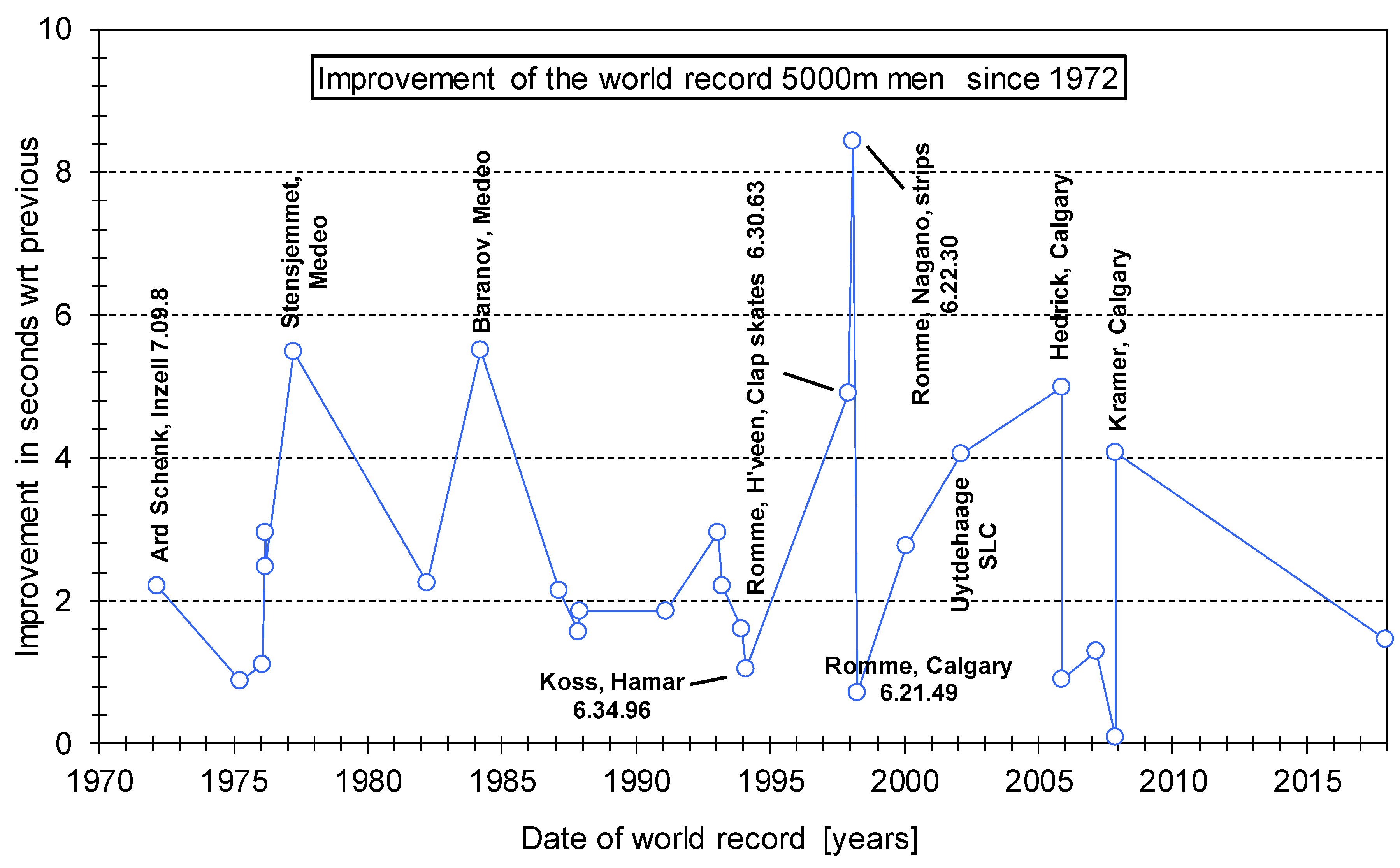
Figure 10 presents a historical overview of the improvements of the world record on the men’s 5000 m since 1972. Depicted is the improvement in seconds with respect to the previous record, starting with the 1972 world record of Ard Schenk in Inzell, a German medium-altitude (690 m.) outdoors skating rink. The figure shows a top seven of improvements better than 4 s. Clearly visible are the records set at the 1691 m altitude Medeo natural ice rink in Almaty, Kazachstan, with its sometimes favorable wind. Two others were set by Gianni Romme, one showing the advantage of the clap skates introduced in the season 1996–1997 and one with both the clap skates and the zigzag strips including the advantage of the low ambient pressure during the Olympic race. The record of Uytdehaage might be associated with the introduction of the Nike Swift skinsuit at the 2002 Salt Lake City Winter Olympics. The improvement of Romme is the second largest since the beginning of the 20th century, only topped by Boris Shilkov, in 1955, who skated at the Medeo magic oval (18.1 s).
In 
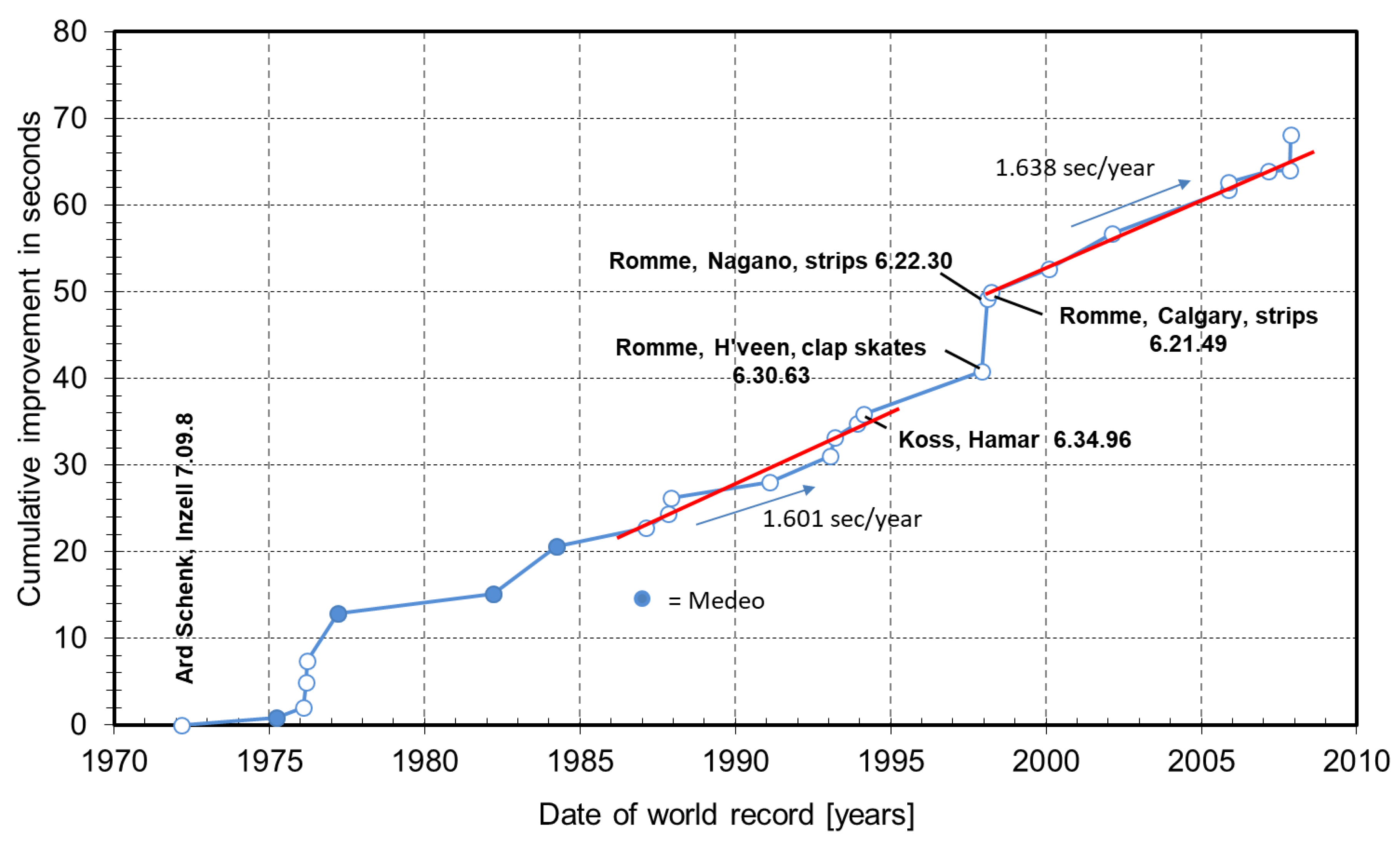
Figure 11, all of these incremental changes are put together, again with the starting point in 1972. The coordinates for the horizontal axis were computed according to the dates the records were skated: 15 February 1995 is 1995.126. The graph nicely depicts the development of the men’s 5000 m world record during the last four decades. Over the years, many factors have contributed to higher skating speeds—some in a gradual way, like improvements in nutrition, training methods (better understanding of the skating technique) and medical support; some in a small jump, such as the erection of indoor skating rinks and the associated ice preparation; and others in a more abrupt way, such as innovations in skates and suits. If specific performance improvements follow an S-curve, Figure 11 can be seen as the sum of a continuous stream of S-curves with smaller or larger jumps on top of a generally increasing curve associated with learning and societal wellbeing.
An abrupt change is clearly visible around 1976 and might be associated with the introduction of the skinsuit one year earlier. By 1976, all the skaters wore the tightly fitting Lycra suit, and, over one year (including the Olympic Games of Innsbruck), lap times improved with an average of 0.52 s. The increase in speed around 1987 can be traced back to the opening of the indoor rinks of Heerenveen and Calgary. The average improvement of the world record in the 10 years prior to the introduction of the clap skate in 1996/97 is 1.601 s per year (R2 = 0.935), or 0.128 s per lap per year. In the ten years after the introduction of the zigzag strips on the suit, 1998–2008, the average improvement slightly increased to 1.638 s per year (R2 = 0.965), resulting in a 0.131 s per year decrease in lap time, albeit that the level is more than 8 s higher than before.
After Jan Olav Koss set the record on conventional skates during the Olympic Games in Hamar, Norway, it took about 3.5 years until the introduction of the clap skate before the record was broken again. Such long periods usually occur when innovations have reached the end of their development curve. The jump around 1997 and 1998 can be associated with the introduction of the clap skate and the zigzag strips. Since there was no 5000 m world record set just before the introduction of the clap skate, it is a bit hard to distinguish the two in terms of contribution to the improvement of lap times.

5.3.2. Results for 1500 m

A more detailed analysis is possible when we look at the development of the 1500 m world record presented in Figure 12 with data from Reference [22]. The figure shows an average improvement of 0.196 s/year (R2 = 0.937) in the period 1984–1996 prior to the introduction of the clap skate, a large jump in the years of the introduction of the clap skate and the zigzag strips and an average improvement of 0.437 s per year (R2 = 0.974) in the following 10 years.
To unravel the respective contributions of clap skate and zigzag strips, let us start with the March 1996 world record of the Japanese Hiroyuki Noake in Calgary, the last on conventional skates. In March 1998, two years later, also in Calgary, the world record was 4.18 s faster. Of the 4.18 s, 3.52 s was realized in approximately one year (starting with Marshall on 16 March 1997) and 2.64 s (Overland, November 1997) in the four months prior to Søndrål’s Calgary world record with drag-reducing strips. After the introduction of the zigzag devices in the first race of the Nagano Olympic speed-skating races, the 5000 m, Søndrål adopted the zigzag strips and used them in his world-record race on the 1500 m, in Nagano as well. The world record of Ritsma (December 1997, Heerenveen) was the last skated with clap skates but without aerodynamic changes to the suit at a low-land track. His record was 1.73 s faster than Noake’s, but without the bonus of skating on a high altitude rink such as Calgary. In this respect, the Calgary track record of Dutchman Jan Bos may be of value, since this was skated on November 28 1997. His time of 1:48.68 (1.93 s faster than Noake) was not a world record, due to the unofficial status of his participation in the Canada–USA international speed-skating match. Bos was the last to skate on the Olympic Oval, breaking the world’s fastest time on the 1500 m with clap skate but without improved aerodynamics. Taking into account the average of 0.20 s per year reduction of the 1500 m times, which could be realized irrespective of significant technology influences, it seems that about 2.20 s of the resulting 3.78 s gain on Noake’s 1500 m world-record time of 1996 may be attributed to improved performance due to the zigzag strips, which means an approximate 0.59 s gain per lap. Note that, due to the clap skate coming of age but presumably more propelled by research into further aerodynamic drag reduction, in the decade following 1998, race-time improvement per year more than doubled.

6. The Effect of Zigzag Tape Relative to Rough Fabrics

In November 2007, the International Skating Union (ISU) banned devices that were not an integral part of the suit, resulting in the separate zigzag strips not being allowed anymore. Long before that, the role of triggering transition on the lower legs was taken over by rough fabrics, which are also more suited for the upper legs and arms, as these undergo much more angle-of-attack changes during skating. Until the decision of the ISU, some teams chose a hybrid solution: using zigzag tape on the cap, for the reasons mentioned in Section 3.3.2. During post-Nagano wind-tunnel campaigns, besides the effect of zigzag strips, the drag-reducing effect of various types of fabrics were also investigated. Figure 13 depicts the zigzag tape results relative to the effect of fabrics with different roughness measured on a two-dimensional cylinder. Both applications aim at reducing the aerodynamic drag but showing some different flow behavior. It appears that the zigzag tape does not give the lowest drag but stays at a low Cd-value for quite a range in Reynolds numbers, due to the fact that it partly works as a row of vortex generators. The vortices emanating from the tape mix higher momentum air at a larger distance from the surface with the lower part of the boundary layer, energizing it and enabling it to stay attached to the surface much longer than simple roughness can do.
The use of fabrics with a certain roughness may lead to a lower drag coefficient in the right Reynolds number range, but it also may result in a much higher drag in an off-design condition. An example is given in Table 6, where the Reynolds number is calculated for two ice rinks with extremities in altitude: Thialf, in Heerenveen, at sea level; and the Utah Olympic Oval, in Salt Lake City, at 1423 m elevation. The average speed was calculated from the track records; the barometric pressure was taken from standard atmosphere tables. At a high-altitude track, the rink temperature may be the same, but the barometric pressure is, of course, much lower. As a result, at altitude, the kinematic viscosity, ν (=µ/ρ), is higher, and the Reynolds number of a leg (here based on an estimated total leg average equivalent diameter) is lower.
The leg of a skater having the optimum roughness with fabric 2 around a Reynolds number of 1.21 × 10⁵ in Heerenveen may experience a serious drag increase when moving to a high-altitude track such as Salt Lake City, despite the higher speed (Re = 1.04 × 10⁵). For the cylinder in Figure 13, the drag due to the change in Reynolds number is increased with more than 50%. If the aerodynamics of the leg follow the cylinder trend, this means the designer has to stay on the safe side by choosing a fabric that has its lowest drag at a lower Reynolds number than fabric 2, unfortunately, overall, at a higher drag level. With zigzag tape, the change in drag would be very small. Table 7 presents the extremities in the Reynolds number now based on the highest speed for men (1000 m race) at sea level and the lowest speed for women at high altitude (5000 m race), again on the basis of average speeds of present-day track records. In combination with Figure 13, it shows that it is not a good idea to use the same fabric for women and men at every altitude and distance.
A further decrease of the suit drag when using rough fabrics can only be accomplished by further personalizing the fabrics, closely looking at the various Reynolds numbers of the particular body parts at the various distances and altitudes. Figure 13 clearly shows that the zigzag strips can safely be used over a large range of Reynolds numbers, albeit at a somewhat smaller reduction in aerodynamic drag than achieved by using dedicated fabrics. Hence, as separate zigzag strips are not allowed anymore, it may be interesting to investigate whether the efficient vortex-producing effect of the zigzag strips can be obtained by a new type of fabric within the ISU regulations.

7. Conclusions

From a comparison of the race times Gianni Romme and his Dutch and International competitors realized at three consecutive 5000 m races around the 1998 Nagano Winter Games, where Romme came out as the winner, the impact of zigzag strips on lower legs and cap was established to be between −4.2% and −5.3% on drag area. Translated to a 5000 m race at sea level with the 1998 average speeds, this is an improvement of 0.42 to 0.53 s per lap.
An analysis of historic 1500 m men’s speed-skating world-record times showed an advantage of the zigzag tape of 0.59 s per lap on the 1500 m.
Overall, an improvement of 0.5 s in lap times for male speed skaters may have been realized by using zigzag strips.
Looking at the differences in Reynolds numbers of the lower legs of female and male speed skaters, to further decrease the drag by using race suits, they should be personalized regarding aerodynamically efficient fabrics and even be made rink/altitude dependent.
In retrospect, the introduction of the zigzag tape technology and the apparent reduced drag put the aerodynamics of speed skaters on the research charts again. It was the first big step in a still ongoing process to reduce speed skater drag by aerodynamically efficient race suits.

Author Contributions

Regarding the presented wind-tunnel results and application of the zigzag devices: conceptualization, methodology, validation and formal analysis, N.T. and L.V. Regarding the present paper: investigation of actual zigzag tape performance improvement and original draft preparation, N.T.; review and editing, L.V. All authors have read and agreed to the published version of the manuscript.

Funding

This research received no external funding.

Institutional Review Board Statement

The Institutional Review Board at Delft University of Technology called HREC (Human Resource Ethics Committee) was not installed yet in the year 1997 when the experiments on live speed skaters were performed. As such a signed statement cannot be provided. However, based on the type of measurements reported herein combined with the fact that no non-trivial actions were required from the skaters other than taking a natural speedskating posture inside the wind tunnel, it should be clear that no forceful attempt was made to ask the skaters to act outside their comfort zone. All skaters volunteered to act as wind tunnel model throughout the measurement campaign. Moreover, the authors do not have evidence that unlawful pressure was put on the speed skaters by their employer to join the tests.

Informed Consent Statement

Informed consent was obtained from all subjects involved in the study, with the exception of chapter 5, which is entirely based on publicly available information.

Data Availability Statement

Upon request data can be obtained from the authors.

Conflicts of Interest

The authors declare no conflict of interest.

References

  1. De Koning, J.J. World Records: How Much Athlete? How Much Technology? Int. J. Sports Physiol. Perform. 2010, 5, 262–267. [Google Scholar] [CrossRef] [PubMed] [Green Version]
  2. Oggiano, L.; Brownlie, L.; Troynikov, O.; Bardal, L.M.; Sæter, C.; Sætran, L. A Review on Skin Suits and Sport Garment Aerodynamics: Guidelines and State of the Art. Procedia Eng. 2013, 60, 91–98. [Google Scholar] [CrossRef] [Green Version]
  3. Brownlie, L.W.; Kyle, C.R.; Harber, E.; MacDonald, R.; Shorten, M. Reducing the aerodynamic drag of sports apparel: Development of the NIKE Swift sprint running and SwiftSkin speed skating suits. In The Engineering of Sport 5; Hubbard, M., Mehta, R., Pallis, J., Eds.; ISEA: Sheffield, UK, 2004. [Google Scholar]
  4. Dobbinga, E. The Effect of Trip Wires on the Drag of Speed Skaters; Memorandum M-583, (Report Based on an Internal Technical Note LSW 84-2 from April 1984); Faculty of Aerospace Engineering, Delft University of Technology: Delft, The Netherlands, November 1987. (In Dutch) [Google Scholar]
  5. Veldhuis, L.L.M.; Timmer, W.A. Investigation into the Aerodynamic Drag of a Skater Using an Experimental One-Component Strain-Gauge Balance; Internal report LSW 97-3; Faculty of Aerospace Engineering and Institute for Wind Energy, Delft University of Technology: Delft, The Netherlands, July 1997. (In Dutch) [Google Scholar]
  6. Timmer, W.A.; Veldhuis, L.L.M. Further Research into the Possible Application of Zigzag Strips on Speed Skaters; Report IW-98138R; Institute for Wind Energy, Delft University of Technology: Delft, The Netherlands, July 1998. (In Dutch) [Google Scholar]
  7. Timmer, W.A.; Postma, I. Everything about Strips. Speed Skating World, Postma, I., Ed.; The Netherlands, September 1998; Issue 8, 23–25. [Google Scholar]
  8. Timmer, W.A. Fast Suits, New Archive of Mathematics NAW 5/5 nr. 4; Mathematics Institute, University of Leiden: Leiden, The Netherlands, December 2004; pp. 292–295. (In Dutch) [Google Scholar]
  9. Fage, A.; Warsap, J.H. The Effects of Turbulence and Surface Roughness on the Drag of a Cylinder; ARC RM 1283; H.M. Stationery Office: London, UK, 1929. [Google Scholar]
  10. Hoerner, S.F. (Ed.) Fluid Dynamic Drag; Bakersfield, CA, USA, 1965. [Google Scholar]
  11. Ewald, B.F.R. (Ed.) Wind Tunnel Wall Corrections, AGARD AG-336; North Atlantic Treaty Organization: Brussels, Belgium, October 1998. [Google Scholar]
  12. De Koning, J.J. Faculty of Human Movement Sciences; VU University Amsterdam, Personal Communication: Amsterdam, The Netherlands, August 2009. [Google Scholar]
  13. Schenau, G.V.I. The influence of air friction in speed skating. J. Biomech. 1982, 15, 449–458. [Google Scholar] [CrossRef]
  14. Available online: www.sports-reference.com/olympics/athletes (accessed on 12 March 2018).
  15. De Koning, J.J.; De Groot, G.; Schenau, G.J.V.I. Ice friction during speed skating. J. Biomech. 1992, 25, 565–571. [Google Scholar] [CrossRef]
  16. Weather Underground. Available online: www.wunderground.com/history (accessed on 17 December 2020).
  17. Shinano Mainichi Shimbun Inc. Official Report of the XVIII Olympic Winter Games Vol. III, Competition Results and Partici-Pants; 1998 (NAOC); The Organizing Committee for the XVIII Olympic Winter Games: Nagano, Japan, 1999. [Google Scholar]
  18. Van Ingen Schenau, G.J.; de Koning, J.J.; de Groot, G. A simulation of speed skating performances based on a power equation. Med. Sci. Sports Exerc. 1990, 22, 718–728. [Google Scholar] [CrossRef] [PubMed]
  19. Van Erck, D.; Wenker, E.J.; Levels, K.; Foster, C.; De Koning, J.J.; Noordhof, D.A. Cycling at Altitude: Lower Absolute Power Output as the Main Cause of Lower Gross Efficiency. Int. J. Sports Physiol. Perform. 2019, 14, 1117–1123. [Google Scholar] [CrossRef] [PubMed]
  20. Noordhof, D.A.; Mulder, R.C.M.; de Koning, J.J.; Hopkins, W.G. Race Factors Affecting Performance Times in Elite Long-Track Speed Skating. Int. J. Sports Physiol. Perform 2016, 11, 535–542. [Google Scholar] [CrossRef] [PubMed]
  21. Muehlbauer, T.; Schindler, C.; Panzer, S. Pacing and sprint performance in speed skating during a competitive season. Int. J. Sports Physiol. Perform. 2010, 5, 165–176. [Google Scholar] [CrossRef] [PubMed] [Green Version]
  22. SpeedSkatingStats. Available online: www.SpeedSkatingStats.com (accessed on 17 December 2020).
Figure 1. The foam zigzag tape for the lower legs and cap introduced at the 1998 Nagano Olympics.
Applsci 11 00988 g001
Figure 2. Fluorescent oil flow visualization of the effect of zigzag tape on the separation location on the lower leg. The flow comes from the right. Zigzag-tape thickness in right picture is 0.93 mm.
Applsci 11 00988 g002
Figure 3. Setup of a 90 cm span circular cylinder in the Delft University low-speed, low-turbulence wind tunnel. In this case, the aerodynamic characteristics of a fabric with small rubber triangles were determined. The diameter of the cylinder is 11 cm.
Applsci 11 00988 g003
Figure 4. The impact of zigzag tape location on the drag coefficient of a smooth cylinder. Tape on the left and the right from the leading edge. Tape thickness is 0.93 mm; cylinder span is 60 cm.
Applsci 11 00988 g004
Figure 5. The effect of zigzag tape thickness on the drag coefficient of a cylinder. Tape at an azimuth position of 30° on the left and right from the leading edge. Cylinder span is 60 cm. If not indicated otherwise, the zigzag tape used during all measurements has the layout of the Teflon tape shown in the insert.
Applsci 11 00988 g005
Figure 6. The drag variation with angle of attack of a small mannequin leg covered with a smooth skinsuit and 0.93 mm thick zigzag tape on the lower leg, at an azimuth angle of 55 degrees. Re = 0.73 × 10⁵. The measurements presented here were performed in the configuration of Figure 2, i.e., without the table and the skate.
Applsci 11 00988 g006
Figure 7. The test setup of the measurements on live skaters in January 1997.
Applsci 11 00988 g007
Figure 8. The effect of zigzag tape on the lower legs and cap of a male long-distance speed skater’s drag area at a wind speed of 12.1 m/s. RD = 0.8 × 10⁵ (based on lower-leg average equivalent diameter). Tape at 55° equivalent azimuth angle for five sequential test runs.
Applsci 11 00988 g008
Figure 9. The average reduction in power output with simulated altitude of 21 male trained cyclists performing a 4000 m time trial [19].
Applsci 11 00988 g009
Figure 10. Incremental improvement in seconds of the 5000 m world record since 1972.
Applsci 11 00988 g010
Figure 11. Cumulative improvement of the 5000 m world record since 1972.
Applsci 11 00988 g011
Figure 12. Cumulative improvement in seconds of the 1500 m world record for men since 1976.
Applsci 11 00988 g012
Figure 13. The impact of zigzag tape and rough fabrics on the drag coefficient of a circular cylinder. Nagano foam zigzag tape t = 1.2 mm, at an azimuth of 45 degrees. Cylinder span, 90 cm.
Applsci 11 00988 g013
Table 1. Averages over five runs of the drag area CDA of three configurations showing the effect of 0.5 mm thick zigzag tape on lower legs and 0.75 mm on the cap.
ConfigurationCDAσ (%)
Standard suit, no tape, series 10.2550.7
Standard suit, zigzag tape on lower legs0.2331.9
Standard suit, no tape, series 20.2551.7
Standard suit, zigzag tape on cap0.2448.1
Table 2. Parameters to calculate the Reynolds number range of the lower legs.
Leg LocationDistance1997 WR Vaverage (m/s)±ΔV (m/s)Deq (m) Reav±ΔRe±ΔRe (%)
Calf1500 m1.48.8813.782.60.1251.18 × 1050.22 × 10519
Ankle1500 m1.48.8813.7840.0690.65 × 1050.19 × 10529
Calf5000 m6.30.6312.82.60.1251.09 × 1050.22 × 10520
Ankle5000 m6.30.6312.840.0690.60 × 1050.19 × 10531
Table 3. Calculation of Romme’s average power output in Heerenveen 1997 and Calgary 1998.
LocationT (°C)Pbar (hPa)ρ (kg/m3)µg (m/s2)TimeCDAVavg (m/s)Preq (W)
Heerenveen1310121.2320.0049.8066:30.630.27512.800398
Calgary13890 **1.0840.0049.8046:21.490.275 *13.107379
* Without drag-reducing devices, ** including 7 hPa for 65 m height difference airport ice rink.
Table 4. The calculated drag area of Gianni Romme in Nagano and Calgary with his estimated power available at altitude, using a power loss factor of 0.923 per 1000 m elevation. Local barometric pressures were used; h-cor is the corrected elevation according to the ISA standard.
LocationT (°C)Pbar (hPa)ρ (kg/m3)h-cor (m)Loss Factor (-)P (W)Vavg (m/s)CDAImprovement (%)
Heerenveen1310121.23200397.912.8000.27500
Nagano139511.1585400.958381.213.0820.26055.27
Calgary138901.08410800.917364.913.1070.26344.22
Table 5. Differences with Romme of a number of elite skaters at three consecutive 5000 m races.
Ranking Seconds behind Romme in
CalgaryNameCountryHeerenveenNaganoCalgary
1Gianni RommeNED00 *0 *
2Rintje RitsmaNED5.36 *4 *
3Bart VeldkampBEL-6.1 *6.1 *
4Remi HereideNOR6.817.57.4 *
5Bob de JongNED39.2 *8.1 *
6Frank DittrichGER7.9128.6 *
7Roberto SighelITA11.115.99.1 *
8Steven ElmCAN18.626.511.3 *
* With zigzag strips.
Table 6. The effect of altitude on the lower-leg average Reynolds number, men’s 5000 m.
LocationAlt.TPbarνDeqVavgRe
(m)(°C)(hPa)(m2/s)(m)(m/s)
Heerenveen0131013.31.461 × 10−50.1313.58 *1.21 × 105
Salt Lake City142313853.61.734 × 10−50.1313.82 **1.04 × 10⁵
* Final time of 6:08.21; ** final time of 6:01.86.
Table 7. Extremities in lower-leg Reynolds number, following from track records for male and female skaters.
LocationAlt. (m)T (°C)Pbar (hPa)ν (m2/s)Deq (m)Vavg (m/s)Re
Heerenveen
1000 m Men
0131013.31.461 × 10−50.1314.90 *1.32 × 105
Salt Lake City
5000 m Women
142313853.61.734 × 10−50.1212.44 **0.86 × 10⁵
* Final time of 1:07.09, ** final time of 6:42.01.
Publisher’s Note: MDPI stays neutral with regard to jurisdictional claims in published maps and institutional affiliations.

