Article

Consistency Analysis and Accuracy Assessment of Eight Global Forest Datasets over Myanmar

1
School of Surveying and Geo-Informatics, Shandong Jianzhu University, Jinan 250101, China
2
Land Spatial Data and Remote Sensing Technology Institute of Shandong Province, Jinan 250002, China
3
School of Geosciences and Info-Physics, Central South University, Changsha 410083, China
4
Faculty of Geography, Yunnan Normal University, Kunming 650500, China
*
Author to whom correspondence should be addressed.
Appl. Sci. 2021, 11(23), 11348; https://doi.org/10.3390/app112311348
Submission received: 11 November 2021 / Revised: 24 November 2021 / Accepted: 25 November 2021 / Published: 30 November 2021

Abstract

:
Accurate and up-to-date forest monitoring plays a significant role in the country’s society and economy. Many open-access global forest datasets can be used to analyze the forest profile of countries around the world. However, discrepancies exist among these forest datasets due to their specific classification systems, methodologies, and remote sensing data sources, which makes end-users difficult to select an appropriate dataset in different regions. This study aims to explore the accuracy, consistency, and discrepancies of eight widely-used forest datasets in Myanmar, including Hansen2010, CCI-LC2015, FROM-GLC2015/2017, FROM-GLC10, GLC-FCS2015/2020, and GlobeLand30-2020. Firstly, accuracy assessment is conducted by using 934 forest and non-forest samples with four different years. Then, spatial consistency of these eight datasets is compared in area and spatial distribution. Finally, the factors influencing the spatial consistency are analyzed from the aspects of terrain and climate. The results indicate that in Myanmar the forest area derived from GlobeLand30 has the best accuracy, followed by FROM-GLC10 and FROM-GLC2017. The eight datasets differ in spatial detail, with the mountains of northern Myanmar having the highest consistency and the seaward areas of southwestern Myanmar having the highest inconsistency, such as Rakhine and the Ayeyarwady. In addition, it is found that the spatial consistency of the eight datasets is closely related to the terrain and climate. The highest consistency among the eight datasets is found in the range of 1000–3500 m above sea level and 26°–35° slope. In the subtropical highland climate (Cwb) zone, the percentage of complete consistency among the eight datasets is as high as 60.62%, which is the highest consistency among the six climatic zones in Myanmar. Therefore, forest mapping in Myanmar should devote more effort to low topography, seaward areas such as border states like Rakhine, Irrawaddy, Yangon, and Mon. This is because these areas have complex and diverse landscape types and are prone to confusion between forest types (e.g., grassland, shrub, and cropland). The approach can also be applied to other countries, which will help scholars to select the most suitable forest datasets in different regions for analysis, thus providing recommendations for relevant forest policies and planning in different countries.

1. Introduction

Forest is the dominant component of the earth’s biogeochemical system, which provides critical refuge for terrestrial biodiversity [1,2]. Accurate and up-to-date forest cover information is considered an important parameter to help humans to protect, conserve, monitor, and sustainably manage forests and ensure their ecological functions [3]. As one of the most forested tropical countries in mainland Southeast Asia [4], forest cover is particularly important in Myanmar. This is because forests in Myanmar support many important and endemic species of great value to global biodiversity conservation [5], and play a significant social and economic role in the country [6]. Due to its rapid socio-economic development, Myanmar is facing a critical situation with severe deforestation [7]. Therefore, it is necessary to conduct forest mapping regularly to monitor forest cover and its changes in Myanmar.
Satellite remote sensing technology is widely used for forest mapping and monitoring [8,9,10]. Currently, many land cover datasets have been produced with different spatial and temporal resolutions. Since the earliest 1 km resolution UMD [11] and IGBP [12,13] were derived, many other land cover maps have been produced, such as the 1 km Global Land Cover 2000 (GLC2000) [14] and 500 m MODIS Land Cover dataset [15,16]. The advent of medium-resolution satellites has facilitated the emergence of datasets with higher spatial resolution such as GlobCover [17,18] and European Space Agency Climate Change Initiative Land Cover (CCI-LC) products [19], which have a resolution of 300 m. The Finer Resolution Observation and Monitoring Global LC(FROM-GLC) dataset [20,21] and GlobeLand30 [22] both reach a spatial resolution of 30 m representing significant advances. Furthermore, now the resolution of the land cover dataset FROM-GLC10 has reached 10 m [23]. There must be some discrepancies among these datasets due to their different production purposes, satellite data sources, classification systems, and methods [24,25,26], which make it difficult for end-users to select an appropriate dataset.
To help end-users to select their specific forest datasets, this study aims to evaluate the accuracy, consistency, and discrepancies of eight forest datasets in Myanmar (i.e., Hansen2010, CCI-LC2015, FROM-GLC2015/2017, FROM-GLC10, GLC-FCS2015/2020, and GlobeLand30-2020). Specifically, (1) we provide accuracy assessment by comparison with sample points collected from multi-temporal high-resolution images on Google Earth (GE); (2) we compare the area and spatial agreement among different datasets; (3) we explore the driving factor within the two recognized impacting factors (i.e., terrain and climate) over the discrepant areas.
The following section describes global land cover datasets and ancillary data for assessment, together with the overall methodology. Section 3 presents the results of the study in terms of the accuracy and comparison of forest categories in different datasets, with the limiting factors. Section 4 discusses the reasons for the discrepancy between datasets and the future directions for improvement. Finally, Section 5 summarizes the research significance and findings of the paper, as well as the challenges and suggestions for future forest mapping.

2. Materials and Methods

2.1. Global Land Cover Datasets
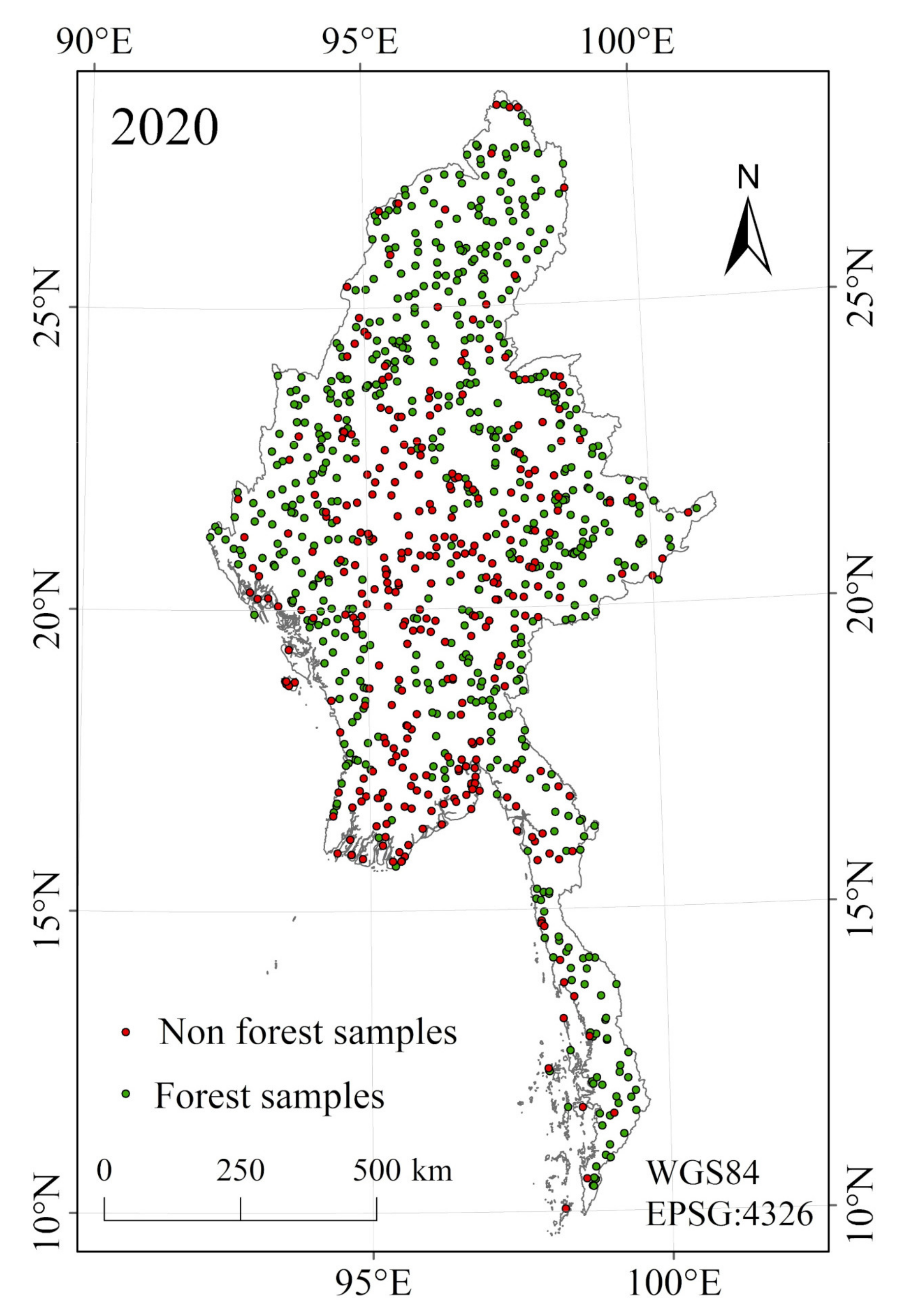
The detailed information of used land cover datasets is summarized and shown in Table 1.
The Hansen 2010 Global Forest Cover Dataset was developed in collaboration with the GLAD (Global Land Analysis and Discovery) Laboratory at the University of Maryland, Google, the U.S. Geological Survey, and NASA [27]. It used clear surface observations from more than 600,000 images analyzed by Google Earth Engine (a cloud-based platform for earth observation and data analysis). The tree coverage per pixel was determined using supervised learning algorithms [28].
The ESA’s Land Cover (LC-CCI) project, built on the experience of the GlobCover, delivered four consecutive GLC maps for five-year epochs centered around 2000, 2005, 2010, and 2015, with a spatial resolution of 300 m [19]. The product has a fine-grained classification system, with a legend based on LCCS with 22 classes, which is more suitable for large-scale, long-time series land cover change studies.
GLC-FCS has two datasets of different years. The first version became available in 2015. It is based on location information from the image spectral library and the time-series Landsat8 surface reflectance product, combined with a multi-temporal classification model and a time-series reflectance dataset [29]. On this basis, GLC-FCS30-2020 has been produced, combining the 2019–2020 time-series Landsat surface reflectance data, Sentinel-1SAR data, DEM, global thematic auxiliary datasets, and a priori knowledge datasets [30]. The dataset contains a total of 30 types of land cover information for global terrestrial regions. However, the secondary forest classes (dense and open) in 2015 are only reflected in some local areas, and remain indistinguishable in most global regions, including Myanmar. This problem is effectively improved in 2020.
FROM-GLC is the first 30 m resolution global land cover map by using a support vector machine classifier from Landsat imagery [20,21]. Later, the world’s first 10 m resolution global land cover product, FROM-GLC10, was released in 2019. Compared with FROM-GLC30, which has a 30 m resolution, it provides more spatial details. In terms of the classification system, FROM-GLC2015 produced to the secondary category, its forest was subdivided into 6 subcategories. FROM-GLC2017 and FROM-GLC10 focused on the primary category, and different types of tree species all corresponded to “forest”.
GlobeLand30 of the National Geomatics Centre of China (NGCC) was developed using a pixel-object-knowledge (POK) to derive a global land cover map at 30 m resolution by multispectral images [22]. The 2020 version also used GF-1 multispectral images with 16 m resolution. Its classification system included ten land cover types, with forests as one of them.

2.2. Auxiliary Data

To objectively perform an accuracy assessment, we used 934 randomly selected forest and non-forest samples, which were collected via visual interpretation of high-resolution images on GE for four years (i.e., 2010, 2015, 2017, and 2020). Based on the overlay of the consistency distribution maps of the eight datasets, 747 sample points were obtained by random sampling at different consistency levels at 0.01%, the remaining samples were from the Global validation sample set [31]. The spatial distribution of the validation samples is shown in Figure 1.
To analyze the driving factors for spatial consistency from the aspects of terrain and climate, we chose (1) the Digital Elevation Model (DEM) data with 30 m resolution from Shuttle Radar Topography Mission (SRTM) [32,33] and calculated the slope data based on it; (2) KÖPPEN-Geiger climate classification [34] scheme includes six climate zones in Myanmar (Figure 2): Tropical Monsoon Climate (Am), Tropical Savanna Climate (Aw), Humid Subtropical Climate (Cwa), Subtropical Highland Climate (Cwb), Sub-boreal Monsoon Climate (Dwc) and Boreal Tundra Climate (ET).

2.3. Forest Data Harmonization for Comparison and Analysis

Data harmonization is a key step to ensure the objectivity of the comparison among different datasets. In this study, data harmonization included two steps, i.e., spatial resolution unification and legend harmonization. First, land cover datasets and DEM data were resampled to 300 m resolution by using the nearest neighbor method to match with the coarse-resolution product (CCI-LC). Then, legend harmonization was performed before comparison, because each dataset defined forest differently and according to different descriptors [35,36]. The Hansen Global Forest Cover Dataset contains only forest land classes, and the classification systems of the other seven datasets on forests need to be combined. CCI-LC and GLC-FCS have more secondary classes and their classification system is the Land cover classification system (LCCS) scheme. In this paper, we carried out the unification of forest land classes of these two datasets according to the Intergovernmental Panel on Climate Change (IPCC) standards. FROM-GLC and GlobeLand30 only need to extract or merge (FROM-GLC2015) the forest land classes according to the data description. The specific forest land class conversion rules are shown in Table 2, and the spatial distribution data of Myanmar forests extracted from each dataset is shown in Figure 3. We chose to simplify the classification because detailed land cover type diversification may create more uncertainty [37].
To evaluate the spatial consistency among the eight products, we overlaid all forest cover datasets to obtain a spatial consistency distribution map. Different consistency levels were indicated by the magnitude of consistency. The consistency degree is divided into eight levels, “8” indicates that the eight datasets on the pixel are the same, and the pixel is judged to be a forest type. In this way, “1” indicates the worst consistency condition, i.e., only one dataset classifies the pixel as a forest type. In addition, to reduce the influence of the time factor, we also selected three different datasets for 2015, i.e., CCI-LC, FROM-GLC, and GLC-FCS, and performed spatial consistency analysis for these three datasets, whose consistency levels correspond to a total of three levels.
To explore the spatial pattern of the disagreement and its potential causes, we further analyzed the relationship of spatial consistency with terrain and climate. The landscape forms are divided into five types according to elevation: plain (<200 m), hilly (200~500 m), low mountain (500~1000 m), medium mountain (1000~3500 m), and high mountain (>3500 m). Meanwhile, the slope is divided into six classes according to the forestry slope class plan, i.e., flat slope (≤5°), gentle slope (6°~15°), slope (16°~25°), steep slope (26°~35°), sharp slope (36°~45°) and dangerous slope (≥46°). We calculated the spatial consistency among different elevation and slope zones, and overlapped the climate distribution on the consistency, then calculated it within each of the six climate zones.

3. Results

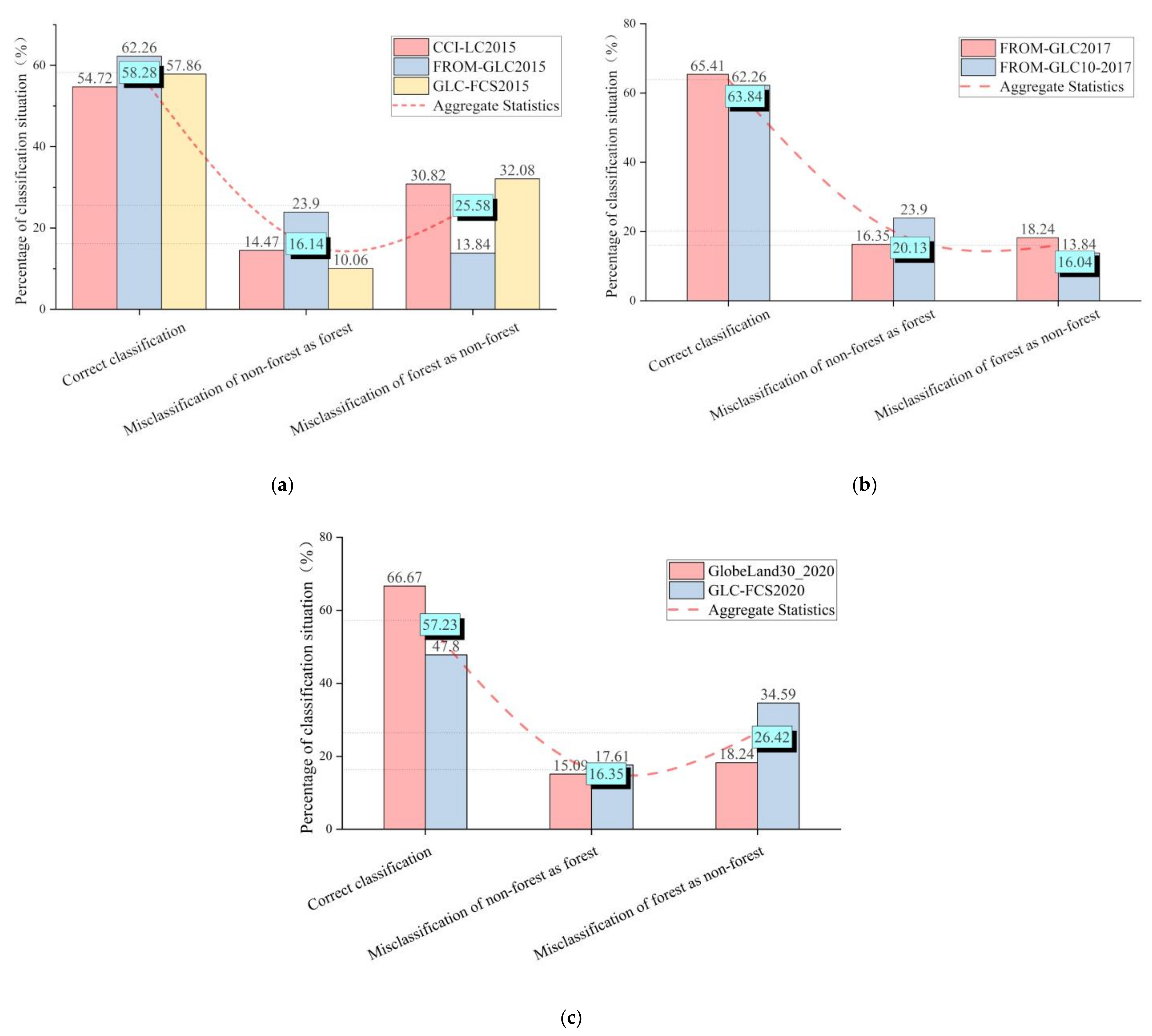
3.1. Accuracy Assessments

Table 3 shows the confusion matrix for the eight forest datasets. The FROM-GLC10 dataset in 2017 has the best accuracy, with an overall accuracy (OA) of 84.48% and a Kappa of 0.65. Followed by FROM-GLC2017 with 30 m resolution and the GlobeLand30, they both have an overall accuracy of 83.51%. The OA of the Hansen2010 and the FROM-GLC2015 both exceed 80%. In contrast, CCI-LC and GLC-FCS have lower accuracy for the forest. Specifically, the GLC-FCS has a high misclassification rate on non-forest. In both years of GLC-FCS, the user precision of non-forest is 60.92% and 60.96%, respectively. Meanwhile, it has a relatively high percentage of omission of 31.81% for forests in 2015. This percentage improves in 2020, which decreases to 25.74%. The CCI-LC has a high percentage of misclassification of 34.32% for non-forest and an omission of 26.71% for the forest.
Although the OA and Kappa of FROM-GLC10 are the highest among the eight datasets, it has a lower mapping accuracy of 69.16% in non-forest. It means that there is a higher possibility of omission in non-forest, i.e., there is a large amount of overestimation in forests. In comparison, the OA and Kappa of the FROM-GLC2017 with 30 m resolution and GlobeLand30 are slightly lower, but their user precision and mapping accuracy are more stable. In the classification of forests, the misclassification and omission of GlobeLand30 are slightly better than the FROM-GLC. Therefore, GlobeLand30 is the best dataset in terms of the production of forest classification.

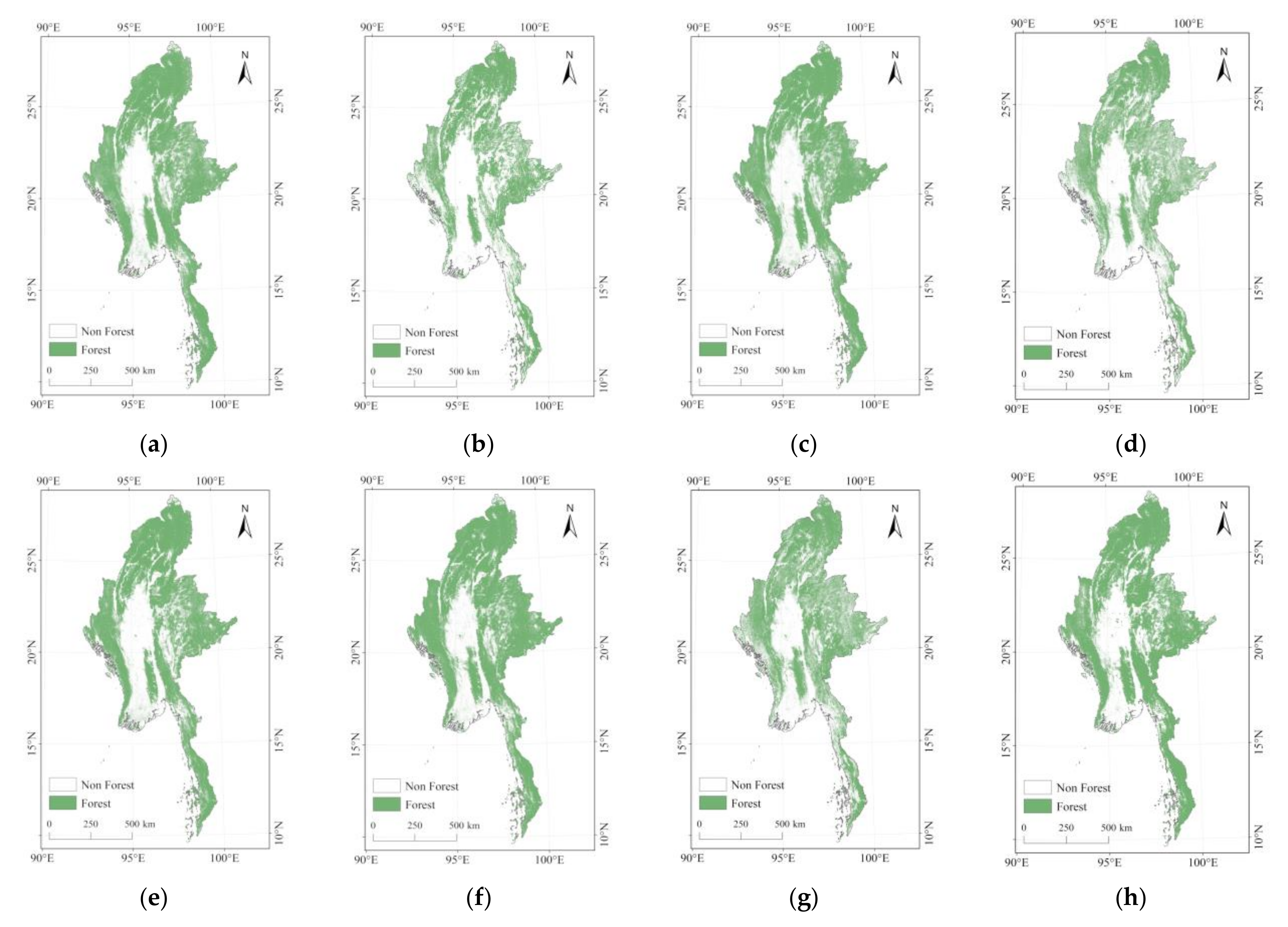
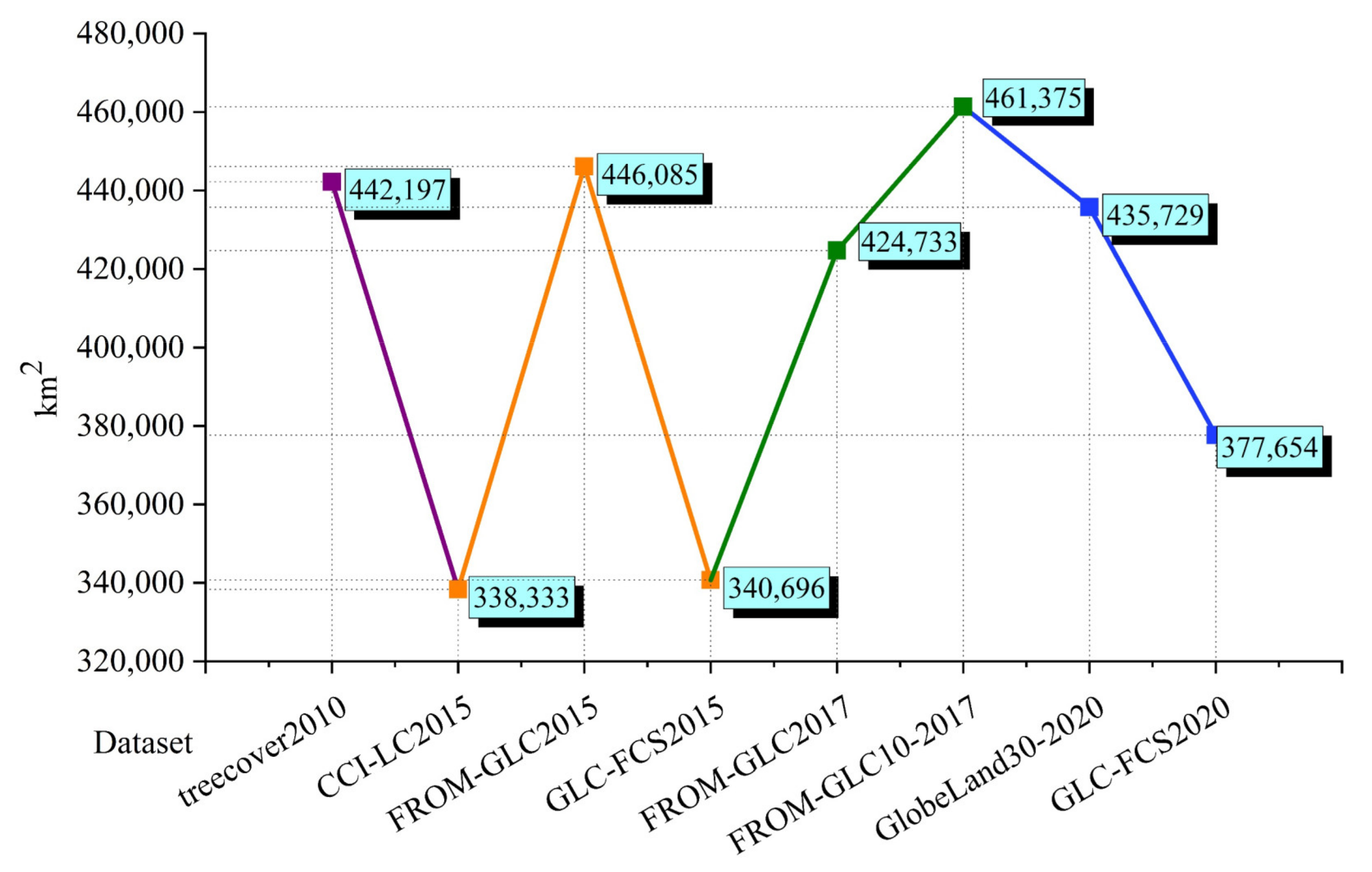
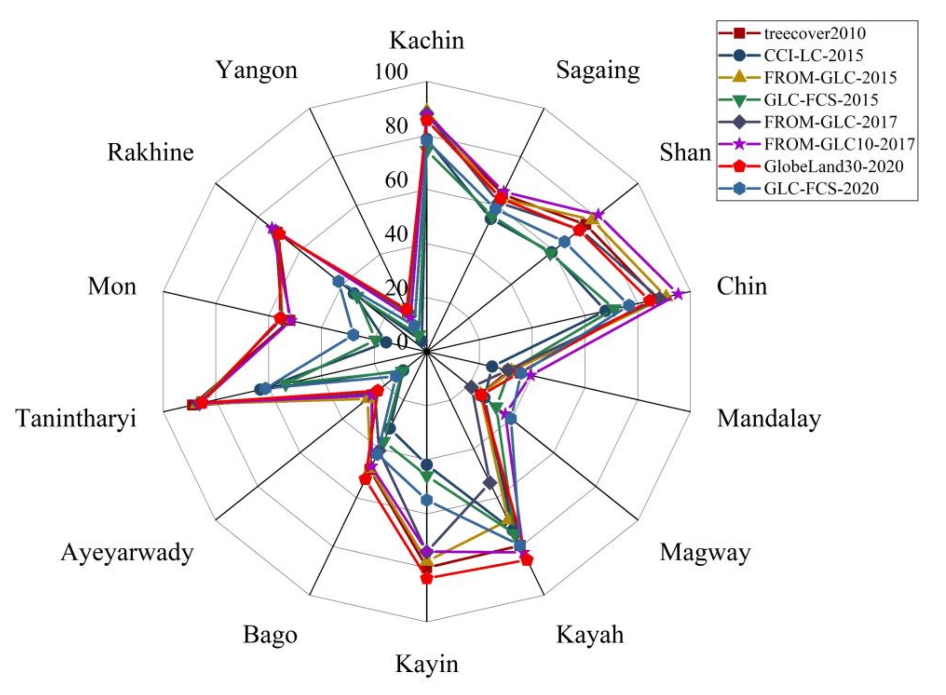
3.2. Comparison of Forest Area

We discussed the differences between these datasets by analyzing the distribution and proportion of forest areas in 14 states of Myanmar in eight datasets. Figure 4 shows the distribution of forest area for all forest datasets.
Overall, the eight datasets have a variable distribution of forest areas in Myanmar. The CCI-LC has the least forest area and FROM-GLC10 has the most forest area. Among the three datasets in 2015, the differences in forest area between CCI-LC and GLC-FCS are small, while the forest area of FROM-GLC exceeds the other two datasets by about 100,000 km2. Since they are from the same year, the effect on the change in forest area due to the expansion or reduction of the actual forest area is small. The reason for such a large difference is mainly related to the objective conditions, such as different remote sensing data sources, classification systems, and production methods. The two datasets of 2017 are essentially the same product FROM-GLC. The difference in forest areas is about 40,000 km2 as seen in Figure 4, and is mainly due to different spatial resolutions. The FROM-GLC10 not only has higher mapping accuracy but also has clearer spatial details, more forests can be identified. The difference in forest area between the two datasets in 2020 is about 60,000 km2.
We further computed the forest proportion in 14 states of Myanmar in eight datasets. As shown in Figure 5, Kayin, Tanintharyi, Mon, and Rakhine have a larger variation in the proportion of different forest datasets. For example, the difference between the maximum and minimum percentages of forest area amounts to 40.34% in Rakhine. There is a difference of 37.11% between the three datasets of the same year in 2015, and 28.03% in the two datasets in 2020. In contrast, the difference between the two same products in 2017 is significantly reduced to 1.79%. However, despite the two datasets for 2017 being essentially the same product, there are cases where there is a large difference in the proportion of forests between states, such as Magway and Kayah. The difference in the proportion of forests between the two datasets is 16.05% for Magway and 28.69% for Kayah. Nevertheless, the overall situation is significantly better than different source datasets, and such large differences are only found in a few states.
Through the comparison of forest areas, it can be seen that the forest cover in Kachin, Sagaing, Mandalay, Yangon is more similar in different datasets. Kachin and the northern areas of Sagaing are higher in altitude, the landscape pattern is mostly plateau, the mountainous forest features can be better identified [38]. Mandalay, Yangon and southern Sagaing are located on plains. These regions are low and flat and dominated by croplands. Forests are better identified when the surrounding land type is mostly cropland [38].

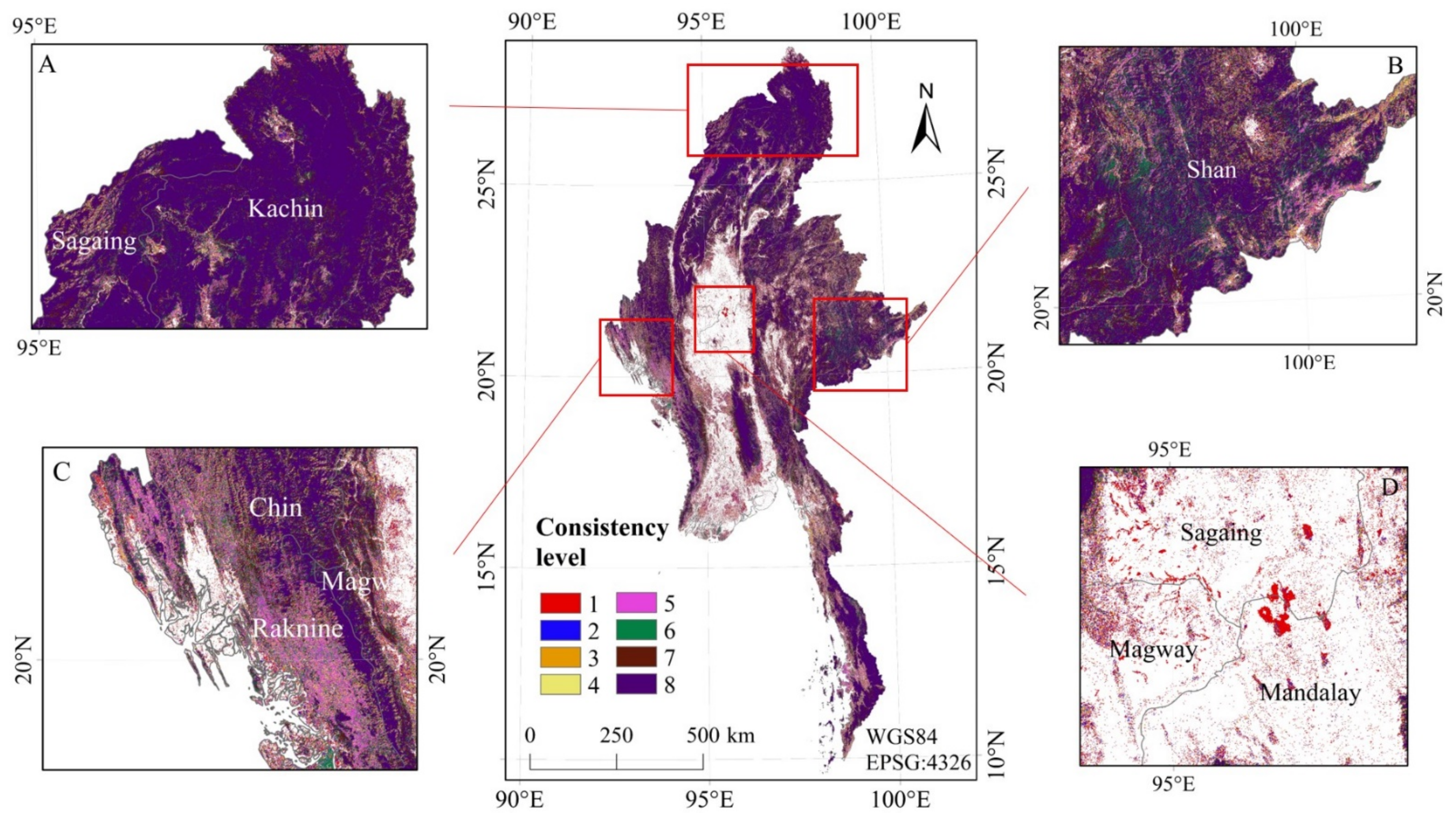
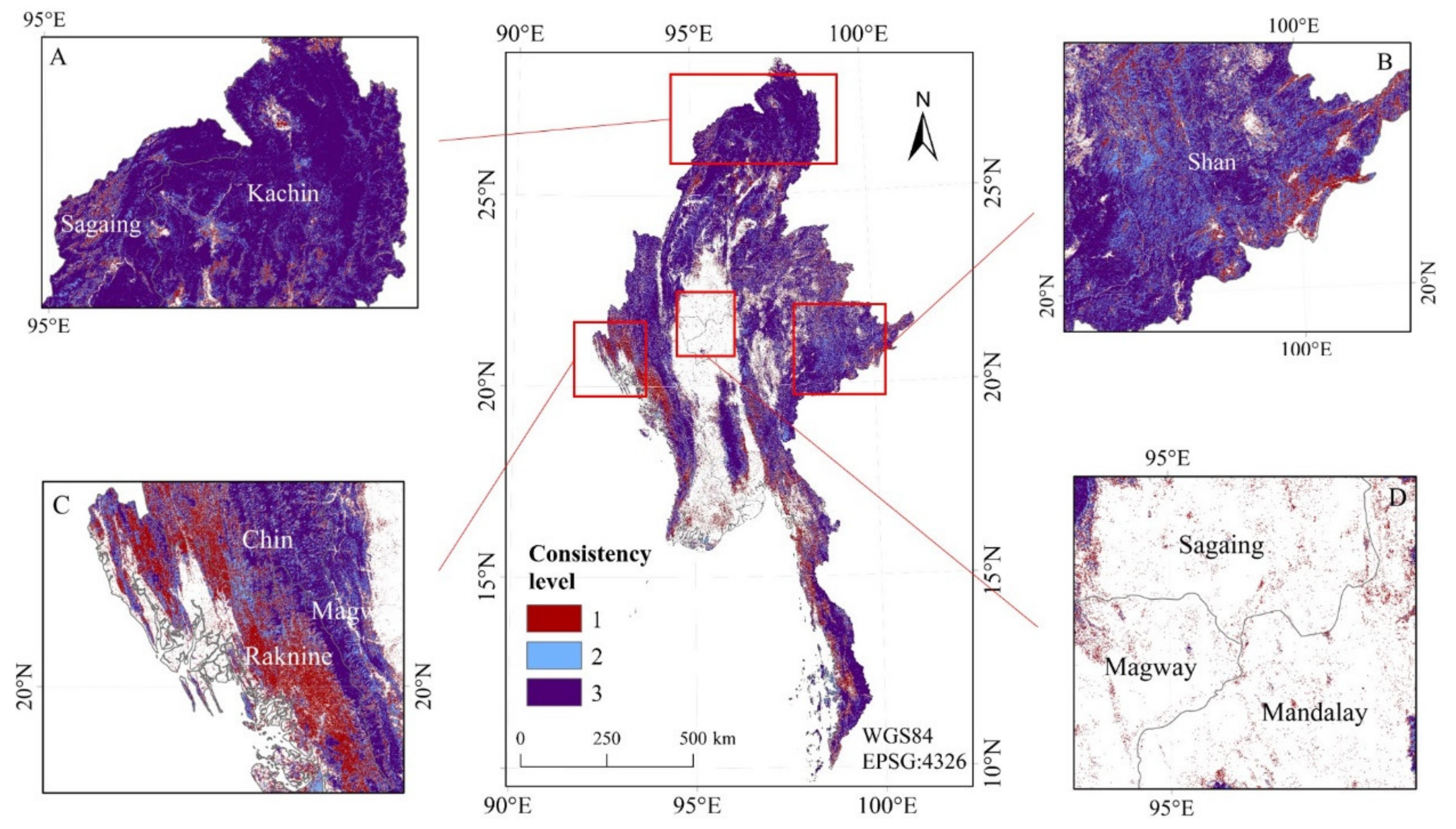
3.3. Spatial Consistency Comparison

3.3.1. Spatial Consistency of Eight Datasets over Different Years

Figure 6 is the spatial consistency map among eight datasets. It can be seen that the consistency of forest distribution in Myanmar is generally good. Sub-areas A and B are regions with a better distribution of forest consistency. The best consistency is found in northern Kachin and northwestern Sagaing (Sub-area A): Northern Myanmar is a highly mountainous region. These areas have high topography, concentrated forest distribution, better continuity, and a relatively homogeneous geographic landscape, so each dataset can identify forests more accurately. Forest consistency is also better in southeastern Shan (Sub-area B), but there are still gaps compared to area A: This is related to the year of the datasets, where deforestation or reforestation affects the temporal distribution of forests. It is also related to the undulating topography of Shan. As for sub-areas C and D, the distribution of forest consistency is less desirable. The spatial distribution of forests in Rakhine and is less consistent (Sub-area C): They are located in southwestern Myanmar with a complex landscape. They are also hotspots of deforestation [39], so the consistency is lower. Mandalay, Magway, and Southern Sagaing are located in the central part of Myanmar (Sub-area D): These regions are flat and dominated by agriculture, the cover type is mostly cropland. Most datasets can classify the land as non-forest. However, occasionally a few datasets are misclassified, resulting in the “salt and pepper” phenomenon.

3.3.2. Spatial Consistency of Three Datasets in 2015

Having fixed the time variables, the forest consistency distribution for the three datasets in 2015 is shown in Figure 7. The sub-areas A-D, respectively, correspond to the sub-areas for the eight datasets. It can be seen that most regions can be guaranteed to have two or more datasets with consistent distributions (Sub-area A and B). Similar to the consistency results for the eight datasets, Rakhine is less consistent, with more areas having a consistency level of 1 (Sub-area C). This is both related to its geographical location and different data sources, classification methods, etc. The “salt and pepper” phenomenon in central Myanmar is less pronounced than in the eight datasets (Sub-area D). The comparison of the three datasets in 2015 removes the effect of time variables, the divergence is mainly related to objective factors in the different datasets.

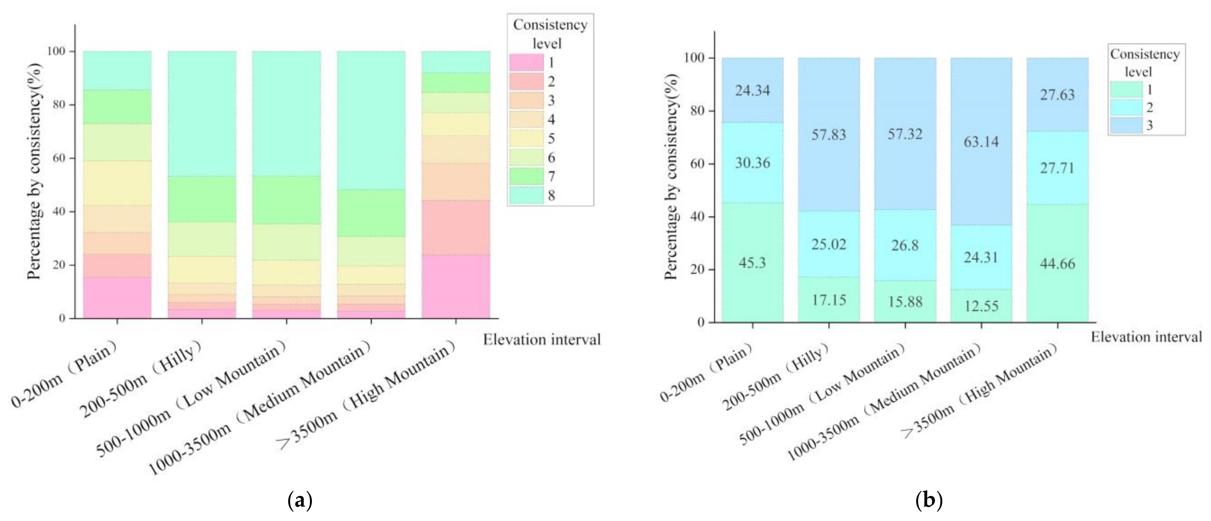
3.4. Factors Influencing on the Spatial Consistency

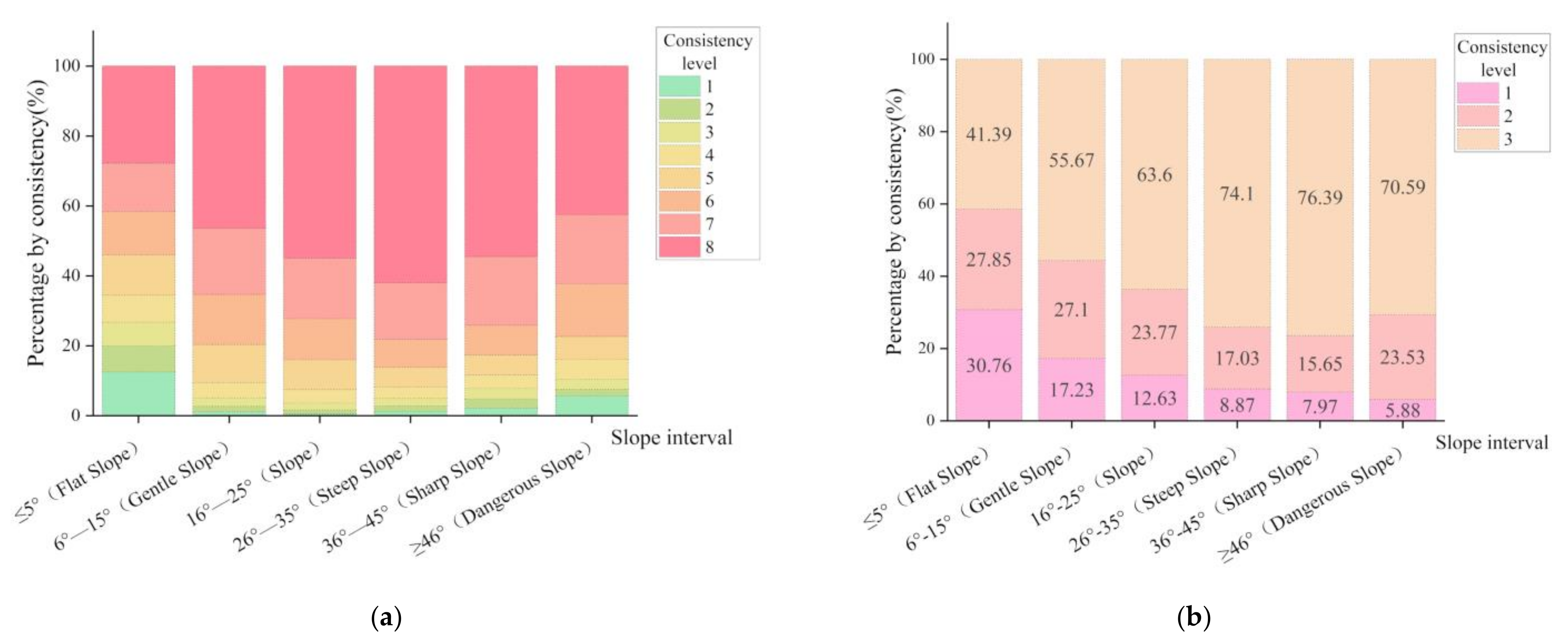
3.4.1. Influence of Terrain on the Consistency

The changes in spatial distribution consistency under different elevations were computed, as shown in Figure 8. In Figure 8a, the proportion of complete consistency is lower in the plain area. While in high mountain areas, the proportion of forests per class decreases with increasing consistency in class. In the regions with hilly, low mountain, and medium mountain (i.e., in the elevation range of 200–3500 m), the proportion of complete consistency in eight datasets is higher. Especially in the medium mountain region, the proportion of complete consistency among datasets exceeds 50%. It indicates that the forests can be identified more accurately from various datasets in these regions. Moreover, the mountains are the main plantation area of forests, the area is vast. It facilitates the interpretation and classification of forests for each dataset. In the areas of plains, the lower consistency among products may be influenced by the confusion of forests with shrubs or cultivated land planted with fruit trees. In the case of high mountain areas, forest extraction is also difficult due to fragmented terrain and fewer planted trees. The distribution pattern of consistency distribution with elevation in the three datasets in 2015 is similar to that of the eight datasets (as shown in Figure 8b). The proportion of complete consistency is also higher in hills, low mountains, and middle mountains.
Figure 9 illustrates the variation of the spatial distribution consistency under different slopes. As shown in Figure 9a, it can be seen that the eight datasets have the highest proportion of complete agreement in each slope interval. As the slope rises, the proportion of complete consistency among datasets shows a trend of increasing and then decreasing. The highest proportion of complete consistency is 62% in the steep slope (26°–35°) interval. The percentage of complete consistency in both slope and sharp slope areas is also over 50%. Except for the flat slope areas, the proportion of forest consistency classes 1–4 in the other slope intervals is very low, which does not exceed 10% or even 5%. It is reasonable to assume that as the slope increases, the geographic landscape is more homogeneous and the forest can be better identified across the datasets. Thus, their consistency results are better. The proportion of complete agreement for each slope interval is greatly increased due to the fixed year variable and the reduction in the number of datasets (Figure 9b). The steep slope and sharp slope interval data sets, respectively, have the best consistency, i.e., 26°–45°, with 74% and 76% complete agreement.

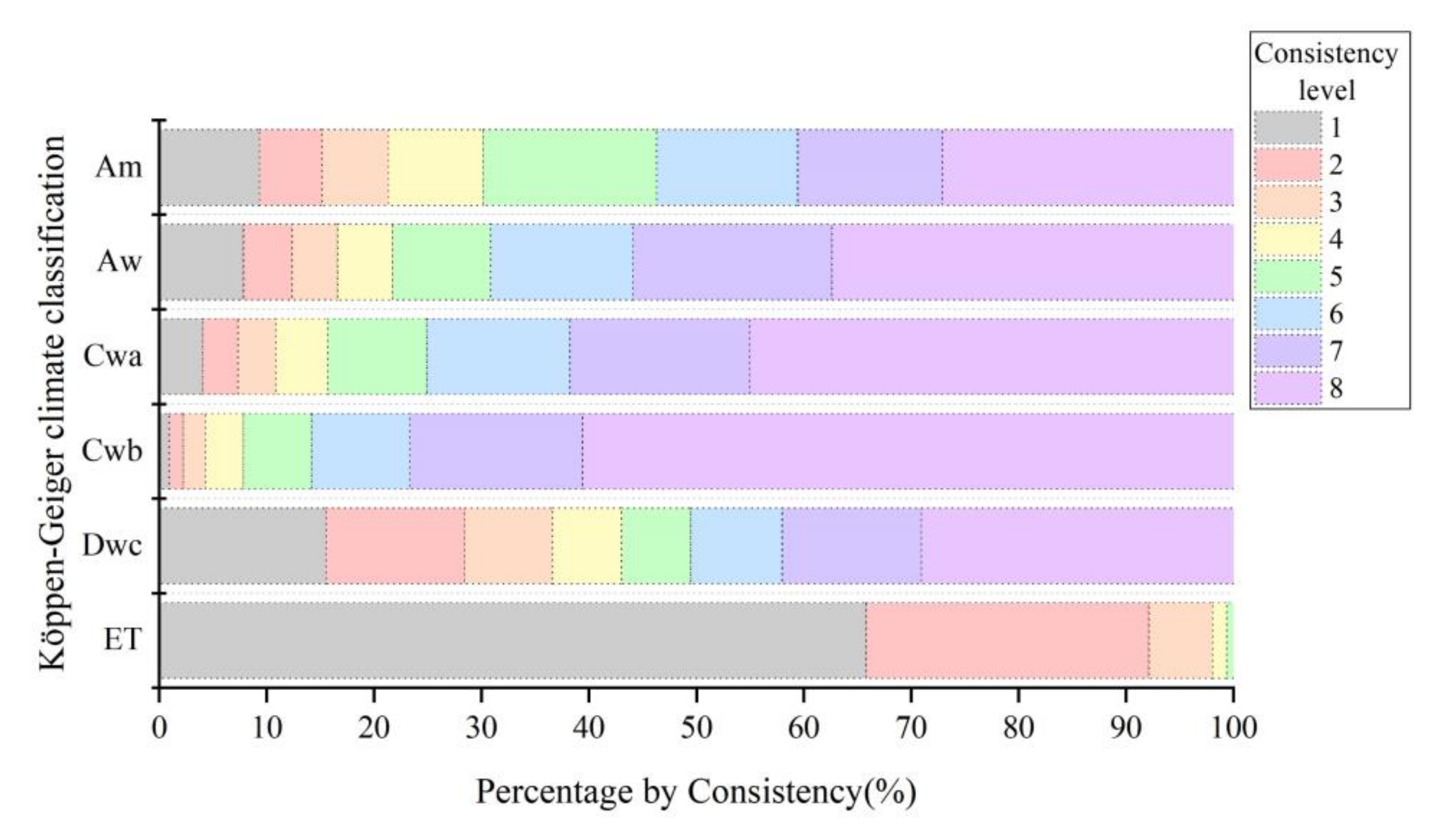
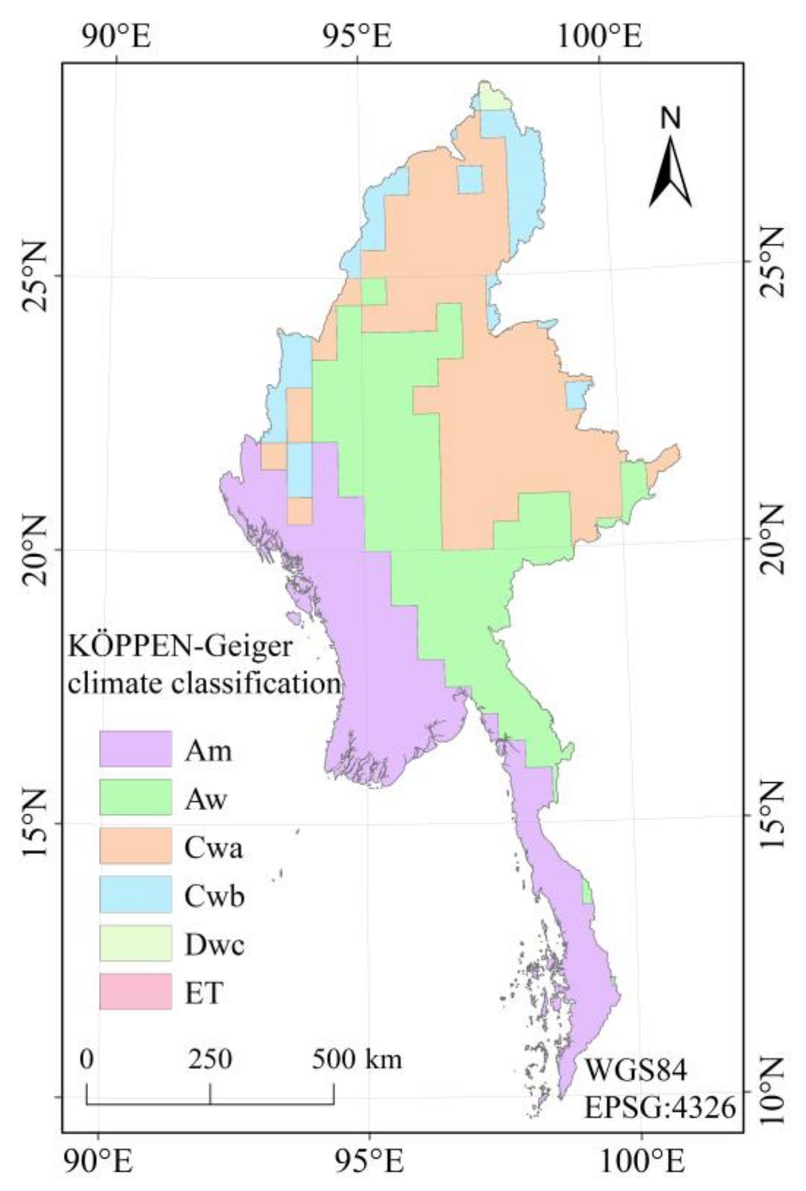
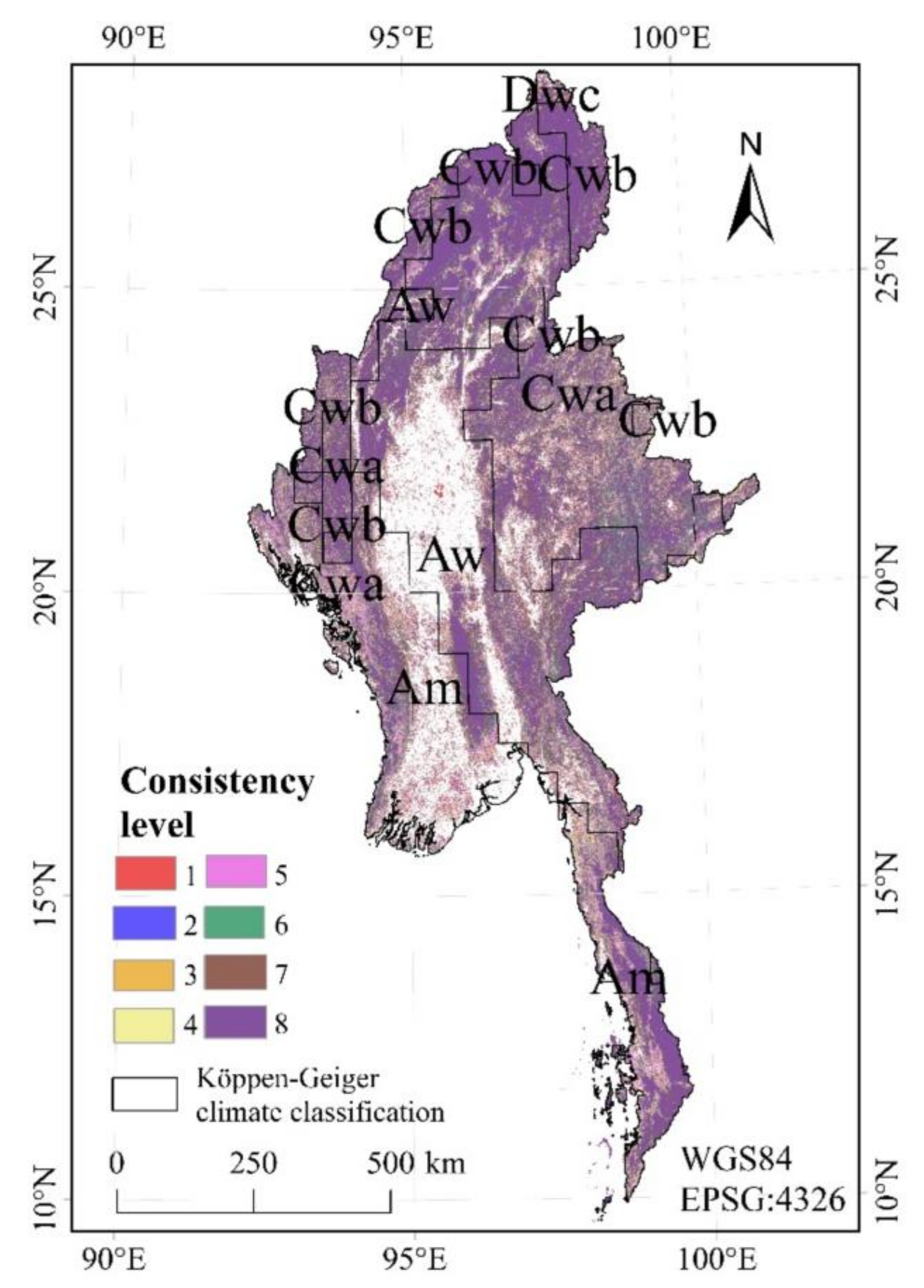
3.4.2. Influence of Climate on the Consistency

To analyze its influence on the consistency of forest datasets, the Köppen–Geiger climate zones were overlapped with the spatial agreement map of the datasets, as shown in Figure 10. The statistics of spatial agreement in each climate zone were further calculated. As elaborated in Figure 11, the highest percentage of complete agreements is mainly in the Cwb and Cwa zone with 60.62% and 45.03%. These two climates are characterized by a yearly suitable temperature and annual precipitation that is not less than the dry value index. Cwb is mainly distributed in high-altitude areas at low and middle latitudes. The objective conditions of combined climate and terrain are suitable for the growth of forests. The dense distribution and large areas of forests make it easier for forest monitoring with different sources of satellite data. The consistency distribution of Aw and Am climatic zones, respectively, followed with 37.41% and 27.11% of complete agreement. Both have monthly average temperatures of 18 °C and above throughout the year, with specific differences in precipitation: Annual precipitation is higher in Am than in Aw, yet the degree of forest complete agreement is higher in Aw. This is because Am is mainly distributed in southwestern Myanmar, including Rakhine, Ayeyarwady, Yangon, and Mon. It is near the sea and the landscape is complex and diverse, forests are easily confused by shrubs and vegetation. While Aw is more distributed in central Myanmar, its feature types are more homogeneous. It is possible to identify forests uniformly from different source datasets. The Dwc and ET climatic zones are less distributed in Myanmar. They both have mostly low temperatures throughout the year, and even ET areas have no precipitation indicators. This makes them unsuitable for forest growth, so their consistency ratios are naturally much lower than those of other climate types.

4. Discussion

4.1. Discrepancies among Datasets

Our study also screened regions with levels 1–4 in the forest consistency map, compared to sample points in the corresponding regions to investigate the misclassification of forests in each dataset.
Figure 12 shows the correct classification of forests and specific misclassification forms for 2015, 2017, and 2020, respectively. The agreement rate between classification and sample points for all three datasets in 2015 is higher than 50%, and the highest correct rate is FROM-GLC at 62.26%. Among the misclassification cases of forests, FROM-GLC mainly misclassified non-forest as forest, while CCI-LC and GLC-FCS more often misclassified forest as non-forest, their percentages are both higher than 30%. In a comprehensive analysis based on the year, the proportion of correctly classified datasets in 2015 is 58.28%. The proportion of forest misclassified as non-forest is 25.58%, which is higher than the proportion of non-forest misclassified as forest at 16.14%. In 2017, the difference is generally lower than in 2015 and 2020 because these two datasets are essentially homogeneous. FROM-GLC has a slightly higher percentage of the misclassified forest as non-forest at 18.24%. FROM-GLC10, on the other hand, has a slightly higher percentage of misclassified non-forest as forest at 23.90%. In 2020, GlobeLand30 has a correct classification of 66.67%, which is also the highest in all datasets. In contrast, GLC-FCS has a lower percentage of correct classifications, and both misclassifications are higher than GlobeLand30, where the misclassification of forest as non-forest is as high as 34.59%.
Several reasons account for the discrepancies among different forest datasets. Firstly, different datasets have their classification schemes [40,41], directly leading to discrepancies. For example, in the classification of low trees, some datasets consider them as forest, as in the case of FROM-GLC, which overestimates its forest area. While some products classify them as shrubs, as in the CCI-LC and GLC-FCS datasets, the forest area is slightly underestimated. There is also a complex definition of “Transitional Woodland” [42]. There is a wide divergence in the interpretation of land types in transition areas across datasets, which may lead to confusion between forest and other vegetation types.
Secondly, different datasets use different satellite images, produced in different ways, and with different spatial resolutions, which will inevitably lead to discrepancies. Furthermore, due to the difference in topography, the spectral response of similar features on the sunny side and the backside of the mountainous area differs greatly. Furthermore, different types of features may reflect similar spectral characteristics, resulting in the phenomenon of “different spectra for the same thing and different things for the same spectra”. In forest mapping, the same tree species may show different spectral reflectance phenomena, presenting different colors and tones in the image. Different tree (shrubs/other vegetation, etc.) species may have similar spectral reflectance properties; they show almost the same color and hue in the image, resulting in interpretation difficulties and leading to confusion or misclassification of forests.
Thirdly, it was found that both terrain and climate can affect the distribution of forests. Most of Myanmar is dominated by a tropical climate, including tropical monsoon climate and savanna climate. The climate is above 18 °C per month throughout the year and precipitation is abundant, providing strong natural conditions for forest growth. Thus, the degree of forest consistency across datasets is relatively better. However, the tropical climate is more prevalent in central and southern Myanmar. The terrain is flatter, human activities are complex, the total amount of forest is reduced, and the landscape type is dominated by cropland and constructed land. In contrast, although northern Myanmar has a predominantly subtropical climate, temperatures and precipitation conditions slightly less favorable than those of the tropics. However, its high terrain allows for less human interference and dense, continuous forest growth. The high altitude also limits deforestation, so northern Myanmar has the best forest consistency.
The actual forest changes due to the year’s changes cannot be ignored. Figure 13 specifically depicts the differences between datasets due to actual forest changes.

4.2. Challenges and Prospect of Forest Mapping at Large Scale

Through the comparative analysis of forests in Myanmar, we found that a challenge in forest mapping at large scales was the spatial resolution and classification methods. The current land cover dataset is still dominated by low to medium resolution and with automatic classification methods, which impose limitations on the mapping of forests. From the results of the accuracy assessment in this paper, the forest mapping accuracy of FROM-GLC10 with 10 m resolution is the highest, but the best forest classification of GlobeLand30 is obtained by combining various accuracy indicators. Firstly, the higher spatial resolution of GlobeLand30 plays an important role in high precision mapping. Multiple imaging sources from satellites such as Landsat 8, sentinel, and GF, as well as the development of machine learning, also provide sufficient guarantees for high spatial resolution mapping [43,44]. Secondly, GlobeLand30 adopts the POK classification method, while adding manual checking and knowledge modification based on automatic computer classification. It can achieve better accuracy results, although the mapping efficiency is reduced. Mixed image elements also affect forest mapping. Even the FROM-GLC10 inevitably has mixed pixels, but improving the spatial resolution can alleviate the problem to some extent. In terms of the solution method, a decision tree combined with mixed image element decomposition can be used [45]. A percentage soft classification scheme can also be used instead of the traditional binary classification, the ratio can reflect the distribution of forest within a pixel [25]. They can also effectively solve the problem of mixed image elements.
NDVI, EVI, and reflectance data are still the three main types of satellite data for forest mapping, making full use of the implied phenological information in NDVI and EVI is important [46]. In the development of remote sensing mapping, it has been shown that adding other data sources such as radar data, hyperspectral data, and so on, can provide new possibilities for surface coverage mapping [47,48,49,50].
Nowadays, remote sensing mapping and applications are developing rapidly. Data sources are becoming more abundant and progressively more accurate. The WFV (Wide Field of View) image of GF-6 has two new red-edge bands compared with the similar image of GF-1, which is helpful to improve the monitoring capability of the forest [51]. The methods of land cover monitoring have also evolved with the times. Tsinghua University has proposed the conceptual framework of smart remote sensing mapping. They led to the completion of the 30 m resolution global day-by-day satellite remote sensing data cube (SDC), and the seasonal global surface coverage map over 36 years [52]. It helps to significantly advance the development of remote sensing applications, provides decision support for land resource management, and contributes greatly to future forest monitoring and mapping. In addition, the development of cloud computing also supplies an effective means for remote sensing forest monitoring. For example, Google Earth Engine (GEE) provides a global-scale geospatial analysis service [53] that can be used to monitor global forest changes.

5. Conclusions

This study presented a comparative analysis and comprehensive evaluation of forest cover from widely-used land cover datasets in Myanmar: Sufficient forest samples over 4 years were randomly collected from GE, which are used to conduct an accurate and objective evaluation of each dataset. The similarities and differences in the spatial distribution were compared for these forest datasets. The influence on spatial consistency was further analyzed from the aspects of terrain and climatic conditions.
The results indicate that GlobeLand30 has the best comprehensive accuracy in Myanmar, followed by the FROM-GLC series, Hansen Forest cover, and the last is the CCI-LC and GLC-FCS series. The consistent forest distribution of these datasets is best in northern Myanmar. There, the terrain is relatively high, forest distribution is continuous, and the feature types are relatively homogeneous, so the remote sensing images have a certain degree of differentiation. The mapping results are quite good, even for the data with low spatial resolution. In contrast, the southwestern region of Myanmar is at a lower altitude and near the sea, the landscape is more complex, the mixing of forests, shrubs, and cropland is serious. This will be the key direction for future efforts in forest mapping. In addition, this study also analyzed the limiting factors (terrain and climate) affecting forest consistency. We found that the areas with the best consistency are, respectively, distributed in the range of 1000–3500 m in elevation and 26°–35° in slope, and the subtropical highland climate (Cwb) zone. Although the tropical climate is more favorable for forest growth, it is mostly distributed in lower terrain areas with fewer forests and high human activity. The higher terrain of northern Myanmar, with its Cwb climate, is more conducive to forest growth than a tropical climate.
Nowadays, all countries in the world are facing a critical situation of forest degradation, especially in tropical countries. Comparing multiple datasets can help users to select the appropriate data in different regions to conduct research. It can provide policy recommendations in line with local forest planning. As for Myanmar, forest monitoring is still a challenging task, with data sources, landscapes, and classification methods being the main constraints to its accuracy [38,54,55]. In the future, forest monitoring can be improved with multi-source remote sensed data and deep learning approaches.

Author Contributions

Conceptualization, H.X.; Data curation, D.H.; Formal analysis, H.X.; Methodology, H.X., J.N. and D.H.; Software, J.N., C.L. (Chang Liu), B.C. and L.Z.; Validation, J.N., S.Y., W.H. and C.L. (Cansong Li); Writing—original draft, H.X. and J.N.; Writing—review and editing, C.L. (Chang Liu), B.C., S.Y., D.H., L.Z., W.H. and C.L. (Cansong Li). All authors have read and agreed to the published version of the manuscript.

Funding

This research was funded by the National Natural Science Foundation of China (41801308); Reserve Talent Program for Young and Middle-aged Academic and Technical Leaders in Yunnan Province (202105AC160059); Key Laboratory of Land Satellite Remote Sensing Application Center, Ministry of Natural Resources of the People’s Republic of China (KLSMNR-202105); Open Fund of State Laboratory of Information Engineering in Surveying, Mapping and Remote Sensing, Wuhan University (No.20S01); Doctoral Research Fund of Shandong Jianzhu University (XNBS1804); and Yunnan Fundamental Research Projects (202001AS070032).

Institutional Review Board Statement

Not applicable.

Informed Consent Statement

Not applicable.

Data Availability Statement

Not applicable.

Conflicts of Interest

The authors declare no conflict of interest.

References

  1. Sullivan, B.W.; Nifong, R.L.; Nasto, M.K.; Alvarez-Clare, S.; Dencker, C.M.; Soper, F.M.; Shoemaker, K.T.; Ishida, F.Y.; Zaragoza-Castells, J.; Davidson, E.A. Biogeochemical recuperation of lowland tropical forest during succession. Ecology 2019, 100, e02641. [Google Scholar] [CrossRef] [PubMed] [Green Version]
  2. Hill, S.L.L.; Arnell, A.; Maney, C.; Butchart, S.H.M.; Hilton-Taylor, C.; Ciciarelli, C.; Davis, C.; Dinerstein, E.; Purvis, A.; Burgess, N.D. Measuring Forest Biodiversity Status and Changes Globally. Front. For. Glob. Chang. 2019, 2, 70. [Google Scholar] [CrossRef]
  3. Laurin, G.V.; Vittucci, C.; Tramontana, G.; Ferrazzoli, P.; Guerriero, L.; Papale, D. Monitoring tropical forests under a functional perspective with satellite-based vegetation optical depth. Glob. Chang. Biol. 2020, 26, 3402–3416. [Google Scholar] [CrossRef] [PubMed]
  4. Lwin, K.K.; Ota, T.; Shimizu, K.; Mizoue, N. A country-scale analysis revealed effective land-use zoning affecting forest cover changes in Myanmar. J. For. Res. 2020, 25, 389–396. [Google Scholar] [CrossRef]
  5. Lee, D.K. Challenging forestry issues in Asia and their strategies. RAP Publ. 2009, 3, 65–76. [Google Scholar]
  6. Aye, W.N.; Wen, Y.; Marin, K.; Thapa, S.; Tun, A.W. Contribution of Mangrove Forest to the Livelihood of Local Communities in Ayeyarwaddy Region, Myanmar. Forests 2019, 10, 414. [Google Scholar] [CrossRef] [Green Version]
  7. Htun, N.Z.; Mizoue, N.; Kajisa, T.; Yoshida, S. Deforestation and forest degradation as measures of Popa Mountain Park (Myanmar) effectiveness. Environ. Conserv. 2009, 36, 218–224. [Google Scholar] [CrossRef]
  8. Lechner, A.M.; Foody, G.M.; Boyd, D.S. Applications in Remote Sensing to Forest Ecology and Management. One Earth 2020, 2, 405–412. [Google Scholar] [CrossRef]
  9. Gao, Y.; Skutsch, M.; Paneque-Gálvez, J.; Ghilardi, A. Remote sensing of forest degradation: A review. Environ. Res. Lett. 2020, 15, 103001. [Google Scholar] [CrossRef]
  10. Pettorelli, N.; Bühne, H.S.T.; Tulloch, A.; Dubois, G.; Macinnis-Ng, C.; Queirós, A.M.; Keith, D.A.; Wegmann, M.; Schrodt, F.; Stellmes, M.; et al. Satellite remote sensing of ecosystem functions: Opportunities, challenges and way forward. Remote Sens. Ecol. Conserv. 2017, 4, 71–93. [Google Scholar] [CrossRef]
  11. Hansen, M.C.; Reed, B.W. A comparison of the IGBP DISCover and University of Maryland 1 km global land cover products. Int. J. Remote Sens. 2000, 21, 1365–1373. [Google Scholar] [CrossRef]
  12. Loveland, T.R.; Belward, A.S. The IGBP-DIS global 1km land cover data set, DISCover: First results. Int. J. Remote Sens. 1997, 18, 3289–3295. [Google Scholar] [CrossRef]
  13. Loveland, T.R.; Reed, B.C.; Brown, J.; Ohlen, D.; Zhu, Z.; Yang, L.; Merchant, J.W. Development of a global land cover characteristics database and IGBP DISCover from 1 km AVHRR data. Int. J. Remote Sens. 2000, 21, 1303–1330. [Google Scholar] [CrossRef]
  14. Bartholomé, E.; Belward, A.S. GLC2000: A new approach to global land cover mapping from Earth observation data. Int. J. Remote Sens. 2005, 26, 1959–1977. [Google Scholar] [CrossRef]
  15. Friedl, M.A.; McIver, D.K.; Baccini, A.; Gao, F.; Schaaf, C.; Hodges, J.C.F.; Zhang, X.Y.; Muchoney, D.; Strahler, A.H.; Woodcock, C.E.; et al. Global land cover mapping from MODIS: Algorithms and early results. Remote Sens Environ. 2002, 83, 287–302. [Google Scholar] [CrossRef]
  16. Friedl, M.A.; Sulla-Menashe, D.; Tan, B.; Schneider, A.; Ramankutty, N.; Sibley, A.; Huang, X. MODIS Collection 5 global land cover: Algorithm refinements and characterization of new datasets. Remote Sens. Environ. 2010, 114, 168–182. [Google Scholar] [CrossRef]
  17. Arino, O.; Bicheron, P.; Achard, F.; Latham, J.; Witt, R.; Weber, J.-L. The most detailed portrait of Earth. Eur. Sp. Agency 2008, 136, 25–31. [Google Scholar]
  18. Bontemps, S.; Defourny, P.; van Bogaert, E.; Kalogirou, V.; Perez, J.R. GLOBCOVER 2009 Products Description and Validation Report. ESA Bull. 2011, 136, 53. [Google Scholar]
  19. Defourny, P.; Kirches, G.; Brockmann, C.; Boettcher, M.; Peters, M.; Bontemps, S.; Lamarche, C.; Schlerf, M.; Santoro, M. Product User Guide Version; ESA Climate Office: Harwell, UK, 2012; Volume 2, p. 325. [Google Scholar]
  20. Gong, P.; Wang, J.; Yu, L.; Zhao, Y.; Zhao, Y.; Liang, L.; Niu, Z.; Huang, X.; Fu, H.; Liu, S.; et al. Finer resolution observation and monitoring of global land cover: First mapping results with Landsat TM and ETM+ data. Int. J. Remote Sens. 2012, 34, 2607–2654. [Google Scholar] [CrossRef] [Green Version]
  21. Yu, L.; Wang, J.; Gong, P. Improving 30 m global land-cover map FROM-GLC with time series MODIS and auxiliary data sets: A segmentation-based approach. Int. J. Remote Sens. 2013, 34, 5851–5867. [Google Scholar] [CrossRef]
  22. Chen, J.; Chen, J.; Liao, A.; Cao, X.; Chen, L.; Chen, X.; He, C.; Han, G.; Peng, S.; Lu, M.; et al. Global land cover mapping at 30 m resolution: A POK-based operational approach. ISPRS J. Photogramm. Remote Sens. 2015, 103, 7–27. [Google Scholar] [CrossRef] [Green Version]
  23. Gong, P.; Liu, H.; Zhang, M.; Li, C.; Wang, J.; Huang, H.; Clinton, N.; Ji, L.; Li, W.; Bai, Y.; et al. Stable classification with limited sample: Transferring a 30-m resolution sample set collected in 2015 to mapping 10-m resolution global land cover in 2017. Sci. Bull. 2019, 64, 370–373. [Google Scholar] [CrossRef] [Green Version]
  24. Gao, Y.; Liu, L.; Zhang, X.; Chen, X.; Mi, J.; Xie, S. Consistency Analysis and Accuracy Assessment of Three Global 30-m Land-Cover Products over the European Union using the LUCAS Dataset. Remote Sens. 2020, 12, 3479. [Google Scholar] [CrossRef]
  25. Wei, Y.; Lu, M.; Wu, W.; Ru, Y. Multiple factors influence the consistency of cropland datasets in Africa. Int. J. Appl. Earth Obs. Geoinf. 2020, 89, 102087. [Google Scholar] [CrossRef]
  26. Pérez-Hoyos, A.; Rembold, F.; Kerdiles, H.; Gallego, J. Comparison of Global Land Cover Datasets for Cropland Monitoring. Remote Sens. 2017, 9, 1118. [Google Scholar] [CrossRef] [Green Version]
  27. Hansen, M.C.; Potapov, P.V.; Moore, R.; Hancher, M.; Turubanova, S.A.; Tyukavina, A.; Thau, D.; Stehman, S.V.; Goetz, S.J.; Loveland, T.R. High-resolution global maps of 21st-century forest cover change. Science 2013, 342, 850–853. [Google Scholar] [CrossRef] [Green Version]
  28. Hui, Z.; Fu, X.; Jinwei, D. Research ON Forest Resource Changes Monitoring Based ON Multi-Source Remote Sensing Images—Taking the Loess Plateau as an Example; Beijing Forestry University: Beijing, China, 2020. [Google Scholar]
  29. Zhang, X.; Liu, L.; Chen, X.; Xie, S.; Gao, Y. Fine Land-Cover Mapping in China Using Landsat Datacube and an Operational SPECLib-Based Approach. Remote Sens. 2019, 11, 1056. [Google Scholar] [CrossRef] [Green Version]
  30. Zhang, X.; Liu, L.; Chen, X.; Gao, Y.; Xie, S.; Mi, J. GLC_FCS30: Global land-cover product with fine classification system at 30 m using time-series Landsat imagery. Earth Syst. Sci. Data 2021, 13, 2753–2776. [Google Scholar] [CrossRef]
  31. Zhao, Y.; Gong, P.; Yu, L.; Hu, L.; Li, X.; Li, C.; Zhang, H.; Zheng, Y.; Wang, J.; Zhao, Y.; et al. Towards a common validation sample set for global land-cover mapping. Int. J. Remote Sens. 2014, 35, 4795–4814. [Google Scholar] [CrossRef]
  32. Farr, T.; Kobrick, M. Shuttle radar topography mission produces a wealth of data. Eos Trans. Am. Geophys. Union 2000, 81, 583–585. [Google Scholar] [CrossRef]
  33. Rabus, B.; Eineder, M.; Roth, A.; Bamler, R. The shuttle radar topography mission—A new class of digital elevation models acquired by spaceborne radar. ISPRS J. Photogramm. Remote Sens. 2003, 57, 241–262. [Google Scholar] [CrossRef]
  34. Rubel, F.; Kottek, M. Observed and projected climate shifts 1901-2100 depicted by world maps of the Köppen-Geiger climate classification. Meteorol. Z. 2010, 19, 135–141. [Google Scholar] [CrossRef] [Green Version]
  35. Chen, D.; Lu, M.; Zhou, Q.; Xiao, J.; Ru, Y.; Wei, Y.; Wu, W. Comparison of Two Synergy Approaches for Hybrid Cropland Mapping. Remote Sens. 2019, 11, 213. [Google Scholar] [CrossRef] [Green Version]
  36. Kang, J.; Wang, Z.; Sui, L.; Yang, X.; Ma, Y.; Wang, J. Consistency Analysis of Remote Sensing Land Cover Products in the Tropical Rainforest Climate Region: A Case Study of Indonesia. Remote Sens. 2020, 12, 1410. [Google Scholar] [CrossRef]
  37. Xu, Y.; Yu, L.; Feng, D.; Peng, D.; Li, C.; Huang, X.; Lu, H.; Gong, P. Comparisons of three recent moderate resolution African land cover datasets: CGLS-LC100, ESA-S2-LC20, and FROM-GLC-Africa30. Int. J. Remote Sens. 2019, 40, 6185–6202. [Google Scholar] [CrossRef]
  38. Yang, R.; Luo, Y.; Yang, K.; Hong, L.; Zhou, X. Analysis of Forest Deforestation and its Driving Factors in Myanmar from 1988 to 2017. Sustainability 2019, 11, 3047. [Google Scholar] [CrossRef] [Green Version]
  39. Wang, C.; Myint, S.W. Environmental Concerns of Deforestation in Myanmar 2001–2010. Remote Sens. 2016, 8, 728. [Google Scholar] [CrossRef] [Green Version]
  40. Nabil, M.; Zhang, M.; Bofana, J.; Wu, B.; Stein, A.; Dong, T.; Zeng, H.; Shang, J. Assessing factors impacting the spatial discrepancy of remote sensing based cropland products: A case study in Africa. Int. J. Appl. Earth Obs. Geoinf. 2020, 85, 102010. [Google Scholar] [CrossRef]
  41. Arjasakusuma, S.; Pribadi, U.A.; Seta, G.A. Accuracy and Spatial Pattern Assessment of Forest Cover Change Datasets in Central Kalimantan. Indones. J. Geogr. 2018, 50, 222–227. [Google Scholar] [CrossRef]
  42. Manakos, I.; Tomaszewska, M.; Gkinis, I.; Brovkina, O.; Filchev, L.; Genc, L.; Gitas, I.Z.; Halabuk, A.; Inalpulat, M.; Irimescu, A.; et al. Comparison of Global and Continental Land Cover Products for Selected Study Areas in South Central and Eastern European Region. Remote Sens. 2018, 10, 1967. [Google Scholar] [CrossRef] [Green Version]
  43. Feng, D.; Yu, L.; Zhao, Y.; Cheng, Y.; Xu, Y.; Li, C.; Gong, P. A multiple dataset approach for 30-m resolution land cover mapping: A case study of continental Africa. Int. J. Remote Sens. 2018, 39, 3926–3938. [Google Scholar] [CrossRef]
  44. Lesiv, M.; Fritz, S.; McCallum, I.; Tsendbazar, N.; Herold, M.; Pekel, J.-F. Evaluation of ESA CCI prototype land cover map at 20 m. Int. Inst. Appl. Syst. Anal. IIASA 2017. [Google Scholar] [CrossRef]
  45. Cui, L.; Du, H.; Zhou, G.; Li, X.; Mao, F.; Xu, X.; Fan, W.; Li, Y.; Zhu, D.; Liu, T.; et al. Combination of decision tree and mixed pixel decomposition for extracting bamboo forest information in China. Remote Sens. 2019, 23, 166–176. [Google Scholar]
  46. Arekhi, M.; Goksel, C.; Sanli, F.B.; Senel, G. Comparative Evaluation of the Spectral and Spatial Consistency of Sentinel-2 and Landsat-8 OLI Data for Igneada Longos Forest. ISPRS Int. J. Geo-Inf. 2019, 8, 56. [Google Scholar] [CrossRef] [Green Version]
  47. Reiche, J.; Hamunyela, E.; Verbesselt, J.; Hoekman, D.; Herold, M. Improving near-real time deforestation monitoring in tropical dry forests by combining dense Sentinel-1 time series with Landsat and ALOS-2 PALSAR-2. Remote Sens. Environ. 2018, 204, 147–161. [Google Scholar] [CrossRef]
  48. Sui, L.; Kang, J.; Yang, X.; Wang, Z.; Wang, J. Inconsistency distribution patterns of different remote sensing land-cover data from the perspective of ecological zoning. Open Geosci. 2020, 12, 324–341. [Google Scholar] [CrossRef]
  49. Fang, X.; Zhao, W.; Zhang, C.; Zhang, D.; Wei, X.; Qiu, W.; Ye, Y. Methodology for credibility assessment of historical global LUCC datasets. Sci. China Earth Sci. 2020, 63, 1013–1025. [Google Scholar] [CrossRef]
  50. Lossou, E.; Owusu-Prempeh, N.; Agyemang, G. Monitoring Land Cover changes in the tropical high forests using multi-temporal remote sensing and spatial analysis techniques. Remote Sens. Appl. Soc. Environ. 2019, 16, 100264. [Google Scholar] [CrossRef]
  51. Huang, J.; Li, Z.; Chen, E.; Zhao, L.; Bingping, M.O. Classification of plantation types based on WFV multispectral imagery of the GF-6 satellite. Remote Sens. 2021, 25, 539–548. [Google Scholar]
  52. Liu, H.; Gong, P.; Wang, J.; Wang, X.; Ning, G.; Xu, B. Production of global daily seamless data cubes and quantification of global land cover change from 1985 to 2020 iMap World 1.0. Remote Sens. Environ. 2021, 258, 112364. [Google Scholar] [CrossRef]
  53. Zurqani, H.A.; Post, C.J.; Mikhailova, E.A.; Schlautman, M.; Sharp, J.L. Geospatial analysis of land use change in the Savannah River Basin using Google Earth Engine. Int. J. Appl. Earth Obs. Geoinf. 2018, 69, 175–185. [Google Scholar] [CrossRef]
  54. Reddy, C.S.; Pasha, S.V.; Satish, K.; Unnikrishnan, A.; Chavan, S.B.; Jha, C.S.; Diwakar, P.G.; Dadhwal, V.K. Quantifying and predicting multi-decadal forest cover changes in Myanmar: A biodiversity hotspot under threat. Biodivers. Conserv. 2019, 28, 1129–1149. [Google Scholar] [CrossRef]
  55. Leimgruber, P.; Kelly, D.S.; Steininger, M.K.; Brunner, J.; Müller, T.; Songer, M. Forest cover change patterns in Myanmar (Burma) 1990–2000. Environ. Conserv. 2005, 32, 356–364. [Google Scholar] [CrossRef] [Green Version]
Figure 1. Spatial distribution of forest and non-forest validation samples in Myanmar (2020).
Applsci 11 11348 g001
Figure 2. KÖPPEN-Geiger climate zones in Myanmar.
Applsci 11 11348 g002
Figure 3. Spatial distribution of forests in Myanmar extracted from eight global land cover datasets. (a) Hansen2010; (b) CCI-LC-2015; (c) FROM-GLC-2015; (d) GLC-FCS-2015; (e) FROM-GLC-2017; (f) FROM-GLC10; (g) GLC-FCS-2020; (h) GlobeLand30-2020.
Applsci 11 11348 g003
Figure 4. Eight global land cover datasets on forest area in Myanmar (Purple indicates the dataset of year 2010, Orange indicates the dataset of year 2015, Green indicates the dataset of year 2017, Blue indicates the dataset of year 2020).
Applsci 11 11348 g004
Figure 5. Percentage of forest cover by state in different datasets.
Applsci 11 11348 g005
Figure 6. Spatial consistency of eight datasets in Myanmar. Full agreement corresponds to a value of 8 (all eight datasets agree), and full disagreement corresponds to a value of 1 (only one dataset identifies forest). White corresponds to non-forest for all datasets. Sub-area (AD), respectively, are the details of the consistency distribution for four major regions ((A) is the area of the best consistency, (B) is the area of good consistency, (C) is the area of poor consistency, (D) is the area with “salt and pepper”).
Applsci 11 11348 g006
Figure 7. Spatial consistency of three datasets in 2015. Full agreement corresponds to a value of 3 (all three datasets agree), and full disagreement corresponds to a value of 1 (only one dataset identifies forest). White corresponds to no forest for all datasets. Sub-area (AD), respectively, are the details of the consistency distribution for four major regions ((A) is the area of the best consistency, (B) is the area of good consistency, (C) is the area of poor consistency, (D) is the area with “salt and pepper”).
Applsci 11 11348 g007
Figure 8. Consistency distribution among different elevation intervals. (a) Eight datasets; (b) Three datasets in 2015.
Applsci 11 11348 g008
Figure 9. Consistency distribution among different slope intervals. (a) Eight datasets; (b) Three datasets in 2015.
Applsci 11 11348 g009
Figure 10. Spatial consistency of eight datasets with KÖPPEN-Geiger climate classification.
Applsci 11 11348 g010
Figure 11. The proportion of eight spatial consistency levels in 6 climate zones.
Applsci 11 11348 g011
Figure 12. Proportion of forest datasets correctly classified and two incorrectly classified in 2015/2017/2020. (a) Three datasets in 2015; (b) Two datasets in 2017; (c) Two datasets in 2020.
Applsci 11 11348 g012
Figure 13. Examples of actual forest change in Myanmar, 2010–2020. (a) Differences between datasets; (b) Actual forest change during 4 years.
Applsci 11 11348 g013
Table 1. Summary of the main characteristics of global land cover datasets.
DatasetTimeSatelliteSpatial ResolutionClassification
Scheme
Hansen2010Landsat 7 ETM+30 m
CCI-LC2015ENVISAT/MERIS/
SPOT-VGT/PROBA-V
300 mLCCS
FROM-GLC2015Landsat TM/ETM+/OLI30 mTwo level classification system of level 1 and level 2
201730 m10 classes
FROM-GLC10
(2017)
LandsatTM/ETM/OLI/
Sentinel-2
10 m10 classes
GLC-FCS2015Landsat TM/ETM+/OLI30 mGlobal surface
fine classification
2020Landsat/Sentinel-1SAR30 mGlobal surface
fine classification
GlobeLand302020Landsat TM5/ETM+/OLI/
HJ-1/GF-1
30 m10 classes
Table 2. Forest classification systems from the eight datasets and the conversion table.
DatasetTimeForest Related Types and Codes
Hansen
(treecover)
2010Forest
CCI-LC201550: Tree cover, broadleaved, evergreen, closed to open (>15%)
60, 61, 62: Tree cover, broadleaved, deciduous, closed to open (>15%)
70, 71, 72: Tree cover, needleleaved, evergreen, closed to open (>15%)
80, 81, 82: Tree cover, needleleaved, deciduous, closed to open (>15%)
90: Tree cover, mixed leaf type (broadleaved and needleleaved)
100: Mosaic tree and shrub (>50%)/herbaceous cover (<50%)
160: Tree cover, flooded, fresh or brakish water
170: Tree cover, flooded, saline water
FROM-GLC201521: Broadleaf, leaf-on
22: Broadleaf, leaf-off
23: Needleleaf, leaf-on
24: Needleleaf, leaf-off
25: Mixed leaf, leaf-on
26: Mixed leaf, leaf-off
20172: Forest
FROM-GLC10
(2017)
20: Forest
GLC-FCS201550: Evergreen broadleaved forest
60: Deciduous broadleaved forest
61: Open deciduous broadleaved forest (0.15 < fc < 0.4)
62: Closed deciduous broadleaved forest (fc> 0.4)
70: Evergreen needle-leaved forest
71: Open evergreen needle-leaved forest (0.15 < fc < 0.4)
72: Closed evergreen needle-leaved forest (fc > 0.4)
80: Deciduous needle-leaved forest
81: Open deciduous needle-leaved forest (0.15 < fc < 0.4)
82: Closed deciduous needle-leaved forest (fc > 0.4)
90: Mixed leaf forest (broadleaved and needle-leaved)
202051: Open evergreen broadleaved forest
52: Closed evergreen broadleaved forest
61: Open deciduous broadleaved forest (0.15 < fc < 0.4)
62: Closed deciduous broadleaved forest (fc > 0.4)
71: Open evergreen needle-leaved forest (0.15 < fc < 0.4)
72: Closed evergreen needle-leaved forest (fc > 0.4)
81: Open deciduous needle-leaved forest (0.15 < fc < 0.4)
82: Closed deciduous needle-leaved forest (fc > 0.4)
91: Open mixed leaf forest (broadleaved and needle-leaved)
92: Closed mixed leaf forest (broadleaved and needle-leaved)
GlobeLand30202020: Forest (The land covered by trees with crown coverage of more than 30%, including deciduous broad-leaved forest, evergreen broad-leaved forest, deciduous coniferous forest, evergreen coniferous forest, mixed forest, and sparse forest land with crown coverage of 10–30%)
Table 3. Confusion matrix for eight forest land datasets.
YearDatasetLand TypeUA (%)PA (%)Commission (%)Omission (%)OA (%)Kappa
2010treecoverforest81.6591.3318.358.6782.230.62
non forest84.2868.2915.7231.71
2015CCI-LCforest84.7673.2915.2426.7175.590.51
non forest65.6879.1834.3220.82
FROM-GLC2015forest80.7290.5119.289.4980.940.59
non forest81.9766.0318.0333.87
GLC-FCS2015forest82.0368.1917.9731.8171.410.43
non forest60.9276.4439.0823.56
2017FROM-GLC2017forest87.4487.0012.5613.0083.510.64
non forest77.0177.2522.9922.75
FROM-GLC10forest84.5593.0015.457.0084.480.65
non forest84.9369.1615.0730.84
2020GlobeLand30forest87.5287.3812.4812.6283.510.64
non forest76.4776.2323.5323.77
GLC-FCS2020forest84.8374.2615.1725.7474.410.47
non forest60.9674.6939.0425.31
Publisher’s Note: MDPI stays neutral with regard to jurisdictional claims in published maps and institutional affiliations.

