Efficient Node Deployment of Large-Scale Heterogeneous Wireless Sensor Networks

Abstract

Wireless Sensor Networks (WSNs) became essential in developing many applications, including smart cities and Internet of Things (IoT) applications. WSN has been used in many critical applications such as healthcare, military, and transportation. Such applications depend mainly on the performance of the deployed sensor nodes. Therefore, the deployment process has to be perfectly arranged. However, the deployment process for a WSN is challenging due to many of the constraints to be taken into consideration. For instance, mobile nodes are already utilized in many applications, and their localization needs to be considered during the deployment process. Besides, heterogeneous nodes are employed in many recent applications due to their efficiency and cost-effectiveness. Moreover, the development areas might have different properties due to their importance. Those parameters increase the deployment complexity and make it hard to reach the best deployment scheme. This work, therefore, seeks to discover the best deployment plan for a WSN, considering these limitations throughout the deployment process. First, the deployment problem is defined as an optimization problem and mathematically formulated using Integer Linear Programming (ILP) to understand the problem better. The main objective function is to maximize the coverage of a given field with a network lifetime constraint. Nodes’ mobility and heterogeneity are added to the deployment constraints. The importance of the monitored field subareas is also introduced in this paper, where some subareas could have more importance than others. The paper utilizes Swarm Intelligence as a heuristic algorithm for the large-scale deployment problem. Simulation experiments show that the proposed algorithm produces efficient deployment schemes with a high coverage rate and minimum energy consumption compared to some recent algorithms. The proposed algorithm shows more than a 30% improvement in coverage and network lifetime.

1. Introduction

WSNs are a class of wireless networks that are becoming very popular with many civilian and military applications. Military applications initially provoked the progress of such a network. However, WSNs are now employed in many civilian applications such as wildlife and environment monitoring, industrial process monitoring, health care applications, roadway safety and traffic surveillance, smart homes and cities, and office automation. In most of these applications, a wireless network containing distributed independent sensor devices is used to collect state-describing data from a given field. This obtained data is then transmitted through the network to one or more sink nodes for processing, as shown in Figure 1. Figure 1 is the traditional view of WSN; however, in this paper, the traditional concept of WSNs is extended to cover mobile nodes such as robotics and Unmanned Aerial Vehicles (UAVs), as shown in Figure 2.

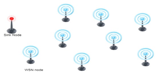
Figure 1. WSN structure.

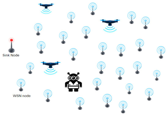
Figure 2. Modernized Wireless Sensor Network (WSN).

To process the sensed data and transmit it to various locations, many nodes must be appropriately deployed. Hence, the minimum number of nodes to be deployed to attain full coverage is enormous [1,2,3,4,5,6,7].

The deployment of nodes is a fundamental but critical aspect that affects the WSN’s performance. Certain nodes are placed randomly, while others are distributed deterministically. In general, random node deployment is preferred in harsh environmental or hostile situations. The deployment of nodes should be done by considering some crucial parameters such as connectivity, coverage, and energy consumption. The Field of Interest (FoI) is declared fully covered if every region’s pixel is covered by a node or more. Nodes are designed to detect events in their sensing ranges and pass the event data to the sink node(s). Communication range defines the range across which nodes communicate with one other. When a network is configured with at least one route to the sink node from each deployed node, it is said to be connected. The WSN is supposed to have coverage with full connectivity for better performance [1].

Power limitation is considered as the one of the critical challenges of WSNs. Since WSNs are often deployed in remote areas such as deserts, forests, or military zones, their nodes are usually powered by AA batteries with a limited lifetime. Recharging such batteries may not be feasible. Some of these nodes could be stationary, while others could be mobile. With the previously stated constraint, nodes lifetime depends on the its energy source.

Consequently, it is highly required for any deployment algorithm to employ nodes’ available energy when selecting which node to move. These node failures can cause areas in the FoI to become devoid of sensor coverage. These areas are called coverage holes. Depending on these coverage holes’ severity, they can degrade performance or disrupt the network entirely [7,8].

Considering the network coverage goal, the highest priority areas or zones should be covered by at least one node. In WSN with mobile nodes, moving a node to high priority zones, more distance to that zone leads to more consumed energy during the movement. Hence, the closer a node it is to the target zone, the better performance in terms of energy efficiency. Therefore, considering the movement distance in the design of the deployment algorithm is highly required.

As in the WSN with mobile nodes, the node deployment referees to finding the optimal possible location of such mobile nodes, covering n-target zones with the minimum number of nodes, are proved to be an NP-complete problem [9]. To address the deployment problem, nature-inspired algorithms were developed. Swarm Intelligence (SI) technique is one of these algorithms being explored to solve WSN problems via efficient optimization. They are very efficient in solving complex problems through simple behavior. One of the most used SI techniques is Ant Colony Optimization (ACO), as it is highly efficient and performs well in a complex environment. The ACO imitates the swarms’ behavior of social ants. Mainly, ants use pheromone as a chemical messenger, and the pheromone concentration can also be interpreted as the solution quality indicator of different interesting issues. Hence, it is possible to describe each mobile node’s motion with ACO [9,10,11,12].

The motivation behind this work is the advances of wireless network technology, including Unmanned ariel vehicles and robotics. These advances in technologies lead to a new generation of wireless networks that combine various types of sensing technologies, robotics, and UAVs. This combination is beneficial in different applications; also, new challenges are generated. One of these challenges is the deployment problem, especially when heterogeneous devices are deployed on a large scale. This paper is a step towards an efficient solution to the deployment problem. This paper studies the sensor relocation problem in WSN to maximize network coverage, considering three key aspects: nodes’ residual energy, movement distance, and movement consumed energy. Therefore, the main contributions of this paper focus on:

(1)

Describing the deployment problem in the form of 0/1 integer programming,

(2)

Considering heterogeneous sensor deployment, including mobile nodes such as robots or UAVs,

(3)

Taking into consideration the zone priority to decide a new location of each node,

(4)

Considering the nodes’ residual energy when selecting which node to move,

(5)

Considering the movement distance and energy to minimize network overall energy consumption.

Finally, developing the Swarm Intelligence algorithm as a near-optimal solution for large-scale deployment problems in reasonable running time enables the use of such algorithms in applications that require real-time sensor relocation.

The paper is laid out as follows: some examples of the related work are given in Section 2. The sensor deployment problem is described in Section 3. The optimal solution approach for this problem is elaborated in Section 4, whereas Section 5 states that the solution being suggested to address deployment problem. The performance results are discussed later in Section 6, and the paper is concluded in Section 7.

2. Related Work

Since this paper’s main objective is to maximize network coverage, this section starts with the classification of the coverage models followed by the coverage classification in WSNs. Then, it discusses some design issues in WSNs for coverage problems such as the deployment methods, sensor node types, mobility of sensor nodes, and solution approaches. In addition, it describes the algorithms that are mostly related to the proposed solutions presented in [6,13], and it discusses the differences from our proposal as well. Finally, the proposal is compared to the research accomplished in [6,13].

Many academics have studied the coverage issue in recent years. The binary and probabilistic models are presented in the literature. The binary model Coverage applies a consistent probability of event detection. Also, the binary coverage probability for a given location p is determined by equation [14]:

$$Cp(p,s)=\left\{\begin{array}{ccc}1\hfill & & if d(s,p)\le r_s\hfill \\ 0\hfill & & \mathit{otherwise}\hfill \end{array}\right.$$

(1)

where sensor node’s sensing range is represented by r_s, the Euclidean distance is represented by d(s,p) and the deployment point is represented by p.

The probabilistic coverage model, in which the probability of monitoring the events has been included, has to use more higher accuracy. WSNs’ coverage may be categorized as [14]:

(1)

Area Coverage

(2)

Target Coverage

(3)

Barrier Coverage

Area coverage focuses on actively monitoring the region of interest. Sensors that are placed randomly are shown in Figure 3a. Each circle depicts the sensing range of a sensor node. Conversely, point coverage concentrates on monitoring a region of interest. Target coverage is shown in Figure 3b. Three sensor nodes observe three targets, t₁, t₂, and t₃, whereas all other targets, t₄ and t₅, are monitored by two sensor nodes. Additionally, target coverage saves energy and reduces the number of nodes required.

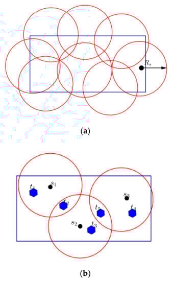
Figure 3. Coverage of the FoI. (a) Area coverage. (b) Target coverage [14].

Overall, barrier coverage is important to monitor for unauthorized border intrusion, see Figure 4 for a summary of the barrier coverage classifications. Weak barrier coverage consists of a few uncovered areas or gaps that may lead to the target being undiscovered. Also, the second category (Strong Barrier Coverage) consists of barrier coverage that improves the sensor nodes’ ability to track or monitor intruders, thereby increasing security [14].

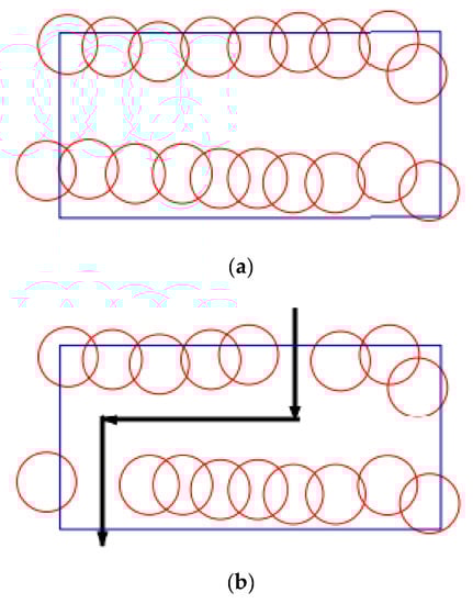
Figure 4. Barrier coverage of the FoI. (a) Strong barrier coverage. (b) Weak barrier coverage [14].

Deployment problems may be deterministic and random deployment. According to Figure 5a, deterministic deployment determines the nodes’ coordinates prior to their actual distribution. Sensor nodes’ positions are set to reduce network costs, energy consumption, high levels of target monitoring, and sensor network lifetimes. However, many applications disallow the adoption of a deterministic approach because of hostile environments or deployment costs. In these situations, random deployment is used. Randomly, Nodes are spread throughout the FoI, as illustrated in Figure 5b. Therefore, the WSN is expected to function better if sensor nodes are deterministically placed rather than randomly deployed [1,14].

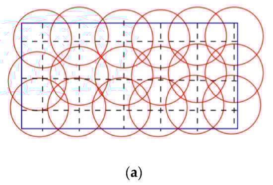
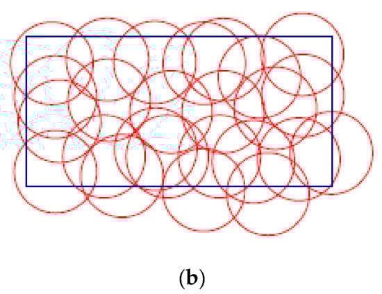
Figure 5. Deployment in WSNs (a) Deterministic deployment. (b) Random deployment [14].

Homogeneous and heterogeneous sensor nodes are two classifications of sensor node types. In homogenous WSNs, sensors are having the same characteristics with respect to sensing range, communication range, energy, and storage. Homogeneous WSNs’ coverage and connection have been examined in many of the literatures [15,16,17,18,19]. Nonetheless, maintaining the homogeneity in WSNs is neither possible nor practical, given certain constraints. The first concern is the cost of WSNs, since the high processing power needed for complicated activities results in a costly sensor node. The cost-effectiveness of a WSN is best shown by include both expensive and cheap sensor nodes. The second challenge is how to deploy sensor nodes once the system is in operation. When it comes to WSNs, heterogeneous sensor nodes are the most important. The ranges of sensor nodes may vary to meet the needs of WSNs. While this adjustment helps lower energy use, it also introduces heterogeneity within WSNs.

Authors of [13] proposed a weight-aware sensor deployment method based on each sensing grid’s weight. The sensor grid is evaluated using Seesaw mapping to reflect factors that include the risk of abnormalities, their consequences, and the time it takes to tolerate such incidents. In order to get an optimum balance between reliability, the existence of field obstacles, and the number of sensors, several weight-aware sensor deployment algorithms are developed to address each of these criteria. However, sensor nodes have important characteristics that these algorithms do not account address. Some sensor nodes use more energy, the number of times may switch from on to off or vice versa, and the number of movements. The lifespan of sensor nodes is a critical challenge in WSN since its operation is highly dependent on such nodes. Indeed, neglecting the decrease in node lifetime caused by its movement across the various zones and its status transitioning from on to off may decrease network performance.

In the context of time-varying differential surveillance requirements, the authors of [6] presents a modelling framework for heterogeneous sensor deployment. It first formulates the problem as an optimization problem using a mixed-integer mathematical programming to maximize field coverage. This is accomplished by using two meta-heuristics. The first heuristic solution uses a Genetic Method (GA), while the second heuristic solution utilizes a Simulated Annealing (SA) algorithm. This framework was created to support large-scale surveillance operations, including integrating multiple sets of heterogeneous sensors into a single deployment strategy.

The sensors’ main characteristics such as energy, allowed number of state-switching, allowed number of moves, and reliability are considered. Meanwhile, the analysis of the proposed framework in [6] shows that the movement distance and movement consumed energy are not considered. This might have a negative influence on network performance, as described above.

A two Flower Pollination Algorithms (FPA) are proposed in [20] to solve the heterogeneous node deployment optimization problem in WSNs with obstacles in the monitoring area. Due to the shortcomings of FPA, such as the low convergence speed and the precision, different enhancements are proposed [20]. The first algorithm is called an Improved Flower Pollination Algorithm (IFPA), while the second algorithm is the Non-dominant Sorting Multi-Objective Flower Pollination Algorithm (NSMOFPA). Via simulation results, the NSMOFPA proved to have a good optimization effect and can provide a better solution for WSN deployment [20].

The optimal sensor deployment problem to minimize sensing uncertainty with a network lifetime constraint is presented in [21]. The authors considered both homogeneous and heterogeneous mobile WSNs. They also consider connectivity to make its model more practical and minimize the sensing uncertainty in a homogeneous network. Two centralized sensor relocation algorithms were designed: centralized constrained movement Lloyed algorithm and Backwards-stepwise centralized constrained movement Lloyed algorithm. A primary goal is to make it easier to balance the trade-off between uncertainty sensing and network lifespan [21].

This paper focuses on how to deploy heterogeneous sensor networks with varying surveillance requirements over time. The problem is mathematically formulated as a 0/1 integer linear programming (ILP) to maximize the area coverage. Then, a meta-heuristic method called Ant-Colony optimization is proposed for large-scale deployment problems.

Like the previous work in [6], this paper considers sensor nodes’ main characteristics such as energy, allowed number of state-switching, and allowed number of moves. Also, as the previous work in [13], the movement distance is considered to improve sensor nodes’ lifespan, improving the overall network performance. In the proposed solution, at each mobile node, the probability of choosing the next deployment point is based on local data, which refers to the movement distance, the residual energy, and the priority of the target zone. Table 1 provides an overall comparison of the two algorithms mentioned earlier [6,13] and the proposed one.

Table 1. A comparative summary of the algorithms mentioned above and the proposed ones.

Paper ID	Parameters
	Residual Energy	Movement Consumed Energy	Movement Distance	Areas (Zones) Priority
[6]	√	×	×	√
[13]	×	×	√	√
Proposed Algorithm	√	√	√	√

3. Problem Description

Consider a field F(A) to be monitored for a time horizon T using a set of sensor nodes, TN. This monitored field is divided into a number of zones A. Each zone i ∈ A is associated with a time-varying weight function ${\omega }_i^t$, where t ∈ T. This weight function quantifies the significance of observations (surveillance requirement) in this zone above horizon T. The sensor nodes are assumed to be stationary or mobile, where the stationary node is assumed to remain in its zone for the entire lifetime. On the contrary, the mobile node can cover multiple zones over time horizon T. The paper’s primary goal is to find the optimum location of the mobile nodes to optimize field coverage. Maximum data coverage is obtained when the highest importance values are collected. The coverage is also maximized by serving a zone with only one node at any given time and keeping the sensor nodes active as much as possible. More importantly, mobile nodes should be used just for as long as they are necessary for sensor node energy conservation. The Movement of the node must occur while minimizing the distance between the node’s position and the new location.

4. Problem Formulation for Optimal Solution

Our previous modelling indicates that the deployment problem can be solved optimally. Optimal solution will help in producing an efficient heuristic. This problem is mathematically formulated using ILP. Although this solution is used to confirm the optimal solution and fully understand the problem with its major constraints, it is intractable to solve large-scale problems in terms of the elapsed time and/or memory required for problem-solving. Hence, the ILP solution is utilized to solve small-scale problems and guarantee the proposed solution’s efficiency.

To fully understand the used notations used in our solutions, the reader is referred to Table 2 for the meaning of each symbol used in the formulation.

Table 2. Deployment problem model notations.

Given Parameters
Notation	Description
S	The set of all mobile nodes.
A	The set of all zones in the monitored field.
T	The time horizon.
TN	The set of all stationary and mobile nodes in the monitored field.
${\omega }_i^t$	The time-varying weight function for each zone $i\in A$, where $t\in T$.
$M_s$	The maximum number of moves allowed for such node s, $s\in S$.
$P_s$	The maximum number of switches allowed for such node s, $s\in S$.
$d_{sij}^t$	Is the Euclidean distance between the location of node s on zone i and its new location on zone j(center of zone j), where $i,j\in A$, $s\in S$ and $t\in T$.
$E_{sij}^t$	The energy required for the movement of node s from zone i to zone j at time interval t, where $i,j\in A$, $s\in S$ and $t\in T$.
$E{S}_s$	The energy required for changing the state of node s from off to on $s\in S$.
$R{E}_s^t$	Is the residual energy of node s at time interval t, where $s\in S$ and $t\in T$.
Indicator Parameter
${\delta }_{si}^t$	1 if node s is on zone i at time t and 0 otherwise.
Decision Variables
$x_{si}^t$	1 if node s exists in active state on zone i at time interval t, and 0 otherwise, $\forall s\in S,\forall i\in A,\forall t\in T$.
$y_{si}^t$	1 if node s exists in inactive state on zone i at time interval t, and 0 otherwise, $\forall s\in S,\forall i\in A,\forall t\in T$.
$m_{sij}^t$	1 if node s is moved from zone i to zone j at time interval t, and 0 otherwise, $\forall s\in S,\forall i,j\in A,\forall t\in T$.
$o{n}_{si}^t$	1 if node s is turned to active state at time interval t on zone i, and 0 otherwise, $\forall s\in S,\forall i\in A,\forall t\in T$.
$of{f}_{si}^t$	1 if node s is deactivated at time interval t on zone i, and 0 otherwise, $\forall s\in S,\forall i\in A,\forall t\in T$.
$g_i$	1 if the number of all nodes on zone i is greater than one node at time interval t, and 0 otherwise, where $i\in A$ and $t\in T$.
$N_j$	1 if the number of all nodes on zone j is greater than zero at time interval t, and 0 otherwise, where $j\in A$ and $t\in T$.
$Z_n$	1 if the difference the distance of n and s is less than zero and 0 otherwise, where $n,s\in S$.
$e_{\upsilon }$	1 if the difference between the residual energy of s at time interval t is less than that of node υ and 0 otherwise, where $\upsilon ,s\in S$, and $t\in T$.
$s{p}_{ij}$	1 if the number of nodes on zone i is greater than one node at time t, and the weight of zone j is less than that of zone i, and 0 otherwise, $i,j\in A$.

As can be seen in Equation (2), the objective function maximizes the field coverage described as the sum over all time intervals of the products of the observation weight ${\omega }_i^t$ and the decision variable $x_{si}^t$.

$$The overall field c\mathrm{overage}={\displaystyle \sum _{t\in T}{\displaystyle \sum _{i\in A}{\displaystyle \sum _{s\in S}{\omega }_i^t}}}{x}_{si}^t$$

(2)

Based on this computation, the objective function is defined by the following equation:

$$Z_{IP}=\mathbf{max}{\displaystyle \sum _{t\in T}{\displaystyle \sum _{i\in A}{\displaystyle \sum _{s\in S}{\omega }_i^t}}}{x}_{si}^t (\mathrm{IP})$$

Subject to:

$$x_{si}^t+y_{si}^t\le 1\hspace{1em}\hspace{1em}\hspace{1em}\hspace{1em}\forall s\in S,\forall i\in A,\forall t\in T$$

(3)

$$1-\left({\displaystyle \sum _{j\in A}{x}_{sj}^{t+1}}+{\displaystyle \sum _{j\in A}{x}_{sj}^{t-1}}\right)\ge x_{si}^t\hspace{1em}\forall s\in S,\forall i\in A,\forall t\in T$$

(4)

$${\displaystyle \sum _{i\in A}{x}_{si}^t}\le 1\hspace{1em}\hspace{1em}\hspace{1em}\hspace{1em}\forall s\in S,\forall t\in T$$

(5)

$$x_{si}^{t+1}{y}_{si}^t\le m_{sij}^t\hspace{1em}\hspace{1em}\hspace{1em}\hspace{1em}\forall s\in S,\forall i\in A,\forall t\in T$$

(6)

$$1-\left(y_{si}^{t+1}\cdot x_{si}^t\right)\ge m_{sij}^t\hspace{1em}\hspace{1em}\hspace{1em}\hspace{1em}\forall s\in S,\forall i\in A,\forall t\in T$$

(7)

$${\displaystyle \sum _{i\in A}{\displaystyle \sum _{j\in A}{\displaystyle \sum _{t\in T}{m}_{sij}^t}\le M_s}}\hspace{1em}\hspace{1em}\hspace{1em}\hspace{1em}\forall s\in S$$

(8)

$$g_i{\displaystyle \sum _{s\in S\cup TN}{\delta }_{si}^t}>1\hspace{1em}\hspace{1em}\hspace{1em}\hspace{1em}\forall s\in S,i\in A,t\in T$$

(9)

$$g_i\le m_{sij}^t\hspace{1em}\hspace{1em}\hspace{1em}\hspace{1em}\forall s\in S,\forall i,j\in A,\forall t\in T$$

(10)

$$N_j{\displaystyle \sum _{s\in S\cup TN}{\delta }_{sj}^t}>0\hspace{1em}\hspace{1em}\hspace{1em}\hspace{1em}\forall s\in S,j\in A,t\in T$$

(11)

$$2-N_j=m_{sij}^t+1\hspace{1em}\hspace{1em}\hspace{1em}\hspace{1em}\forall s\in S,\forall i,j\in A,\forall t\in T$$

(12)

$$s{p}_{ij}{\displaystyle \sum _{s\in S\cup TN}{\delta }_{si}^t}>1\hspace{1em}\hspace{1em}\hspace{1em}\hspace{1em}\forall s\in S,\forall i,j\in A,\forall t\in T$$

(13)

$$s{p}_{ij}\cdot {\omega }_i^t>{\omega }_j^t\hspace{1em}\hspace{1em}\hspace{1em}\hspace{1em}\forall s\in S,\forall i,j\in A,\forall t\in T$$

(14)

$$s{p}_{ij}\le m_{sij}^t\hspace{1em}\hspace{1em}\hspace{1em}\hspace{1em}\forall s\in S,\forall i,j\in A,\forall t\in T$$

(15)

$${\displaystyle \sum _{s\in S}{m}_{sij}^t}\le 1\hspace{1em}\hspace{1em}\hspace{1em}\hspace{1em}\forall t\in T,\forall i,j\in A$$

(16)

$$y_{si}^{t-1}\le o{n}_{si}^t\hspace{1em}\hspace{1em}\hspace{1em}\hspace{1em}\forall s\in S,\forall i\in A,\forall t\in T$$

(17)

$$1-x_{si}^{t+1}\ge o{n}_{si}^t\hspace{1em}\hspace{1em}\hspace{1em}\hspace{1em}\forall s\in S,\forall i\in A,\forall t\in T$$

(18)

$$x_{si}^{t-1}\le of{f}_{si}^t\hspace{1em}\hspace{1em}\hspace{1em}\hspace{1em}\forall s\in S,\forall i\in A,\forall t\in T$$

(19)

$$1-y_{si}^{t+1}\ge of{f}_{si}^t\hspace{1em}\hspace{1em}\hspace{1em}\hspace{1em}\forall s\in S,\forall i\in A,\forall t\in T$$

(20)

$${\displaystyle \sum _{t\in T}{\displaystyle \sum _{i\in A}\left(o{n}_{si}^t+of{f}_{si}^t\right)}}\le P_s\hspace{1em}\hspace{1em}\hspace{1em}\hspace{1em}\forall s\in S,\forall i\in A,\forall t\in T$$

(21)

$${\displaystyle \sum _{n\in S-\left\{s\right\}}{Z}_n\left(d_{nij}^t-d_{sij}^t\right)}<0\hspace{1em}\hspace{1em}\hspace{1em}\hspace{1em}\forall s\in S,\forall i,j\in A,\forall t\in T$$

(22)

$$2-{\displaystyle \sum _{n\in S-\left\{s\right\}}{Z}_n}=m_{sij}^t+1\hspace{1em}\hspace{1em}\hspace{1em}\hspace{1em}\forall s\in S,\forall i\in A,\forall t\in T$$

(23)

$${\displaystyle \sum _{n\in S-\left\{s\right\}}{Z}_n\le 1}\hspace{1em}\hspace{1em}\hspace{1em}\hspace{1em}\forall s\in S$$

(24)

$$m_{sij}^t\left(R{E}_s^t-E_{sij}^t\right)\ge E_{th}\hspace{1em}\hspace{1em}\hspace{1em}\hspace{1em}\forall s\in S,\forall i,j\in A,\forall t\in T$$

(25)

$${\displaystyle \sum _{\upsilon \in S-\left\{s\right\}}{e}_{\upsilon }\left[\left(R{E}_s^t-E_{sij}^t\right)-\left(R{E}_{\upsilon }^t-E_{\upsilon ij}^t\right)\right]<0\hspace{1em}\hspace{1em}\hspace{1em}\hspace{1em}\forall s\in S,\forall t\in T}$$

(26)

$$2-{\displaystyle \sum _{\upsilon \in S-\left\{s\right\}}{e}_{\upsilon }}=m_{sij}^t+1\hspace{1em}\hspace{1em}\hspace{1em}\hspace{1em}\forall s\in S,\forall i,j\in A,\forall t\in T$$

(27)

$${\displaystyle \sum _{\upsilon \in S-\left\{s\right\}}{e}_{\upsilon }}\le 1\hspace{1em}\hspace{1em}\hspace{1em}\hspace{1em}\forall s\in S$$

(28)

$$o{n}_s^t\left(R{E}_s^t-E{S}_s\right)\ge E_{th}\hspace{1em}\hspace{1em}\hspace{1em}\hspace{1em}\forall s\in S,\forall t\in T$$

(29)

$$\begin{array}{c}\left\{x_{si}^t,y_{si}^t,m_{sij}^t,o{n}_{si}^t,of{f}_{si}^t,Z_n,e_{\upsilon },s{p}_{ij}\right\}=1 or 0\hfill \\ \hfill \forall s\in S,\forall i,j\in A,\forall t\in T\end{array}$$

(30)

For the reader to understand the constraints, they are divided into groups and described below:

(1) 

Deployment Constraints:

The deployment constraints involve the following:

(a)

The constraint in Equation (3) is utilized to ensure that any mobile node s is either in an active or inactive state during any time interval.

(b)

The constraint in Equation (4) is used to determine the value of the decision variable $x_{si}^t$. The sensor node s is set to be active in zone i during time interval t, $x_{si}^t$ is enforced to 1, If that node is not used in any zone j during the next and previous time intervals.

(2) 

Assignment Constraint:

This constraint is utilized to ensure that any mobile node s is covering at most one zone at each time interval, as given in Equation (5).

(3) 

Mobility Constraints:

The mobility constraints are used to determine if the node s is moved from zone i to zone j at the end of interval t. They involve the following:

Equations (6) and (7) constraints compare zones where mobile node s is deployed during time intervals t and t + 1. The decision variable $m_{sij}^t$ is enforced to 1 if they are different.

(a)

The constraint in Equation (8) is used to ensure that the number of moves made by any node s is less than or equal to the maximum number of moves allowed for that node.

(b)

The constraints in Equations (9) and (10) guarantee that the movement of a node s from zone i to zone j does not make zone i empty.

(a)

Equations (11) and (12) ensure that the zone j which the node s will move to is not covered by any node, whether stationary or moving node.

(b)

The constraints in Equations (13)–(15) handle a special case in which the number of nodes in zone j is 0 but ${\omega }_j^t<{\omega }_i^t$.

(c)

The constraint in Equation (16) ensures that the number of moves made by a mobile node s during time interval t should be less than or equal to 1.

(1) 

State-Switching Constraints:

The state-switching constraints involve the following:

(a)

The constraints in Equations (17)–(20) determine the state switching of a sensor node from active to inactive state and vice versa.

(b)

For each mobile node, the total number of state switching should be less than or equal to the maximum number of switches allowed for such node as given in Equation (21).

(2) 

Distance Constraints:

The distance constraints are designed to guarantee that moved node s from zone i to zone j is close as much as possible to zone j. That’s to say, the selected mobile node s has the minimum distance between its location on zone i and the new location at the centre of zone j as illustrated in Equations (22)–(24).

(3) 

Energy Constraints:

The energy constraints illustrated in Equations (25)–(29) are used to conserve energy and prolong the network lifetime. They involve the following:

(a)

The mobile node s is utilized when its expected residual energy after the movement from zone i to zone j is greater than or equal to the threshold value, and it has the maximum expected residual energy compared to the others at the same time as given in Equations (25)–(28).

(b)

The state of the mobile node s is changed from off to on when its residual energy after the state-switching is greater than or equal to the threshold value, as illustrated in Equation (29).

(4) 

Decision Variable Constraint:

The decision variable constraint is illustrated in Equation (30), where all the decision variables are equal to 0 or 1.

(5) 

Walk-Through Example:

In this section, a simplified example shown in Figure 6 is explained walking through node deployment step by step to understand better how the constraints work and how the optimal deployment is performed. The example is used to illustrate the deployment of four sensors, S₁, S₂, S₃, and S_4, of four zones Z₁, Z₂, Z₃, and Z₄, which is monitored for two-time intervals t₁ and t₂. Table 3 shows the residual energy of each sensor node before and after movement, providing the movement distance and residual energy.

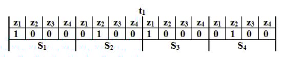
Figure 6. Initial deployment before the movement operation.

Table 3. Parameters of mobile sensor nodes.

Sensor Nodes	Residual Energy	Movement Distance		Movement Required Energy		Residual Energy after Movement
		Z3	Z4	Z3	Z4	Z3	Z4
S1	10 J	10 m	40 m	10 J	40 J	0 J	Not enough
S2	7 J	30 m	5 m	30 J	5 J	Not enough	2 J
S3	15 J	10 m	30 m	15 J	30 J	5 J	Not enough
S4	20 J	25 m	20 m	25 J	20 J	Not enough	0 J

Figure 6 represents the initial deployment of the four sensors at the first-time interval, t₁. Assume that relation between the priority of each zone and the others during the second time interval t₂, is described as ${\omega }_1^{t_2}<{\omega }_3^{t_2}<{\omega }_2^{t_2}<{\omega }_4^{t_2}$.

Three combinations of the proposed optimal solution parameters are selected, listed in Table 4, to understand and evaluate their effects on network performance. We refer to these parameter combinations as Case 1–3, respectively.

Table 4. Proposed parameter combinations.

Combination	Parameters
	Zone Priority	Residual Energy	Movement Distance	Movement Consumed Energy
Case 1	√	×	√	×
Case 2	√	√	×	×
Case 3	√	√	√	√

As the field coverage is used as the optimization function, all cases consider the weight function for each zone, ${\omega }_i^t$ (zone priority). Regarding Case 1, the deployment point is only determined by the zone priority and the movement distance, making the zone with the highest priority and the shortest movement distance is selected as the candidate deployment point. Figure 7a shows the movement operation during the time interval, t₂, under the parameter combination of Case 1. Aiming to maximize field coverage and minimize movement distance, the deployment patterns of S₁ and S₂ are exchanged over the entire horizon (t₁ and t₂). Now, the residual energy of S₁ is zero, which impacts the network lifetime and the proper operation of the WSN. In Case 2, besides the zone priority, the deployment decision is also affected by residual energy to avoid poor-energy nodes. Thus, avoiding poor-energy nodes to improve network lifetime is its second priority. Figure 7b shows the movement operation during the time interval, t₂, under parameter combination of Case 2. The deployment patterns of sensor nodes S₃ and S₄ are swapped over time periods t₁ and t₂ for field coverage maximization and energy saving. Now that S₄ has no residual energy, depending on it alone to increase energy efficiency will be insufficient.

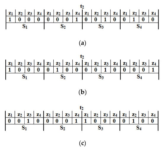
Figure 7. The movement operation during the time interval, t₂ under various parameter combinations (a) Case 1, (b) Case 2, and (c) Case 3.

Finally, in Case 3, besides zone priority and the movement distance, the expected residual energy after the movement is added to improve energy efficiency. Figure 7c shows the crossover operation during the time interval, t₂, under the parameter combination of Case 3. Aiming to maximize field coverage and energy efficiency, the deployment patterns of sensor nodes S₂ and S₃ are exchanged during the time intervals t₁ and t₂. Here, the residual energy on S₂ and S₃ are 2 J and 5 J, respectively. Thus, it is possible to observe that considering the expected residual energy after the movement, the movement distance and zone priority into deployment decision turn into much better energy efficiency than the other cases.

5. Ant Colony Optimization Based Solution

This section deals with the second solution developed for the deployment problem, the ACO technique. In ACO [22,23,24], to find a solution to the deployment problem, ants build solutions incrementally by walking randomly through a connected graph G(P,E), where P denotes the set of the deployment points and E represents a set of all undirected links connecting the deployment points and the sink node. To construct a solution to the deployment problem, each ant k starts its tour at each mobile node location and then consecutively builds the connected covers through transitioning among the deployment points in the construction graph. At each tour construction step, ant k applies a probabilistic transition rule to select which deployment point it will visit next. The probability that ant k, currently at deployment point p_i, i = 0, 1, …, |P|, will select deployment point p_j, j = 1, 2, …, |P|, to visit next is given by:

$$P_{ij}^k(t)=\left\{\begin{array}{ll}\frac{{\left[{\tau }_{ij}(t)\right]}^{\alpha }{\left[{\eta }_k(t)\right]}^{\beta }{\left[{\psi }_j(t)\right]}^{\gamma }}{{\displaystyle \sum _{l\in A}{\left[{\tau }_{il}(t)\right]}^{\alpha }{\left[{\eta }_k(t)\right]}^{\beta }{\left[{\psi }_l(t)\right]}^{\gamma }}}& if {\delta }_{sj}^t=0\\ 0& \mathit{otherwise}\end{array}\right.$$

(31)

where ${\tau }_{ij}(t)$ is the pheromone value between deployment point d_i and d_j at the time t, ${\eta }_k(t)$, and ${\psi }_j(t)$ are the heuristic information; α, β, and γ are the weight factors that control the pheromone value and the heuristic information parameters respectively.

A. 

Pheromone calculation

In this paper, the pheromone concentration is affected by the distance between each mobile node’s location and its new location on the target zone since energy conversation is an essential issue in WSN. The mobile node selection with minimum distance is required to minimize energy consumption in the movement and, hence, conserve much more energy as possible. Thus, the distance between the location of node s on zone i and the new location on the target zone j is used to calculate the increasing density of pheromone value as follows:

$$\Delta {\tau }_{ij}=d_{sij}^t$$

(32)

After each ant, k, has reached its new deployment point, the pheromone trail value is updated according to the following rule:

$${\tau }_{ij}(t)=(1-\rho ){\tau }_{ij}(t-1)ij+\rho \Delta {\tau }_{ij}$$

(33)

where $\rho \in \left(0,1\right)$ is the evaporation factor [25].

B. 

Calculation of the heuristic information

To maximize field coverage, the observation weight of the target zone is used as heuristic information when selecting the next deployment point, which denoted by:

$${\psi }_j(t)=\frac{{\omega }_j(t)}{{\displaystyle \sum _{l\in A}{\omega }_l(t)}}$$

(34)

The candidate zone that has a greater value of ${\psi }_j(t)$ meaning that zone has a higher priority and will have a better opportunity to be the chosen target zone.

As the conversation is a critical issue in WSNs, any mobile node with less energy than its required energy for the movement should not be utilized. Therefore, the heuristic value of moving a certain mobile node from deployment point i to j by ant k, denoted by ${\eta }_k(t)$, is directly proportional to remaining energy after the movement as follows:

$${\eta }_k(t)=\frac{\left(R{E}_k^t-E_{kij}^t\right)}{{\displaystyle \sum _{l\in K}\left(R{E}_l^t-E_{lij}^t\right)}}$$

(35)

The ant that has a higher value of ${\eta }_k(t)$ meaning that the mobile node where such an ant will have higher residual energy in case it has been moved from deployment point i to j, the deployment point j has more chance to be the next deployment point.

6. Performance Evaluation

In this section, different sets of numerical simulation experiments are conducted to demonstrate our proposed heuristic performance. This section first introduces the evaluation criteria. Then, it describes the evaluation methodology. Finally, the section presents the simulation results and comparisons with benchmarks.

A. 

Performance Criteria

We evaluate E3AF using the following criteria:

(1)

Network Lifetime [26] is the period from the start of network operations to the first failed node due to battery depletion.

(2)

Coverage Ratio is very essential in our deployment method. That is reasonable since our main goal is to increase network coverage. The coverage ratio is defined as the number of zones covered with at least one sensor node. In this context, the highest priority zones should be covered as much as possible.

$$Coverage Ratio=\frac{{\displaystyle \sum _{i=1}^{n}Z{p}_i}}{{\displaystyle \sum _{j=1}^{m}Z{p}_j}}$$

(36)

where m is the total number of zones, Zp_i is the zone’s i priority, and n is the number of covered zones.

B. 

Methodology

To comprehensively validate the proposed deployment algorithm, a series of experiments are carried out using the MATLAB simulator. The experiments are carried out using an Intel Core i5 dual-core CPU with a frequency of 2.3 GHz, 4 GB of memory, and a Windows 7 operating system. 300 × 300 m square region is considered, where N sensor nodes are deployed to monitor the area. Such sensor nodes are divided into mobile and stationary nodes. The stationary nodes are deployed randomly in a monitored field, and the sink node is placed at (300 m, 0 m). We provide the simulation results for the heterogeneous network, including sensor nodes with different sensing and battery energies. The initial energy of each sensor node is set between 1 to 19,160 J. it is assumed that a 35 m sensing range and the energy consumption during node movement is 1 J/m [8,27].

As for sensing, it is assumed that each sensor acquires 1 KB of data per second. According to [8], the energy dissipation for data acquisition is defined in Equation (37), where NB is the number of bytes of data acquired. P_dac is the required power for data acquisition, and D_so is the duration of a single operation. In this work, we have adopted the same values in [8]. NB = 1 KB, D_so = 0.135 µs, and P_dac = 300 mW.

$$E_{acq}=NB{P}_{dac}{D}_{so}$$

(37)

As for data communication between two nodes, we have adopted the energy consumption model, and the model of lossy links in WSNs is based on [28]. Besides, each node runs the AODV routing protocol [29] to send and forward data packets. When running simulation, data traffic in the network is generated according to a Poisson process with a mean parameter, λ. The simulation parameters are listed in Table 5.

Table 5. Simulation environment parameters [8,27].

Parameters	Values
Network size	300 m × 300 m
Number of sink nodes	1
Maximum number of retransmission	4
Packet size	50 byte
Data rate	19.2 Kbps
Frequency	868 MHz
Transmission power	0 dBm
Maximum transmission range	200 m
Path loss exponent	3
Shadow fading variance	4
Noise power	−141 dBm
Reference distance	1 m
λ	15

C. 

Results and Discussion

The suggested deployment method was evaluated with respect to network lifespan and coverage ratio under various number of mobile nodes, number of sensor nodes, and initial deployment strategies of mobile nodes.

(1)

Network Lifetime Evaluation

Here, a set of experiments is conducted to evaluate whether the improved coverage is worth the trade-off in energy consumption which in turn negatively affect the network lifetime. In this set, the performance of the proposed deployment algorithm is evaluated in terms of network lifetime compared to the deployment algorithms in [6,13].

The first experiment studies the variation of network lifetime with a different number of mobile nodes. This experiment varies the percentage number of mobile nodes from 10% to 50% of the overall network nodes. The total number of sensor nodes in the network is set to 90. Figure 8 shows the variation of network lifetime to the percentage of the mobile node.

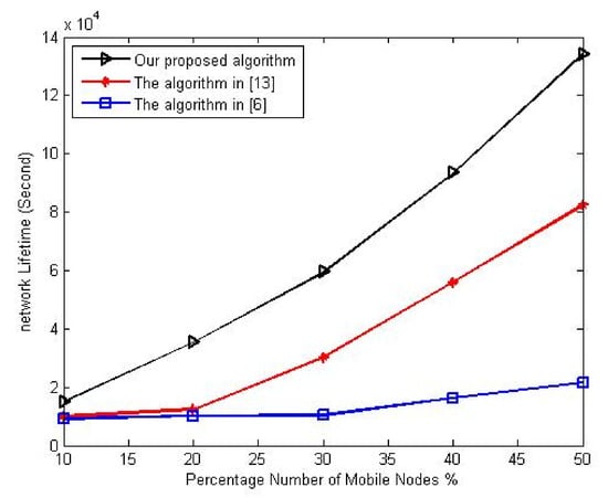
Figure 8. Influence of increasing percentage of mobile nodes on network lifetime.

As seen in Figure 8, the proposed deployment algorithm gives the best improvement in the network lifetime over other algorithms. It employs the nodes’ available energy, movement energy, and movement distance to decide each mobile node’s new location. Meanwhile, the comparison indicates that the deployment algorithm in [13] gives the worst performance since it does not consider nodes’ residual energy when selecting which node to move. Still, it attempts to select only the nodes with the shortest movement distance. On the other hand, the deployment algorithm in [6] does not employ the movement distance, but it selects only nodes with the lowest movement distance.

In the second experiment, the proposed algorithm’s performance is evaluated under different sensor nodes compared to the algorithms in [6,13]. This experiment varies the number of sensor nodes from 90 to 130 nodes while setting mobile nodes’ percentage at 30%. Figure 9 shows the variation of network lifetime with a different number of sensor nodes. From this figure, it can be observed that the proposed algorithm greatly increases the network lifetime in comparison to previous algorithms.

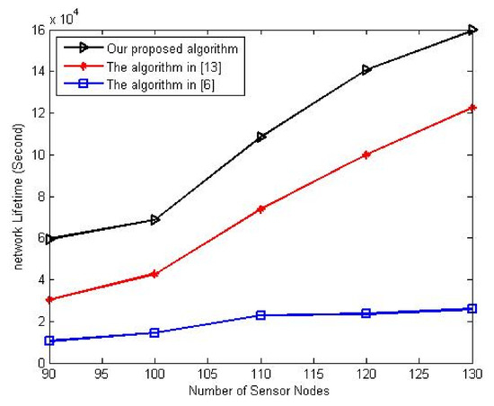
Figure 9. Influence of increasing number of sensor nodes on network lifetime.

In the last experiment of this set, the proposed algorithm’s performance is evaluated with different initial deployment strategies of mobile nodes. We select four strategies for the initial deployment of mobile nodes, listed in Table 6, to evaluate their effects on the network deployment. We refer to these strategies as strategy 1–4, respectively. In this experiment, the number of sensor nodes and the percentage number of mobile nodes is set to 90 and 30%, respectively.

Table 6. Initial deployment strategies.

Strategies	Deployment
Strategy 1	Random Distribution
Strategy 2	At Line along the middle of the network
Strategy 3	At the Network Corners
Strategy 4	Uniform Distribution

Figure 10 shows the variation of network lifetime with different initial deployment strategies of mobile nodes. It is clear from the figure that the best performance is achieved when mobile nodes’ initial deployment is at network corners as locating the mobile nodes at such initial location decreases the movement distance between the mobile nodes and the target zones; thus, it reduces the consumed energy during the movement. However, the proposed algorithm has the best network lifetime compared to other algorithms.

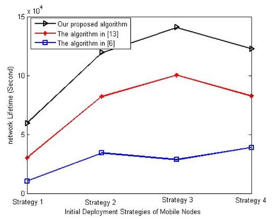
Figure 10. Influence of initial deployment strategy of mobile nodes on network lifetime.

(2)

Coverage Ratio Evaluation

In this set of experiments, we observe each deployment algorithm’s ability to maintain the highest priority zones’ coverage as much as possible. During these experiments, the network’s overall coverage ratio is measured and plotted against the number of mobile nodes, sensor nodes, and deployment approaches.

This research assesses the mobile coverage ratio using various percentages of nodes. The experiment was performed by increasing the percentage of mobile nodes, from 10% to 50%. 90 sensor nodes have been assigned. Figure 11 illustrates the coverage ratio changing according to the percentage of mobile nodes. As clearly seen, the proposed algorithm provides better coverage ratio compared to the deployment algorithm in [13]. However, the deployment algorithm’s main goal in [6] is to improve network coverage, while the primary purpose of the proposed algorithm is to achieve the trade-off between coverage improvement and energy consumption. So, based on these results, we can say that the proposed algorithm achieves the suitable trade-off between the coverage improvement and the network lifetime. On the other hand, the deployment algorithm in [6] cannot get such a reasonable trade-off since it has the lowest coverage ratio.

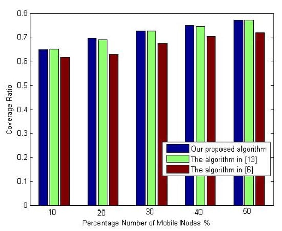
Figure 11. Influence of increasing percentage of mobile nodes on coverage ratio.

The second experiment of this set is conducted to evaluate the proposed algorithm’s performance regarding the coverage ratio against the number of sensor nodes. The comparison again is made against the deployment algorithms in [6,13]. A different number of sensor nodes is utilized. Throughout this experiment, the number of sensor nodes is varied from 90 to 130 nodes. The percentage of the mobile nodes is set at 30%.

Figure 12 examines the coverage ratio with a different number of sensor nodes. As shown in this figure, we can easily observe that the proposed algorithm improves the coverage ratio similar to the deployment algorithm in [13]. At the same time, it outperforms the deployment algorithm in [6] with almost 4%.

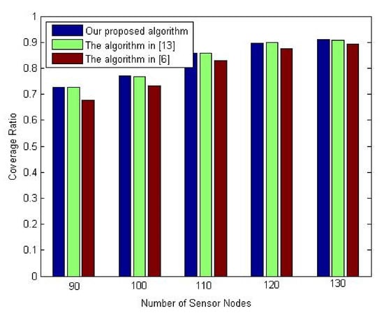
Figure 12. Influence of increasing number of sensor nodes on the coverage ratio.

The third experiment of this set is performed to study the variation of the coverage ratio using mobile nodes’ initial deployment strategies listed in Table 5. This simulation experiment was conducted by fixing the mobile nodes’ percentage and the number of sensor nodes to 30% and 90 nodes.

Figure 13 shows the variation of the coverage ratio with the initial deployment strategies of mobile nodes. It is obvious from this figure that the initial deployment at the network corners gives the best coverage ratio. The reason is the highest priority zones are covered at that initial deployment strategy. However, the proposed algorithm again slightly achieves the same performance as the deployment algorithm in [13], but it outperforms the deployment algorithm presented in [6] with almost 3%.

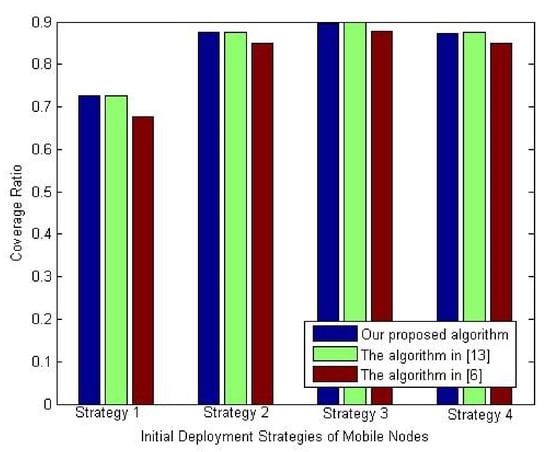
Figure 13. Influence of initial deployment strategy of mobile nodes on coverage ratio.

7. Conclusions

This work introduced an efficient routing algorithm for WSNs for better information fusion. The proposed algorithm considered the environmental conditions and other important parameters such as link load balancing, node energy, and reliability. The algorithms provided a model for the environment conditions where the routing protocol could avoid highly languorous areas. The algorithm is compared to two of the recently published algorithms correcting some of the used equations and adding more realistic parameters to be considered during the routing process. One of the proposed algorithm drawbacks is the time complexity where it takes more time than the other two algorithms that is compared with. However, it is a tradeoff between the performance and time complexity. Another drawback that could be worth mentioning is the uncertainty in the input data due to the inefficiency of the sensor nodes themselves. The future of this research involves the practical implementation of the proposed protocol on real networks. It is planned to implement the proposed algorithm on Altera Cyclone IV FPGA Development Board is one of the best choices for implementation. Other future work includes adding more realistic problems, such as obstacles in the monitoring field. In addition, sensors data is usually unreliable, and it might be noisy or include many redundancies. A fuzzy-based technique might help cleaning the data before it reaches the sink node. Moreover, comparing between a synchronous and asynchronous techniques with different types of networks and sizes could be another extension to the work in this paper.

References

- Priyadarshi, R.; Gupta, B.; Anurag, A. Deployment techniques in wireless sensor networks: A survey, classification, challenges, and future research issues. J. Supercomput. 2020, 76, 7333–7373. [Google Scholar] [CrossRef]
- Mainwaring, A.; Polastre, J.; Szewczyk, R.; Culler, D.; Anderson, J. Wireless sensor networks for habitat monitoring. In Proceedings of the 1st ACM International Workshop on Wireless Sensor Networks and Applications (WSNA’ 02), Atlanta, GA, USA, 28 September 2002; pp. 88–97. [Google Scholar]
- Kuorilehto, M.; Hännikäinen, M.; Hämäläinen, T.D. A survey of application distribution in wireless sensor networks. EURASIP J. Wirel. Commun. Netw. 2005, 2005, 774–788. [Google Scholar] [CrossRef] [Green Version]
- Nguyen, N.T.; Venkatesh, S.; West, G.; Bui, H.H. Multiple camera coordination in a surveillance system. Acta Autom. Sin. 2003, 29, 408–422. [Google Scholar]
- Ramadan, R.; El-Rewini, H.; Abdelghany, K. Optimal and Approximate Approaches for Deployment of Heterogeneous Sensing Devices. EURASIP J. Wirel. Commun. Netw. 2007, 2007, 54731. [Google Scholar] [CrossRef] [Green Version]
- Ramadan, R.; Abdelghany, K.; El-Rewini, H. SensDep: A Design Tool for the Deployment of Heterogeneous Sensing Devices. In Proceedings of the 2nd IEEE Workshop on Dependability and Security in Sensor Networks and Systems, Columbia, MD, USA, 24–28 April 2006. [Google Scholar]
- Obaidat, M.S.; Misra, S. Principles of Wireless Sensor Networks; Cambridge University Press: Cambridge, UK, 2015. [Google Scholar]
- Khalifa, B.; Khedr, A.M.; Al Aghbari, Z. A Coverage Maintenance Algorithm for Mobile WSNs with Adjustable Sensing Range. IEEE Sens. J. 2020, 20, 1582–1591. [Google Scholar] [CrossRef]
- Sarobin, M.V.R.; Ganesan, R. Swarm Intelligence in Wireless Sensor Networks: A Survey. Int. J. Pure Appl. Math. 2015, 101, 773–807. [Google Scholar]
- McCune, R.R.; Madey, G.R. Control of Artifial Swarms with DDDAS. Procedia Comput. Sci. 2014, 29, 1171–1181. [Google Scholar] [CrossRef] [Green Version]
- Nayyar, A.; Singh, R. Ant colony optimization (ACO) based routing protocols for wireless sensor networks (WSN): A survey. Int. J. Adv. Comput. Sci. Appl. 2017, 8, 148–155. [Google Scholar] [CrossRef] [Green Version]
- Yang, X.-S.; Karamanoglu, M. Swarm Intelligence and Bio-Inspired Computation: An Overview. In Swarm Intelligence and Bio-Inspired Computation; Elsevier: Amsterdam, The Netherlands, 2013; pp. 3–23. [Google Scholar]
- Xie, M.; Bai, Y.; Hu, Z.; Shen, C. Weight-Aware Sensor Deployment in Wireless Sensor Networks for Smart Cities. J. Wirel. Commun. Mob. Comput. 2018, 2018, 1–15. [Google Scholar] [CrossRef] [Green Version]
- Tripathi, A.; Gupta, H.P.; Dutta, T.; Mishra, R.; Shukla, K.K.; Jit, S. Coverage and Connectivity in WSNs: A Survey, Research Issues and Challenges. IEEE Access 2018, 6, 26971–26992. [Google Scholar] [CrossRef]
- Alam, S.M.N.; Haas, Z.J. Coverage and connectivity in threedimensional networks. In Proceedings of the MobiCom06: 12th Annual International Conference on Mobile Computing and Networking, Los Angeles, CA, USA, 23–29 September 2006; pp. 346–357. [Google Scholar]
- Aslam, N.; Robertson, W. Distributed coverage and connectivity in three-dimensional wireless sensor networks. In Proceedings of the IWCMC ’10: 2010 International Wireless Communications and Mobile Computing Conference, Caen, France, 28 June–2 July 2010; pp. 1141–1145. [Google Scholar]
- Berman, P.; Calinescu, G.; Shah, C.; Zelikovsky, A. Power efficient monitoring management in sensor networks. In Proceedings of the 2004 IEEE Wireless Communications and Networking Conference (IEEE Cat. No.04TH8733), Atlanta, GA, USA, 21–25 March 2004; pp. 2329–2334. [Google Scholar]
- Boukerche, A.; Fei, X. A Voronoi approach for coverage protocolsin wireless sensor networks. In Proceedings of the IEEE GLOBECOM 2007—IEEE Global Telecommunications Conference, Washington, DC, USA, 26–30 November 2007; pp. 5190–5194. [Google Scholar]
- Gao, J.; Li, J.; Cai, Z.; Gao, H. Composite event coverage in wirelesssensor networks with heterogeneous sensors. In Proceedings of the 2015 IEEE Conference on Computer Communications (INFOCOM), Hong Kong, China, 26 April–1 May 2015; pp. 217–225. [Google Scholar]
- Wang, Z.; Xie, H.; He, D.; Chan, S. Wireless Sensor Network Deployment Optimization Based on Two Flower Pollination Algorithms. IEEE Access 2019, 7, 180590–180608. [Google Scholar] [CrossRef]
- Guo, J.; Jafarkhani, H. Movement-Efficient Sensor Deployment in Wireless Sensor Networks with Limited Communication Range. IEEE Trans. Wirel. Commun. 2019, 18, 3469–3484. [Google Scholar] [CrossRef]
- Elnaggar, O.E.; Ramadan, R.A.; Fayek, M.B. WSN in monitoring oil pipelines using ACO and GA. Procedia Comput. Sci. 2015, 52, 1198–1205. [Google Scholar] [CrossRef] [Green Version]
- Ramadan, R.A. Agent based multipath routing in wireless sensor networks. In Proceedings of the 2009 IEEE Symposium on Intelligent Agents, Nashville, TN, USA, 30 March–2 April 2009; pp. 63–69. [Google Scholar]
- Available online: https://courses.cs.ut.ee/demos/visual-aco/#/visualisation (accessed on 3 November 2021).
- Deif, D.; Gadalla, Y. An Ant Colony Optimization Approach for the Deployment of Reliable Wireless Sensor Networks. IEEE Access 2017, 5, 10744–10756. [Google Scholar] [CrossRef]
- El-Fouly, F.H.; Ramadan, R.A. E3AF: Energy Efficient Environment-Aware Fusion Based Reliable Routing in Wireless Sensor Networks. IEEE Access 2020, 8, 112145–112159. [Google Scholar] [CrossRef]
- Kuawattanaphan, P.; Champrasert, P. A Novel Heterogeneous Wireless Sensor Node Deployment Algorithm with Parameter-Free Configuration. IEEE Access 2018, 6, 44951–44969. [Google Scholar] [CrossRef]
- El-Fouly, F.H.; Ramadan, R.A. Real-Time Energy-Efficient Reliable Traffic Aware Routing for Industrial Wireless Sensor Networks. IEEE Access 2020, 8, 58130–58145. [Google Scholar] [CrossRef]
- Dong, C.; Qian, R.; Yang, P.; Chen, G.; Wang, H. AODV-COD: AODV routing protocol with coding opportunity discovery. In Proceedings of the 2010-MILCOM 2010 Military Communications Conference, San Jose, CA, USA, 31 October–3 November 2010; pp. 2256–2261. [Google Scholar]
Publisher’s Note: MDPI stays neutral with regard to jurisdictional claims in published maps and institutional affiliations. |
© 2021 by the authors. Licensee MDPI, Basel, Switzerland. This article is an open access article distributed under the terms and conditions of the Creative Commons Attribution (CC BY) license (https://creativecommons.org/licenses/by/4.0/).