Abstract
The estimation of the network traffic state, its likely short-term evolution, the prediction of the expected travel times in a network, and the role that mobility patterns play in transport modeling is usually based on dynamic traffic models, whose main input is a dynamic origin–destination (OD) matrix that describes the time dependencies of travel patterns; this is one of the reasons that have fostered large amounts of research on the topic of estimating OD matrices from the available traffic information. The complexity of the problem, its underdetermination, and the many alternatives that it offers are other reasons that make it an appealing research topic. The availability of new traffic data measurements that were prompted by the pervasive penetration of information and communications technology (ICT) applications offers new research opportunities. This study focused on GPS tracking data and explored two alternative modeling approaches regarding how to account for this new information to solve the dynamic origin–destination matrix estimation (DODME) problem, either including it as an additional term in the formulation model or using it in a data-driven modeling method to propose new model formulations. Complementarily, independently of the approach used, a key aspect is the quality of the estimated OD, which, as recent research has made evident, is not well measured by the conventional indicators. This study also explored this problem for the proposed approaches by conducting synthetic computational experiments to control and understand the process.
1. Introduction
The estimation of the network traffic state, its likely short-term evolution, the prediction of the expected travel times in a network, and the role that mobility patterns play in transport modeling, namely, in traffic management and information systems, especially in urban areas and in real-time applications, stimulate the research interest in dynamic traffic models. The main components of the core engine of these systems use a dynamic origin-to-destination (OD) matrix that describes the time dependencies of travel patterns in urban scenarios as the main input. This is a relevant reason for drawing the continuous attention of researchers to the dynamic origin–destination matrix estimation (DODME) problem, as a quick look at recent publications shows [1,2,3,4,5,6,7,8,9,10,11]. Additionally, the complexity of the problem, its underdetermination, and the many alternatives that it offers make it an appealing research topic. Furthermore, the availability of new traffic measurements due to the pervasive penetration of ICT measurements offers new paths to explore [12,13,14,15,16,17,18,19]. The objective of this study was to provide an insight into what can be achieved when, in addition to link flow counts, travel times that come from treated GPS traces are directly or indirectly considered in the formulation of a DODME.
A rough classification of the approaches that are taken in these studies could be as follows:
- Analytical approaches that are supported by hypotheses on the relationships between the observed link flows on subsets of links of a road network that is equipped with sensors, and the assignment matrices that are used in the estimation of the corresponding link flows. Assignment matrices that are provided by a traffic assignment method, usually a dynamic traffic assignment (DTA), in those approaches aim at estimating discretized time-dependent origin-to-destination (OD) matrices.
- Similar hypotheses exist that instead resort either to a derivative-free optimization or methods that numerically approximate the calculation of the derivatives because the assignment matrix is usually generated by a DTA whose network loading is based on traffic simulation, i.e., a mesoscopic approach, and therefore the result is not analytical and, consequently, the resulting relationships cannot be differentiated. Although a variety of derivative-free methods were used in the past, in recent years, despite some inconveniences, most researchers tend to use the stochastic perturbation stochastic approximation (SPSA) [20] or variants of it within a computational framework of simulation-based optimization [21].
- Data-driven problem reformulations that are based on approaches that calculate the key components of the modeling approach from the empirical measurements from ICT applications.
However, leaving aside some attempts to include other data sources in the formulation of the OD estimation, i.e., Bluetooth travel times between pairs of suitably located antennas [14,15,18,22], most of the references rely on the observed link flow counts and a historical origin-to-destination (OD) matrix as the information to solve the problem. There are alternative approaches in the literature that are based on license plate recognition data collection applications [23]. These approaches were not considered in this study since it was focused on GPS tracking. Newly published papers considered sensitivity analysis of misfunctioning sensors on the static OD flow estimation [24]. A Bayesian method to synthesize multiple sources of data to estimate a dynamic OD matrix was proposed by [25], including the use of travel times on partial paths as we do, and [26] proposed a three-dimensional (3D) convolution-based deep neural network using automatic identification from LPR and partial paths.
Bluetooth travel times are usually rather accurate; however, from a practical point of view, they may have two main drawbacks: they imply an additional investment in equipment, namely, the antennas, which most traffic authorities are reluctant to approve for various reasons, and if approved, their layout must satisfy very specific constraints to ensure that the used paths are almost uniquely identified [1,27]. On the other hand, GPS tracking of equipped vehicle trajectories, or other similar ICT measurements from mobile devices, which are becoming accessible, do not require any investment in specific equipment and ensure a pervasive penetration through the traffic network, enabling the estimation of travel times between selected (likely arbitrary) pairs of points along well-identified paths (sub-paths) in the network, or speed profiles for road segments. Therefore, the inclusion of path travel times from GPS trajectories that are reconstructed from waypoints in dynamic origin–destination matrix estimation (DODME) is an interesting research problem, particularly from the perspective of investigating which is the most appropriate algorithmic approach.
The aim of this study consisted of a comparison of simulation-optimization methods and a new analytical approach that uses an experimental design that was based on synthetic data. The experimental framework allowed for optionally adding GPS tracking information to traffic count measures and a distance term to a reliable origin-to-destination (OD) historical matrix. We explored how to use a modified stopping criterion that was based on the variation of structural similarity, limiting the number of iterations with respect to classical stopping criteria to improve the quality of the results.
In Section 2, this paper reviews the conventional bi-level formulations of the DODME problem, analyzes the requisites for a direct formulation of the inclusion of travel time measurements from ICT applications in the model formulation, and proposes a methodological framework to manage the data and the model. Since the relationships between the travel times and the estimated origin-to-destination (OD) matrices cannot be set up in an analytical form, Section 3 proposes resorting to a derivative-free approach to solve the problem, specifically the stochastic perturbation stochastic approximation (SPSA), and Section 4 proposes a variant that involves splitting the gradient into two components: one that is analytical for those terms of the objective function whose gradient can be computed analytically, while the other was approximated using SPSA. Section 5 develops a proposed alternative formulation using the new ICT measurements in a data-driven fashion to estimate the model components to reformulate it instead of including the measurements directly in the formulation. Section 6 introduces an alternative for measuring the quality of the solution in OD matrix estimation and proposes the application of the new stopping criterion based on this quality measures analysis. Section 7 defines a synthetic experimental framework to conduct a controlled series of experiments to learn about the behavior of the approaches and to investigate the quality of the origin-to-destination (OD) flow estimations. Section 8 reports and discusses the achieved computational results and, finally, Section 9 reports the conclusions of the comparative analysis.
2. Direct Problem Formulation
The most used approaches formulate DODME as a bi-level optimization problem in terms of the minimization at the upper level of certain distance functions between the estimated origin-to-destination (OD) matrix and an acceptable historical OD matrix representing a priori valid knowledge, at least in terms of the structure of the mobility patterns that are represented by the OD, and between the measured link flows at a subset of links in the network equipped with detectors and the corresponding estimated flows . Furthermore, a traffic assignment at the lower level provides the estimates of the current flows from the current estimated OD matrix . Therefore, an apparently straightforward extension of this bi-level formulation that accounts for the measured and estimated travel times would be to expand the objective function by adding a third term that minimizes some distance between the measured and estimated travel times between arbitrary pairs of points in the network, assuming that trips between them most likely use the shortest paths. The hypothetical formulation would then be:
Assuming, as in [9], that , that is, the relationship between the estimated link flows and the estimated OD matrix, as defined by the assignment, can be formulated in terms of the assignment matrix provided by the assignment, then the problem can be reformulated as:
However, the analytical relationship between the travel times and the estimated OD matrix , namely, , either does not exist or is at least unclear, but in practice, when the assignment is a DTA, the travel times can be estimated from the DTA; therefore, one can assume that some kind of relationship exists and rewrite it as . The problem to be solved is thus reformulated as:
The methodological approach that was proposed in this study is described in the logical diagram in Figure 1. Processing of the GPS data was done to obtain the most used paths with their observed path travel times , which are map matched to the transport model supporting a DTA that allows for estimating the corresponding travel times tt, which was added to the objective function, as explained in Section 3.
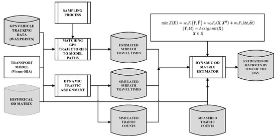
Figure 1.
Methodological diagram.
3. Direct Inclusion of ICT Measurements in the Model Formulation: An SPSA Approach to Solve the DODME Problem with Partial Path Travel Times
Since the relationship is not analytical and is induced from the DTA, and, at least in our case, the network loading of the DTA is done using a mesoscopic traffic simulation, the upper-level optimization problem has to be solved by resorting either to a derivative-free optimization method or a numerical approach that is based on a numerical approximation of the derivatives. Considering the references made in the introduction and our own experience [9], the approach chosen was the SPSA (stochastic perturbation stochastic approximation).
Although analytically founded, the SPSA (stochastic perturbation stochastic approximation), originally proposed by [28], can be considered heuristic in nature since it depends on parameters whose values cannot be calculated analytically. SPSA is an optimization method that estimates the direction of descent by calculating a stochastic gradient and evaluates the objective function only twice instead of times, as in the case of a finite-difference gradient approach, where M is the number of OD pairs times the number of considered periods. This is appropriate for cases where the objective function cannot be analytically expressed as a function of the parameters and when the evaluation is costly because it requires a simulation engine to produce the data that are involved in the evaluation. This is the case in the DODME problem, where a gradient approximation with only two dynamic traffic assignments is desirable because it is the most time-consuming step of the optimization, especially in the case of large networks.
Formally, a SPSA is a gradient optimization procedure that starts from an initial origin-to-destination (OD) matrix, usually a historical OD matrix, and the next point is computed using the first-order Taylor development:
where is the gradient that is calculated during the kth iteration from the current estimation of the OD matrix and is the step length along the gradient descent direction. SPSA (stochastic perturbation stochastic approximation) estimates the gradient since it cannot be calculated analytically, calculating it numerically as:
where is a random perturbation N-dimensional vector with , independent identically distributed random variables satisfying and . Note that only two evaluations are required. , which is a Bernoulli distribution with the probability for each outcome, is the usual perturbation used.
The spacing coefficient and the step size are decreasing sequences of positive real values that satisfy some regularity conditions to ensure the convergence of the method, as detailed in [28]. A detailed discussion on how the best values can be estimated and the possibility of auto-adaptive calculation approaches can be found in [6,9].
This paper implements a version following the recommendation of [28], which involves averaging a predefined number of independent estimations of the gradient of Equation (5) to contribute to a more stable and quicker convergence of the SPSA (stochastic perturbation stochastic approximation) method. Therefore, the gradient estimation is finally
where is calculated as in Equation (5). The objective function is formulated in this DODME, including travel times, as:
where the discrepancies between the estimated origin-to-destination (OD) matrix and the historical OD matrix , the measured link flows and the corresponding estimated flows , and the measured and estimated travel times are quadratic functions with weights , and that must be adjusted in order to adapt the magnitudes of each measure and to give more or less importance to each measure depending on its reliability. The indices and identify an origin and a destination, respectively, that belong to the set of all origin–destination pairs, the index r corresponds to the trip departure time interval; the index l identifies the link with a counting station in the subset of links with counting stations; t identifies the counting time interval; and the index identifies the subpath belonging to the set of the subpaths for periods in which the time horizon is split.
4. An Alternative Approach: The Hybrid SPSA (Stochastic Perturbation Stochastic Approximation)
In addition to the SPSA approach, a new one was developed and computationally tested by expanding and adapting a suggestion that was made by [11]. The optimization problem was the same as in Section 3 but the objective function was redefined as follows:
where is the assignment matrix that is estimated from the DTA [5,9], which is assumed to be constant on a neighborhood of the origin-to-destination (OD) matrix .
The idea behind this approach is to find the best approximation of the gradient by considering the analytical components of the objective function for which the analytical derivation is computable, where the non-analytical terms are:
where is calculated by using the SPSA (stochastic perturbation stochastic approximation) approach but the other terms are the formal partial derivatives of their analytical forms. This is the gradient used in this hybrid SPSA:
5. Indirectly Accounting for the ICT Measurements
Recent literature addresses how to include ICT measures into the DODME problem to reduce the underdetermination of the underlying problem. A two-step ordinary least squares (OLS) OD estimation model is proposed in [23], incorporating the output from a Bayesian path reconstruction model that was developed to cope with an insufficient coverage rate of ICT data from license plate recognition and estimates both the dynamic OD demand and assignment matrix without the need for any historical matrix. Finally, refs. [13,16] used the geopositioning data of probe vehicles from an ad hoc experiment that was designed by the authors to obtain an a priori dynamic origin-to-destination (OD) matrix and the reconstructed paths are included in the OD estimation process, and [17] used a data-analytics-based proprietary procedure to empirically estimate a dynamic assignment matrix.
The linearization of the relationship between traffic counts and OD flows is the approach of most analytical models that are used to solve DODME [9]. This can be achieved by using the proportion of the OD demand flows that pass through the count location at a certain link. In these terms, the dynamic assignment matrix is the result of the mapping and represents the proportion of the OD flow that departs from origin i in period r and goes to destination j that crosses link in period .
These analytical approaches to the DODME problem show that all of them rely on the availability of the assignment matrix for the various time intervals, which are calculated at the lower level of the bi-level problem using the dynamic traffic assignment at each time interval.
The availability of the GPS-generated data enabled us to assume that, after suitable data processing to find the empirical paths and the inference of path choice proportions, it was possible to estimate a dynamic assignment matrix that relied on the information regarding traffic conditions. Since it would play a similar role to that of the analytical assignment matrix that is obtained by a DTA, it would, if appropriately processed [19], estimate a reliable assignment matrix from the available commercial data.
The possibility of estimating an assignment matrix allows for reformulating the DODME by relating the estimated traffic counts with the OD flows using the estimated assignment matrix:
where is the estimated flow in link l in period t; is the flow departing origin i with destination j in time interval ; and is the estimated assignment matrix, which is the fraction of trips from origin i with destination j that depart from i in time interval r and reach link l at time t, as estimated from the GPS traces.
There are different approaches that are used to estimate the dynamic assignment matrix from the GPS traces. In [13], it is implicitly considered that this estimate is directly provided by a counting process, assuming that the analyst has complete control over the raw data collected, whereas in other cases when such control is not available and the access to the preprocessed data is provided by commercial companies, some drawbacks appear, which are derived from privacy conditions. Reference [17] assumes that access to very large data sets (i.e., at least 6 months) and an undisclosed proprietary data analytics application was available to generate the estimated assignment matrix. In [19], we proposed an indirect procedure that was based on the most reliable data supplied by commercial GPS providers, which involves the waypoints that usually take the form , where k denotes the trip identity; l is the ordered lth waypoint of trip k; ts is the time stamp; and lat and long are the geographic latitude and longitude, respectively. The approach studied in [19], in essence, proposed the following:
- A graph network model that is supplied either by transport planning software or by a GIS like OSM;
- A standard map matching that associates waypoints with the corresponding points in the links of the network, from which, the link travel times can be heuristically estimated;
- When using appropriate k-shortest paths, a suitable route choice set can be calculated;
- When considering the path overlapping factors, the reliable path proportion , which is the proportion of trips traveling from origin i to destination j leaving origin i at time r and using path k, can be calculated.
The assignment matrix can then be calculated using:
where is the link–path incidence matrix:
In Equation (11), the estimated assignment matrix is combined with the estimated origin-to-destination (OD) matrix to obtain the estimated link flows . In the bi-level optimization problem, the OD flows are always the variables that must be adjusted to minimize the objective function. However, from experience with analytical approaches [9], we observed in our experiments that OD flows may be substantially modified to fit traffic counts that imply high volumes to certain OD pairs, which is a drawback that can be overcome with a data-driven approach that aims to preserve the OD pattern that is included in the seed OD matrix.
The proposed formulation was inspired by gravity models, where it sets bi-dimensional constraints for rows and columns, as in the double-constrained models that are common for updating gravity distribution models [29]. Therefore, the origin-to-destination (OD) flow appearing in Equation (11) can be decoupled into independent scaling factors that are different for origins and destinations, expanding a seed matrix that, if the collected data are suitable, can be the observed OD matrix:
If are the link flows that are measured at the counting stations and is the dynamic assignment matrix that is estimated from GPS data, then data-driven DODME models can be formulated [17,19]. These modeling approaches do not need to resort to a dynamic traffic assignment to estimate the dynamic assignment matrix since it is estimated from GPS data. Reference [19] formulates the problem as the following nonlinear optimization problem whose variables are the scaling factors and :
An advantage of this formulation is the dimensionality reduction from to . Moreover, using the scaling factors as variables aims to preserve the structure of the seed origin-to-destination (OD) matrix, as gravity models do. On the other hand, in this formulation, the objective function is not quadratic; therefore, it requires appropriate optimization methods to solve it. In this study, our main concern was testing the quality of the results, not the development of an ad hoc algorithm. Therefore, to solve the minimization problem, the L-BFGS-B method [30] was chosen. It is a quasi-Newtonian method that is suited for constrained nonlinear problems with a high number of variables that efficiently reduces the memory requirements and the computational burden, especially when there is the risk of ill-conditioned Hessians, as could be the case due to the presumable flatness of the objective function. Moreover, the objective function that is given in Equation (14) is a quartic polynomial function with respect to the variables of the problem, which means that it is convex and a minimum is guaranteed.
6. Consideration on the Quality of the DODME Results
The quality of the results of the origin-to-destination (OD) estimation problem is usually established in terms of the convergence of the optimization algorithm that is used to solve the bi-level problem and the fitting of the simulated to the observed link flows. In addition, when a reliable historical OD matrix is available, a measure comparing the estimated OD X and the historical is added as a quality indicator. The typical measures that are used are based on classical vector matrices by considering both of the matrices as vectors of . However, refs. [4,9,31] proved that the measures that are defined using Euclidean (), Manhattan (), or other similar vector distances fail to capture the differences and similarities between the two matrices in many aspects, for example, the structure of the matrices. They present numerical examples where a reference OD matrix can be perturbed to generate two structurally different matrices that are indistinguishable in terms of these measures. This is a critical aspect to account for given that the underdetermination of the problem formulation means that many different OD matrices can generate the same observed link flow measurements; therefore, if they are structurally different, which is the most credible? On the other hand, proving that the optimization algorithm numerically converges only proves that it converges to a solution, but how good is that solution? If the complementary quality indicator is the R2 goodness of fit between the observed and the simulated link flows at the available counting stations in the subset of links , it may happen, as shown in [9], that the optimization algorithm behaves as a kind of meta-regression model that pulls from or pushes to the OD entries just to improve the fitting to traffic counts and travel times, ignoring the underlying reality of the physical transportation problem, where trips from origin i to destination j are a consequence of a socioeconomic reality that cannot increase or decrease the number of trips between this OD pair just for numerical needs and, thus, modify the underlying OD pattern.
In practical applications, if a reliable historical origin-to-destination (OD) matrix is available, the number of trips may be outdated for the structure of the matrix, but will still be relevant; therefore, it would be desirable that the structure of the estimated OD matrix be as close as possible to the structure of the historical matrix . A measure of similarity borrowed from image quality assessment to compare two different images is proposed in [4]. Reference [32] presents SSIM (structural similarity) for a matrix of pixels as a product of three different comparison components: luminance, contrast, and structure. Luminance corresponds to the intensity of illumination, which is the mean of the different pixels in a sub-matrix. Contrast is the root of the squared average between pixels once the luminance is removed, i.e., it is the standard deviation, and finally, the structure comparison is done by using the covariance between the two matrices. These three factors are first transformed with the aim to adjust them to the interval , where 1 means a perfect match and 0 means totally different. SSIM, therefore, is a similarity measure that is independent of the magnitude of the values in the matrix. The formula summarizing this explanation is below:
where luminance, contrast, and structure are respectively defined as:
where and are the means, standard deviations, and the covariance of the vectors and , respectively. and are stability constants to avoid numerical problems; these are typically set to . are weighting coefficients, which are typically set to 1 [32]. During the image comparison, the MSSIM is computed as the mean of the SSIM of all the sub-matrices of dimension N because pixel proximity is crucial in image pattern recognition. A variant of MSSIM is proposed in [15,18] including it in the objective function of the formulation of the mathematical model in Equation (3) after setting specific relationships between the measured and estimated travel times that are measured using ad hoc layouts of Bluetooth antennas, which are not reproducible when travel times are measured by other technologies, such as GPS.
Regarding the original problem, ref. [32] obtained the MSSIM by averaging the SSIM using sliding windows, which were submatrices of size Ns. When extrapolating the sliding windows to OD matrices, ref. [4] proposed reordering the origin-to-destination (OD) matrix by volume, both by rows and by columns, in order to obtain the MSSIM using the same sliding submatrices because the term S of the SSIM is highly sensitive to the order of the OD pairs. Another open question is the dimension of the submatrices Ns, which should be fixed, and it does affect the final measure. Reference [31] also reorders the OD pairs, but in this case, they proposed clustering them in greater regional areas. In the same article, they showed how the dimension of the submatrices affects the MSSIM measure; as such, this new proposal solves the problem of tuning Ns, which is fixed automatically by the dimension of these regional areas.
Here we proposed a more meaningful variant that is easier to apply in practice and considered the physical meaning of the origin-to-destination (OD) matrices. This variant consisted of calculating the averages of the SSIM according to rows and columns rather than submatrices, that is, by using rectangular sliding rules that correspond to either rows or columns in the OD matrix. One row in an OD matrix for a given period represents the distribution of trips that depart from a single origin zone while, analogously, one column is the distribution of trips arriving at a single destination zone. This, therefore, corresponds to a physical interpretation of mobility patterns in the underlying transport system. Thus, the SSIM will capture the similarity between these described distributions by considering the mean, variance, and structure of the departure and arrival distributions, all of which correspond to the structural property of the trip patterns that are described by the OD. Moreover, this proposal also fixes Ns to the number of origins and destinations in the network. Then, if the MSSIM is averaged over Ns sliding windows, a key question arises regarding whether all windows have the same weight or whether their role in the total demand requires that they have different weights. In the case of OD matrices, it is obvious that not all origins and destinations are equivalent in a transport network. Therefore, a weighted MSSIM, as in [33], prioritizes those origins and destinations with more impact on the network.
This proposed weighting average is defined as follows:
where and are the ith windows of X and , respectively, while the weight is given by:
In terms of the variance of the selected windows in the origin-to-destination (OD) matrices, these weighting factors correspond to the variance of the total generated trips from an origin (or total attracted trips to a destination) to all destinations (from all origins); thus, the weighting is increased as the origin is distributed to all destinations (or the destination attracts trips from origins) becomes more non-uniform. Moreover, these weights also take into account the magnitude of their contribution (implicitly in the variance value) so that the contribution of each origin or destination to the overall demand pattern is well balanced.
Under the assumption of the reliability of the historical OD matrix , at least concerning the structural information on the mobility patterns that it contains, in this study, we proposed to use the relative difference in the MSSIM calculation in Equation (17) between the estimated OD matrix X at iteration k and the historical OD matrix as stopping criterion. The stopping criterion is:
When no historical OD matrix is available, or the historical OD matrix is unreliable, a way of avoiding the fitting process distorting the structure could be to apply the alternative criterion:
This is based on the relative structural change of the estimated matrix after each step of the iterative process.
7. Synthetic Experimental Framework
In most papers that deal with DODME by adding richer ICT traffic measurements to the conventional link flow counts [13,16,17], the authors assume specific conditions for controlling the data collection processes, such as those proposed by [17,34,35]. These conditions for collecting the data ensure their quality and allow for making assumptions that form the basis of the approaches. This is not always possible with commercial data because the researcher has no access to it, the fleet size is very limited, or the only available data are supplied by commercial companies who prohibit access to the whole raw data set, which they pre-process, depending on their business model. Therefore, it is common to conduct simulation experiments that emulate reality, which is then mimicked by generating synthetic data. Reference [1] provides an experimental framework was widely used by researchers. However, they used specific microscopic simulation models and numerical software (i.e., MATLAB). This is why we propose a synthetic and agnostic software data generation process that fulfills the functional requirements and provides data that are indistinguishable from the actually measured data consisting of:
- A learning process that is supported by the analysis of a sample of GPS waypoints from an equipped fleet;
- Building a microscopic traffic simulation model of a traffic network that emulates the behavior of individual vehicles, including the class of equipped vehicles;
- Developing an APP to properly emulate the GPS data collection from the equipped vehicles (e.g., replicating the waypoint data collection policies).
Figure 2 depicts the conceptual diagram of the proposed methodology. To conduct the computational experiments that are reported in this paper, this methodological framework was implemented in PTV Vissim and PTV Visum, where the DTA used was the SBA implemented in Visum [36]. It was applied to a model of the city of Hillsboro, USA, consisting of 618 links and 58 zones. The simulation ran over a time horizon from 08:00 am to 09:00 am in three periods of 20 min; 120 days were generated in Vissim in order to obtain enough GPS trips with different random seeds and time latencies based on the learning process from the physical data. The full GPS data set contained 9.1 M waypoints, which is approx. 109 k trips. This data set was transformed to PrT paths in Visum using the GPX import tool and its map matching techniques to obtain the interpolated travel times at the link level from the sequence of waypoints.
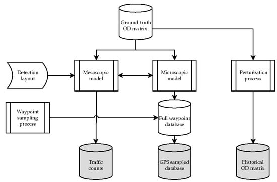
Figure 2.
Conceptual diagram of the synthetic data generation for computational testing.
Subpaths Extraction
A heuristic procedure that was used to obtain the “most used subpaths” from the GPS sample was designed. The implemented procedure was the following:
- From the list of paths in Visum, called PrTPaths, that were generated by the map-matching process and the links that they use, the heuristic started by selecting the most used link by paths. An example highlighted in purple is depicted in Figure 3.
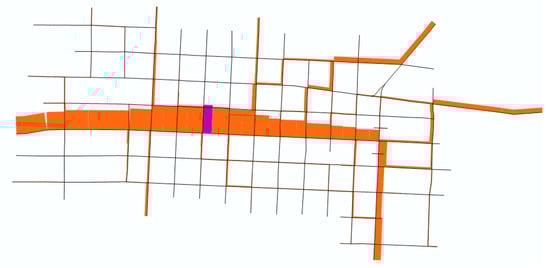 Figure 3. OD path flows that were intercepted by link .
 - Selecting all the paths that use the selected link, a search simultaneously found the forward and backward maximal subpaths.
- The procedure stopped when the number of paths that were used by link (subpath ) was reduced to a percent stop = 20% from the initial link . The percent stop was a design parameter.
- Once the subpath was selected, the links that formed this subpath were removed from the list of candidate links to define the most used paths. The list of paths and candidate links for step 1 was updated. The procedure returned to step 1.
- The iterative procedure was executed by also considering the departing period of each PrTPath to find subpaths for each period of the simulation and capture its dynamicity. It iterated until no more paths were found; in this case, 379 subpaths were found (127 on T1, 123 on T2, 129 on T3). The observed path travel times were calculated as the sum of their observed link travel times.
These subpaths with the observed travel time covered the entire network, as shown in Figure 4, and they were used by many GPS paths (158 on average), which allowed for confidence in their use and their observed travel time. The average length of these subpaths was 911 m. In this network, a subpath was considered if the number of links was greater than five.
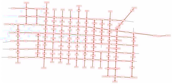
Figure 4.
Hillsboro network that was covered by the 450 subpaths.
8. Computational Results
The minimization problem that was used for the experiments is the one shown in Equation (21):
The three methods that were used in the computational experiments were:
- An SPSA (stochastic perturbation stochastic approximation) with travel times and the objective function defined in Equation (4);
- A hybrid SPSA with travel times and the objective function defined in Equation (5);
- A data-driven approach with the objective function defined in Equation (14).
Following the computational experience in [1], when the SPSA (stochastic perturbation stochastic approximation) is used, a constrained SPSA variant is applied in which the feasible set is determined by the bounding constraints, as shown in Equation (22), whose objective is to help to preserve the structural similarity:
The term of Equation (22) represents an acceptable relative change of the solution relative to the historical OD matrix, which serves as a reference, and is expected to be reliable based on the empirical background provided by the demand analysis practice. In these experiments, 0.2 was used based on common practices in traffic analysis applications.
A total of eight experiments were performed in order to see the effects of each of the proposed innovations. Three main factors were combined to generate the set of experiments:
- The term of the reference historical OD matrix on the objective function ( or );
- The term of travel times on the objective function ( or );
- The hybridization, or not, of the SPSA (stochastic perturbation stochastic approximation) gradient.
All the experiments used the matrix that was proposed for benchmarking purposes in MULTITUDE Cost action [1] as the historical OD matrix, normalizing the variables in the objective function. The weight was set to in order to equalize the importance of traffic counts and travel times.
Figure 5 summarizes the computational results in terms of the structural similarity index MSSIM and the total number of trips.
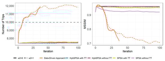
Figure 5.
Number of trips and the MSSIM evolution during the optimization procedure.
On the one hand, the addition of the term comparing the historical origin-to-destination (OD) matrix () and the addition of travel times to the problem allowed for an increase in the total number of trips to get closer to the ground truth , and the estimated OD matrices were more reliable from the structural point of view, namely, in the hybrid approach, which showed a more consistent behavior. It can be appreciated that in the case of the hybrid SPSA without travel times, the effect of adding the historical OD matrix () was negligible because the curves overlapped. This was because the optimization process was not stochastic anymore and the contribution of the term was not significant.
On the other hand, it was experimentally shown that the hybrid SPSA (stochastic perturbation stochastic approximation) gradient in Equation (6) outperformed the SPSA gradient. As expected, the analytical part of the gradient of the linearized objective function was a better approximation of the maximum descent direction. This effect was notably appreciated in the cases of . However, when , the effects of the hybrid SPSA vanished because of the SPSA-gradient-based part.
Figure 6 shows the simulated and real traffic measurements that were related to the objective function in the case of . Table 1 summarizes the adjustment and the MSSIM between the measurements.
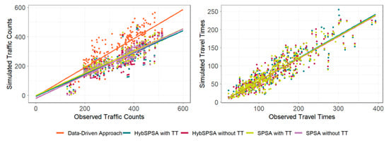
Figure 6.
Traffic count and travel time linear regressions when .

Table 1.
adjustments and MSSIM between measurements.
Regarding the traffic counts, the inclusion of the travel times in the objective function decreased the . On the other hand, the two variants of the SPSA (stochastic perturbation stochastic approximation) with travel times adjusted the paths travel times relative to the real measurements well, but the SPSA with travel times showed greater values.
In Figure 6, a remarkable group of outliers is shown for the traffic counts measurements. All these points belonged to the same detector in the outer limits of the study area and appeared for all methods, indicating that the traffic counts could not be satisfied without perturbing the global fit. A general trend can be highlighted: the SPSA (stochastic perturbation stochastic approximation) without travel times method had a greater because the estimation procedure behaved as a metamodel that modified the output matrix in such a way that traffic counts were forced. Nevertheless, as travel times were included, a compromise between the traffic counts and travel times had to be met and a joint enhancement required relaxing the traffic counts fit to obtain a global benefit in the estimation of the output matrix.
The obtained results when the historical matrix term was included in the objective function were generally beneficial in terms of the structural similarity and R2 for counts and travel times (if included). These results were consistent with the common practice that considered historical matrices as reliable reference matrices. Obsolete matrices that are available in some practical applications should not be included in the objective function for an origin-to-destination (OD) matrix adjustment.
In the left panel of Figure 7, the evolution of the MSSIM indicator, calculated as a comparative index relative to the historical matrix in one of the approaches (DDAF), is shown. Wide oscillations were present in the first few iterations; nevertheless, smooth behavior was found as the optimization progressed, indicating structural similarity pattern convergence to the historical matrix. In the right panel of Figure 7, even a weaker oscillation of the MSSIM indicator (Equation (20)) was obtained when comparing two consecutive iterations of the matrix estimates; in terms of structural similarity, this behavior indicated that the proposed DDAF formulation smoothly converged to the resulting matrix.
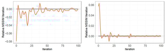
Figure 7.
Relative changes of the MSSIM according to Equations (19) and (20) for the data-driven results when . The performed band used .
9. Conclusions
The origin-to-destination (OD) estimation problem is an underdetermined problem that, depending on the used seed OD matrix, could lead to the resulting OD matrices fitting traffic counts but losing the OD trip pattern from available historical matrices. We focused on reducing such underdetermination using new ICT traffic measurements and improving the quality of the estimated matrices.
The knowledge that was acquired can be summarized in two ideas: first, the stochastic approaches that were based in SPSA (stochastic perturbation stochastic approximation) showed slow convergence and a high computation time. They failed to preserve the structural similarity of the resulting matrix compared with a reliable origin-to-destination (OD) historical matrix and they were incapable of increasing the total number of trips. As a benefit, they allowed for adding as many traffic measurements as desired into the objective function.
Second, analytical approaches rely on a dynamic assignment matrix estimation and they become extremely complex when they include additional traffic measurements to the traffic counts. In another work [19], we addressed the estimation of the dynamic assignment matrix from GPS data, and the DODME problem was reformulated, leading to a DDAF method. The quality of the estimated origin-to-destination (OD) matrices was better at preserving the structural similarity of the OD matrix relative to a reliable OD historical matrix, where the number of trips was increased/decreased when needed and fast convergence was obtained.
The main contribution of this article relied on the comparison of simulation optimization and the new analytical method using an experimental design that was based on synthetic data. The experimental framework allows for optionally adding information from GPS tracking to traffic count measures and a distance term to a reliable origin-to-destination (OD) historical matrix. Well-known goodness-of-fit indicators (, RMSE, and number of trips) and a revised proposal as a structural similarity index were collected for the SPSA (stochastic perturbation stochastic approximation) and DDAF approaches when the stopping criteria were modified.
The primary conclusion supports the use of a modified stopping criterion that was based on the variation of structural similarity that limited the number of iterations relative to classical stopping criteria. This new criterion was shown to provide remarkably good results in terms of structural similarity in the DDAF approach.
As a secondary conclusion, the DDAF approach that was proposed by the authors is the only method that has been shown to be capable of improving the total number of trips as needed. The number of trips of the estimated matrix has been rarely taken into account as a goodness-of-fit indicator. The best results were obtained for the DDAF approach when a distance term to a reliable historical origin-to-destination (OD) was considered.
Lastly, but not least, adding a distance term to a reliable origin-to-destination (OD) historical matrix in the SPSA studied approaches and travel time data that were derived from GPS traces were shown to benefit the quality of the estimated OD matrix, although never reaching the remarkable results obtained with the DDAF approach. The results for the SPSA (stochastic perturbation stochastic approximation) approaches indicated an excellent fit to traffic counts and travel times at the expense of structural similarity and slow progress on the number of trips fitting to the ground truth value.
Author Contributions
Conceptualization, X.R.-R., L.M. and J.B.; methodology, X.R.-R., L.M. and J.B.; software, X.R.-R., L.M. and J.B.; validation, X.R.-R., L.M. and J.B.; formal analysis, X.R.-R., L.M. and J.B.; investigation, X.R.-R., L.M. and J.B.; resources, X.R.-R., L.M. and J.B.; data curation, X.R.-R., L.M. and J.B.; writing—original draft preparation, X.R.-R., L.M. and J.B.; writing—review and editing, X.R.-R., L.M. and J.B.; visualization, X.R.-R., L.M. and J.B.; supervision, X.R.-R., L.M. and J.B.; project administration, X.R.-R., L.M. and J.B.; funding acquisition, X.R.-R., L.M. and J.B. All authors have read and agreed to the published version of the manuscript.
Funding
This research was funded by the TRA2016-76914-C3-1-P Spanish R+D Programs, the Secretaria d’Universitats-i-Recerca-Generalitat de Catalunya- 2017-SGR- 1749 and Industrial Ph.D. Program 2017 DI 041, and the company PTV Group, based in Karlsruhe, Germany.
Institutional Review Board Statement
Not applicable.
Informed Consent Statement
Not applicable.
Conflicts of Interest
The authors declare no conflict of interest.
References
- Antoniou, C.; Barcelo, J.; Breen, M.; Bullejos, M.; Casas, J.; Cipriani, E.; Ciuffo, B.; Djukic, T.; Hoogendoorn, S.; Marzano, V.; et al. Towards a generic benchmarking platform for origin-destination flows estimation/updating algorithms: Design, demonstration and validation. Transp. Res. Part C Emerg. Technol. 2016, 66, 79–98. [Google Scholar] [CrossRef]
- Antoniou, C.; Azevedo, C.L.; Lu, L.; Pereira, F.C.; Ben-Akiva, M. W–SPSA in Practice: Approximation of Weight Matrices and Calibration of Traffic Simulation Models. Transp. Res. Procedia 2015, 7, 233–253. [Google Scholar] [CrossRef] [Green Version]
- Cantelmo, G.; Cipriani, E.; Gemma, A.; Nigro, M. An Adaptive Bi-Level Gradient Procedure for the Estimation of Dynamic Traffic Demand. IEEE Trans. Intell. Transp. Syst. 2014, 15, 1348–1361. [Google Scholar] [CrossRef]
- Djukic, T. Dynamic OD Demand Estimation and Prediction for Dynamic Traffic Management; Delft University of Technology: Mekelweg, The Netherlands, 2014. [Google Scholar] [CrossRef]
- Frederix, R.; Viti, F.; Tampère, C. Dynamic origin-destination estimation in congested networks: Theoretical findings and implications in practice. Transp. A Transp. Sci. 2013, 9, 494–513. [Google Scholar] [CrossRef]
- Kostic, B.; Gentile, G.; Antoniou, C. Techniques for improving the effectiveness of the SPSA algorithm in dynamic demand calibration. In Proceedings of the 2017 5th IEEE International Conference on Models and Technologies for Intelligent Transportation Systems (MT-ITS), New York, NY, USA, 26–28 June 2017; pp. 368–373. [Google Scholar]
- Osorio, C. Dynamic origin-destination matrix calibration for large-scale network simulators. Transp. Res. Part C Emerg. Technol. 2019, 98, 186–206. [Google Scholar] [CrossRef]
- Qurashi, M.; Ma, T.; Chaniotakis, E.; Antoniou, C. PC–SPSA: Employing Dimensionality Reduction to Limit SPSA Search Noise in DTA Model Calibration. IEEE Trans. Intell. Transp. Syst. 2019, 21, 1635–1645. [Google Scholar] [CrossRef]
- Ros-Roca, X.; Montero, L.; Barceló, J. Investigating the quality of Spiess-like and SPSA approaches for dynamic OD matrix estimation. Transp. A Transp. Sci. 2021, 17, 235–257. [Google Scholar] [CrossRef]
- Toledo, T.; Kolechkina, T. Estimation of Dynamic Origin–Destination Matrices Using Linear Assignment Matrix Approximations. IEEE Trans. Intell. Transp. Syst. 2012, 14, 618–626. [Google Scholar] [CrossRef]
- Tympakianaki, A.; Koutsopoulos, H.N.; Jenelius, E. Robust SPSA algorithms for dynamic OD matrix estimation. Procedia Comput. Sci. 2018, 130, 57–64. [Google Scholar] [CrossRef]
- Barceló, J.; Montero, L.; Bullejos, M.; Serch, O.; Carmona, C. A Kalman Filter Approach for Exploiting Bluetooth Traffic Data When Estimating Time-Dependent OD Matrices. J. Intell. Transp. Syst. 2012, 17, 123–141. [Google Scholar] [CrossRef]
- Yang, X.; Lu, Y.; Hao, W. Origin-Destination Estimation Using Probe Vehicle Trajectory and Link Counts. J. Adv. Transp. 2017, 2017, 4341532. [Google Scholar] [CrossRef]
- Carrese, S.; Cipriani, E.; Mannini, L.; Nigro, M. Dynamic demand estimation and prediction for traffic urban networks adopting new data sources. Transp. Res. Part C Emerg. Technol. 2017, 81, 83–98. [Google Scholar] [CrossRef]
- Behara, K.N.S. Origin-Destination Matrix Estimation Using Big Traffic Data: A Structural Perspective. Ph.D. Thesis, School of Civil Engineering and Built Environment Science and Engineering Faculty Queensland University of Technology, Brisbane, Australia, 2019. [Google Scholar]
- Krishnakumari, P.; van Lint, H.; Djukic, T.; Cats, O. A data driven method for OD matrix estimation. Transp. Res. Part C Emerg. Technol. 2020, 113, 38–56. [Google Scholar] [CrossRef] [Green Version]
- Mitra, A.; Attanasi, A.; Meschini, L.; Gentile, G. Methodology for O-D matrix estimation using the revealed paths of floating car data on large-scale networks. IET Intell. Transp. Syst. 2020, 14, 1704–1711. [Google Scholar] [CrossRef]
- Behara, K.N.S.; Bhaskar, A.; Chung, E. A Novel Methodology to Assimilate Sub-Path Flows in Bi-Level OD Matrix Estimation Process. IEEE Trans. Intell. Transp. Syst. 2020, 22, 6931–6941. [Google Scholar] [CrossRef]
- Ros-Roca, X. Dynamic OD Matrix Estimation Exploiting ICT Traffic Measurements; Universitat Politècnica de Catalunya: Barcelona, Spain, 2021. [Google Scholar]
- Spall, J.C. An Overview of the Simultaneous Perturbation Method for Efficient Optimization. Johns Hopkins Tech. Dig. 1998, 19, 482–492. [Google Scholar]
- Osorio, C.; Chong, L. A Computationally Efficient Simulation-Based Optimization Algorithm for Large-Scale Urban Transportation Problems. Transp. Sci. 2015, 49, 623–636. [Google Scholar] [CrossRef]
- Bullejos, M.; Barceló, J.; Montero, L. A DUE Based Bilevel Optimization Approach for the Estimation of Time Sliced OD Matrices. In Proceedings of the 4th International Symposium of Transport Simulation 2014 (ISTS’14), Ajaccio, France, 1–4 June 2014. [Google Scholar]
- Mo, B.; Li, R.; Dai, J. Estimating dynamic origin–destination demand: A hybrid framework using license plate recognition data. Comput. Civ. Infrastruct. Eng. 2020, 35, 734–752. [Google Scholar] [CrossRef]
- Salari, M.; Kattan, L.; Lam, W.H.; Esfeh, M.A.; Fu, H. Modeling the effect of sensor failure on the location of counting sensors for origin-destination (OD) estimation. Transp. Res. Part C Emerg. Technol. 2021, 132, 103367. [Google Scholar] [CrossRef]
- Yu, H.; Zhu, S.; Yang, J.; Guo, Y.; Tang, T. A Bayesian Method for Dynamic Origin-Destination Demand Estimation Syn-thesizing Multiple Sources of Data. Sensors 2021, 21, 4971. [Google Scholar] [CrossRef]
- Tang, K.; Cao, Y.; Chen, C.; Yao, J.; Tan, C.; Sun, J. Dynamic origin-destination flow estimation using automatic vehicle identification data: A 3D convolutional neural network approach. Comput. Civ. Infrastruct. Eng. 2021, 36, 30–46. [Google Scholar] [CrossRef]
- Barceló, J.; Gilliéron, F.; Linares, M.P.; Serch, O.; Montero, L. Exploring Link Covering and Node Covering Formulations of Detection Layout Problem. Transp. Res. Rec. J. Transp. Res. Board 2012, 2308, 17–26. [Google Scholar] [CrossRef] [Green Version]
- Spall, J.C. Multivariate stochastic approximation using a simultaneous perturbation gradient approximation. IEEE Trans. Autom. Control. 1992, 37, 332–341. [Google Scholar] [CrossRef] [Green Version]
- Ortúzar, J.D.D.; Willumsen, L.G. Modelling Transport; John Wiley & Sons, Inc.: Hoboken, NJ, USA, 2011. [Google Scholar] [CrossRef]
- Morales, J.L.; Nocedal, J. Remark on “algorithm 778: L-BFGS-B: Fortran subroutines for large-scale bound constrained optimization”. ACM Trans. Math. Softw. 2011, 38, 1–4. [Google Scholar] [CrossRef]
- Behara, K.N.S.; Bhaskar, A.; Chung, E. Classification of Typical Bluetooth OD Matrices Based on Structural Similarity of Travel Patterns: Case Study on Brisbane City. In Proceedings of the Transportation Research Board 97th Annual Meeting, Washington, DC, USA, 7–11 January 2018. [Google Scholar]
- Wang, Z.; Bovik, A.C.; Sheikh, H.R.; Simoncelli, E.P. Image Quality Assessment: From Error Visibility to Structural Similarity. IEEE Trans. Image Process. 2004, 13, 600–612. [Google Scholar] [CrossRef] [PubMed] [Green Version]
- Wang, Z.; Simoncelli, E.P. Maximum differentiation (MAD) competition: A methodology for comparing computational models of perceptual quantities. J. Vis. 2008, 8, 8. [Google Scholar] [CrossRef] [PubMed] [Green Version]
- Lopez, C.; Krishnakumari, P.; Leclercq, L.; Chiabaut, N.; van Lint, H. Spatiotemporal Partitioning of Transportation Net-work Using Travel Time Data. Transp. Res. Rec. J. Transp. Res. Board 2017, 2623, 98–107. [Google Scholar] [CrossRef] [Green Version]
- Lopez, C.; Leclercq, L.; Krishnakumari, P.; Chiabaut, N.; Van Lint, H. Revealing the day-to-day regularity of urban congestion patterns with 3D speed maps. Sci. Rep. 2017, 7, 1–11. [Google Scholar] [CrossRef]
- PTV AG. PTV Visum-User’s Manual; PTV AG: Karlsruhe, Germany, 2020. [Google Scholar]
Publisher’s Note: MDPI stays neutral with regard to jurisdictional claims in published maps and institutional affiliations. |
© 2021 by the authors. Licensee MDPI, Basel, Switzerland. This article is an open access article distributed under the terms and conditions of the Creative Commons Attribution (CC BY) license (https://creativecommons.org/licenses/by/4.0/).