Abstract
The interaction between subway tunnels is investigated by using a 2D analytic model of a twin tunnels system embedded in a homogenous half-space. The closed-form analytical solution for tunnel displacement response is derived through the wave function expansion method and the mirror method, and the correctness of the solution is verified through residuals convergence and comparison with the published results. The analysis focuses on the effects of tunnel relative stiffness on tunnel–soil–tunnel interaction. Tunnel relative stiffness has a great influence on tunnel displacement response. For small tunnel relative stiffness, tunnel displacement amplitude can be enlarged by 3.3 times that of single rigid tunnel model. The response of the tunnel–soil–tunnel interaction system depends not only on the distances between tunnels but also on the frequency of the incident wave and the incident angle. The strength of the interaction between the tunnels is highly related to the tunnel spacing distance. The smaller the distance between tunnels, the stronger the interaction between them. When the distance between tunnels reaches s/a = 20, the interaction between tunnels can be ignored. It is worth pointing out that the seismic design of underground tunnels should consider the interaction between tunnels when the tunnel distance is small.
1. Introduction
An underground tunnel is a shallow-buried structure located under the surface of an infinite half-space. Under the action of seismic excitation, it will generate dynamic interaction with the surrounding soil (known as soil–structure interaction, SSI). The methods for solving SSI problems can be roughly divided into two categories: analytical methods and numerical methods.
The analytical method mainly refers to the wave function expansion method, which mainly studies regular shape models embedded in a uniform half-space. Although the analytical method is only suitable for relatively simple and regular models, it has an advantage over the numerical method in revealing the essence of the problem. Therefore, enriching the analytical solution library is the goal that scholars have been pursuing. Pao and Mow [1] pioneered the application of the wave function expansion method of electromagnetic waves to the problem of seismic wave scattering and presented the out-of-plane dynamic analytical solution of a single buried tunnel in the whole space. Then, scholars further solved the analytical solutions of the dynamic response of a single tunnel embedded in an isotropic half-space, respectively excited by plane SH-wave, P-wave, and SV-wave [2,3,4,5,6].
Numerical methods include finite difference method, finite element method, and boundary element method. The numerical method is suitable for arbitrary-shaped tunnels and various site conditions and is more suitable for practical engineering problems. Fang et al. [7] showed the tunnel’s response by considering the nonlinear soil conditions. Wong et al. [8] studied the dynamic displacement and stress concentration of an arched tunnel. They found that the dynamic amplifications of the displacements and stresses induced in the tunnel depend crucially on the properties of the surrounding soil, the depth of embedment, and the frequency of the incident simple harmonic disturbance. Luco et al. [9,10] investigated the three-dimensional dynamic response of an embedded tunnel in a horizontally layered half-space under incident body waves. They extended the comparisons with previous two- and three-dimensional results for the case of a shell embedded in a uniform half-space, and some new numerical results for a shell embedded in a multilayered half-space are presented in a companion paper. Liu et al. [11] presented an analytic solution for the model of a circular lined underground tunnel in elastic half-space excited by in-plane waves, based on the method of complex functions introduced in [12]. The key idea to treat the boundary condition on the ground surface is to find a suitable conformal mapping that transforms the semi-infinite domain of the elastic half-space into a finite circular region, so the original flat half-space surface becomes a closed circle in the image plane which enables the parametrization using azimuthal variable. The advantage of conformal transformation is that some more complicated situations can be considered. Conformal transformation can transform irregularly shaped cross-sections into, for example, circular cross-sections through mathematical transformation, so that the original problem can be solved. The disadvantage of conformal transformation is that the mathematical derivation becomes more complicated. Recently, Parvanova et al. [13] studied the influence of local topography on tunnel dynamic response.
However, all the above studies on soil–tunnel interaction are focused on a single tunnel. Thus, this paper aims to investigate the dynamic interaction between twin flexible tunnels by using the wave function expansion method. The work in this article is an extension of Fu’s research on the seismic response analysis of a single rigid tunnel model [6]. The problem studied in this paper involves the seismic interaction between multiple underground structures, which is currently termed as structure–soil–structure interaction (SSSI) [14,15,16,17,18,19]. At present, the research of SSSI focuses on the interaction between multiple aboveground structures [20,21,22,23,24,25,26,27,28,29,30,31], and the research on the interaction between multiple underground structures have not been reported.
This paper notes that existing SSSI studies lack analytical solutions for the interaction of multiple underground structures, and it proposes a two-dimensional (2D) analytical model of the interaction between two tunnels. This model consists of two 2D infinite long flexible tunnels embedded in a homogenous half-space, subjected to incident SH-wave. The closed-form analytical solution of the twin tunnels interaction system response is obtained. The analytical solution is further used to reveal the interaction mechanism of the twin flexible tunnels system. The research can provide theoretical guidance and reference for seismic design of underground engineering, such as subway tunnels.
In the next section, the methodology is presented, followed by the verification through residuals convergence and comparison with the published results of the single rigid tunnel model [6]. Then, the results in the frequency domain are presented and the anti-plane tunnel responses are discussed. Finally, the main findings and the conclusions are summarized.
2. Methodology
2.1. Analytical Model
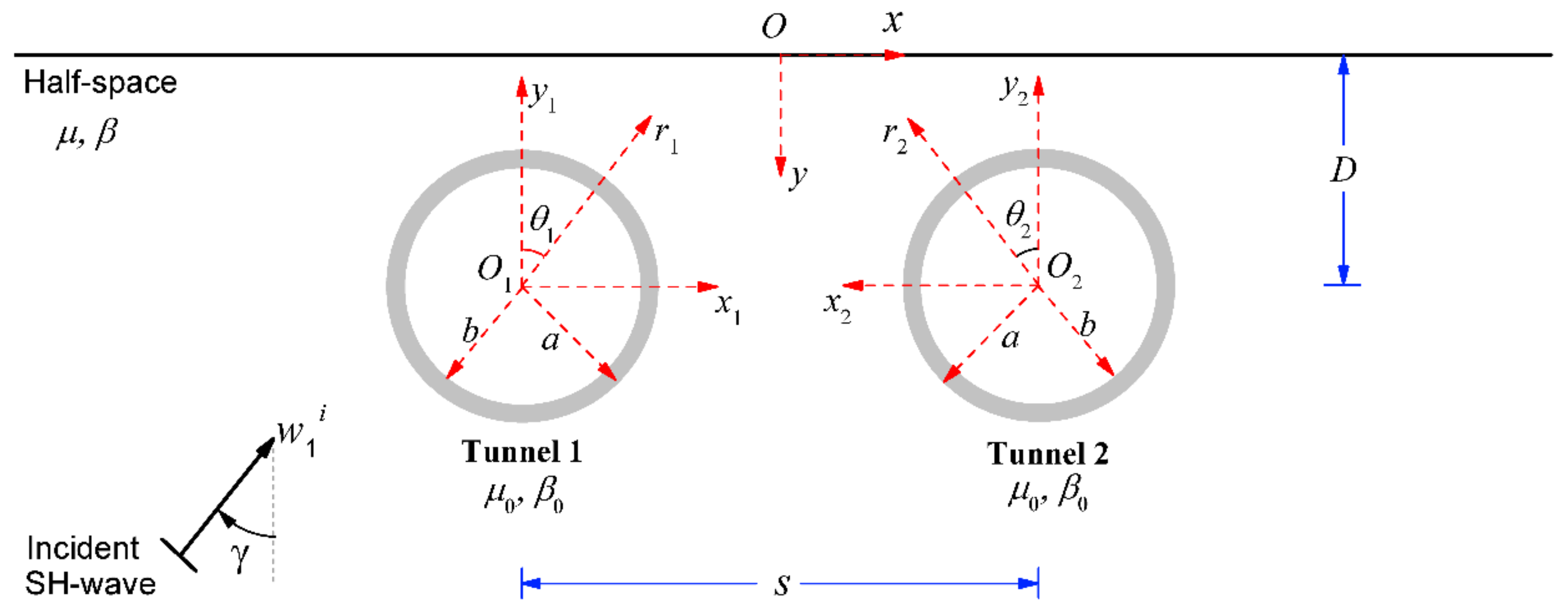
The dynamic tunnel–soil–tunnel interaction model, as shown in Figure 1, consists of twin flexible tunnels, infinitely long in the z-direction, embedded in a half-space. The z-axis of the rectangular coordinate system is perpendicular to the paper (points to the reader). The twin tunnels are circular with the centers at points of o1 and o2, and the outer radius and inner radius are a and b (b = 0.9a), respectively. With the points of o1 and o2 as the origin, there are two sets of coordinate systems. The rectangular coordinates and the corresponding cylindrical coordinates are drawn. The half-space and the two tunnels are assumed to be linearly elastic, uniform, and isotropic, and the boundary between the tunnel and the half-space is assumed to be tightly connected. The half-space is marked with shear wave velocity β, mass density ρ, and shear modulus μ. The tunnels are marked with shear wave velocity β0, mass density ρ0, and shear modulus μ0. The distance between the center o1 and o2 is s. The burial depth of the tunnels is D. An excitation is an incident plane SH-wave with circular frequency ω, incidence angle γ measured from the vertical z-axis, and unit amplitude. To reduce the complexity of the problem and obtain the analytical solution to the problem, the influence of underground water is ignored.
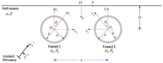
Figure 1.
The analytical model of dynamic tunnel-soil-tunnel interaction subjected to out-of-plane SH-wave.
2.2. Governing Equations and Boundary Conditions
The incident SH-wave motion in the half-space along the z-axis direction can be written in the local coordinate system (x1-y1-z1) as
where i is the imaginary unit and ω is the circular frequency of the incident wave.
The reflected wave will be generated when the incident wave propagates to the ground surface, and the scattered wave will be generated when it encounters the tunnels. Then, the total wavefield in the half-space is the superposition of incident wave, reflected wave, and scattered wave, all of which must satisfy the 2D wave equation.
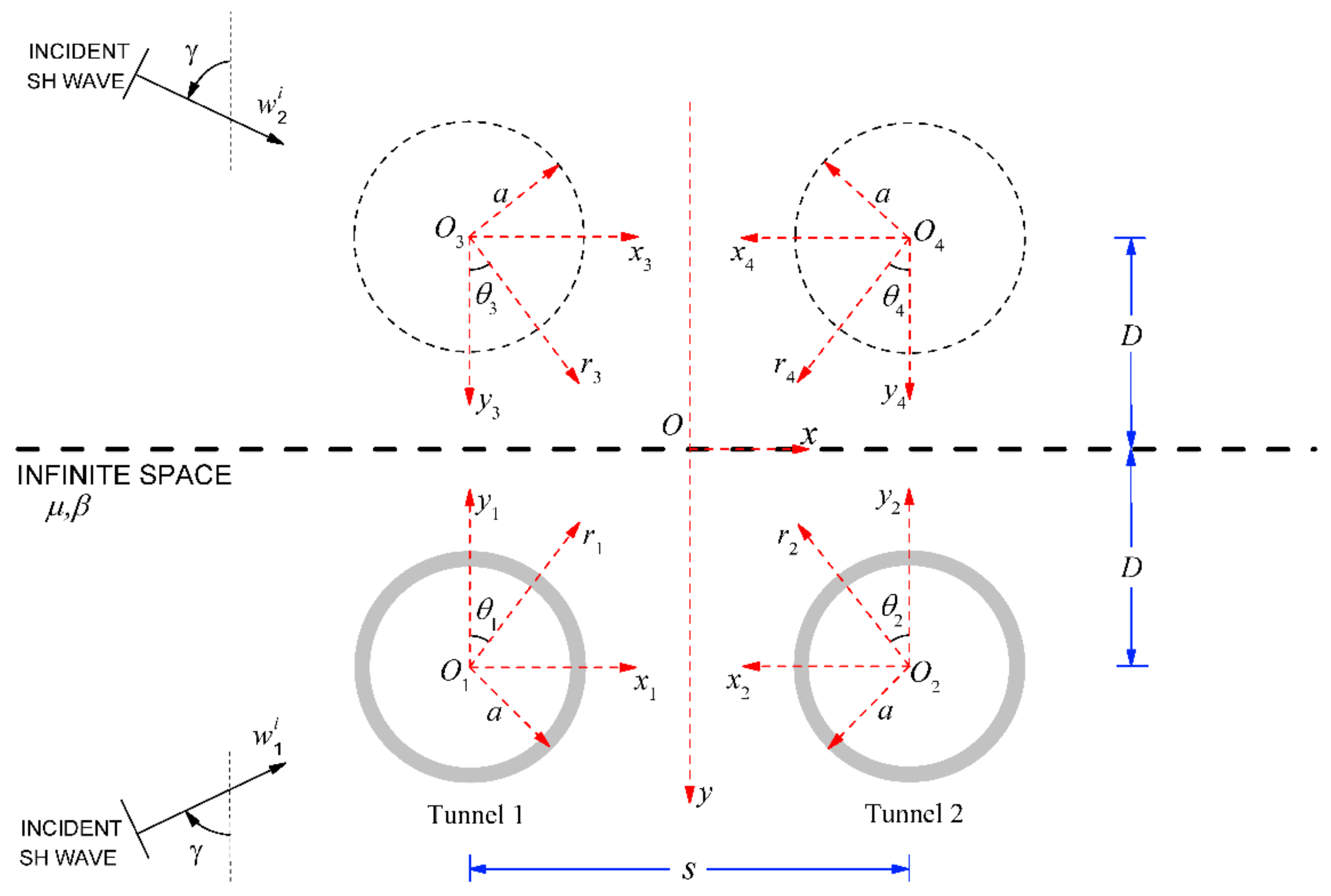
To satisfy the zero-stress boundary condition of the half-space surface, the mirror image method [32] is used to solve the problem. As shown in Figure 2, assuming that there is another incident wave source and two tunnels with an outer diameter, a, in the half-space with the surface as its axis of symmetry, the incident wave is
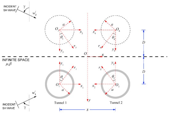
Figure 2.
Twin tunnels and their images.
The scattered wavefield corresponding to different tunnels can be expressed as
Here, is the Hankel function of the second kind with argument x and order m. The time factor exp(iωt) in Equations (1) and (3) is omitted in the subsequent formulas in this article. In the physical sense, they all represent cylindrical waves propagating outward from their respective centers, oi, satisfying wave Equation (2) and Sommerfeld radiation conditions. From the symmetry of the mirror method, it can be obtained that A1,m = A3,m, B1,m = B3,m, A2,m = A4,m, and B2,m = B4,m.
The wavefield in the flexible tunnels is
where k0 = ω/β0, and is the Hankel function of the first kind with argument x and order m.
All the wave motions must satisfy the boundary conditions given by
Since the wave functions and boundary conditions are represented in different coordinate systems, the coordinate transformation is required. With the help of Graf’s addition theorem [33,34] of the oblique coordinate system, coordinate transformation can be carried out between any two coordinates, and the details will not be described again.
2.3. Solutions to the Problem
Inserting Equation (4) into Equation (8), it can be obtained as
By using Equation (12) in Equation (4), Equation (4) can be rewritten as
Similarly, it can be obtained from Equation (11) as
where
For solving the response of tunnel 1, the incident wave should be transformed into the coordinate (r1, θ1). Then, the incident waves and can be expressed as
Similarly, all the scattered wavefields should also be transformed into the coordinate (r1, θ1) as
Similarly, for solving the response of tunnel 2, all the wave fields must be transformed into the coordinate (r2, θ2). It can be obtained as
Inserting Equations (30)–(34) and into Equations (9) and (10), it can be obtained as
Equations (22), (23), (35), and (36) constitute an infinite algebraic system of equations. Though setting the truncated number N, the four sets of unknown coefficients A1,m, B1,m, A2,m, and B2,m can be obtained by solving Equations (22), (23), (35), and (36) together. The analytical solution of the problem can be obtained by substituting the coefficients into the corresponding wave fields.
3. Solution Verification
The dimensionless frequency η, which is expressed in terms of the tunnel radius a, and the wave velocity β, is defined as [35]
where 2a is the tunnel diameter and λ is the wavelength of the shear waves in the half-space.
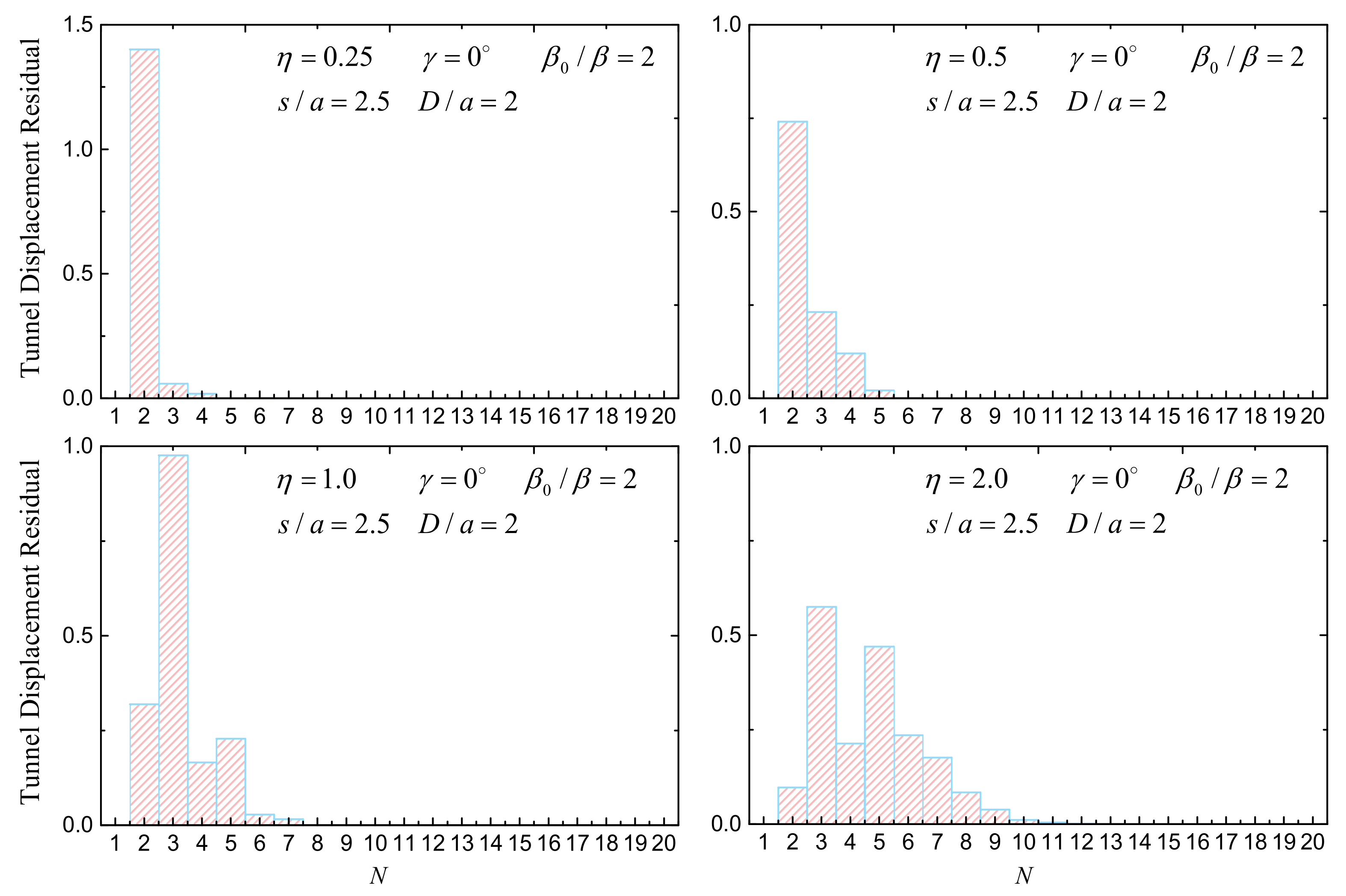
Figure 3 shows the convergence of tunnel displacement residual under four different dimensionless frequencies, η = 0.25, 0.5, 1.0, and 2.0, when s/a = 2.5, tunnel buried depth D/a = 2, and incident angle γ = 0°. For different incident wave frequencies, with the increase of truncation terms N, the error gradually approaches zero, which proves that the series solution in this paper can obtain a result that meets the accuracy.
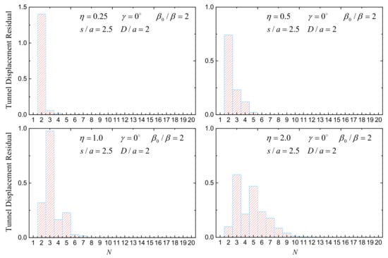
Figure 3.
Tunnel displacement residuals convergence.
4. Results and Analysis
4.1. Model Parameters
Figure 4, Figure 5 and Figure 6 show the effect of tunnel stiffness on tunnel responses. In comparison, the corresponding response of the single rigid tunnel model [6] is also plotted in each sub-figure. The parameters are as follows. The shear-velocity contrast between the tunnel and the half-space (we call it “tunnel relative stiffness”) β0/β = 2, 5, 10, and 100. The parameters for tunnel depth are D/a = 2 and tunnel distance s/a = 5, 10, and 20. The wave incident angle γ = 0° (vertical incident), 30°, 60°, and 90° (horizontal incident). The dimensionless frequency of incident SH-wave η = 0.25, 0.5, 1.0, and 2.0.
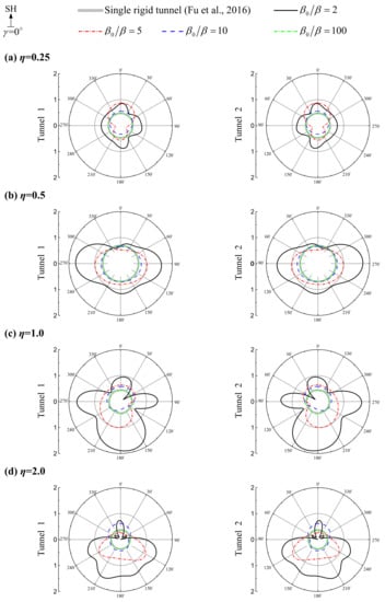
Figure 4.
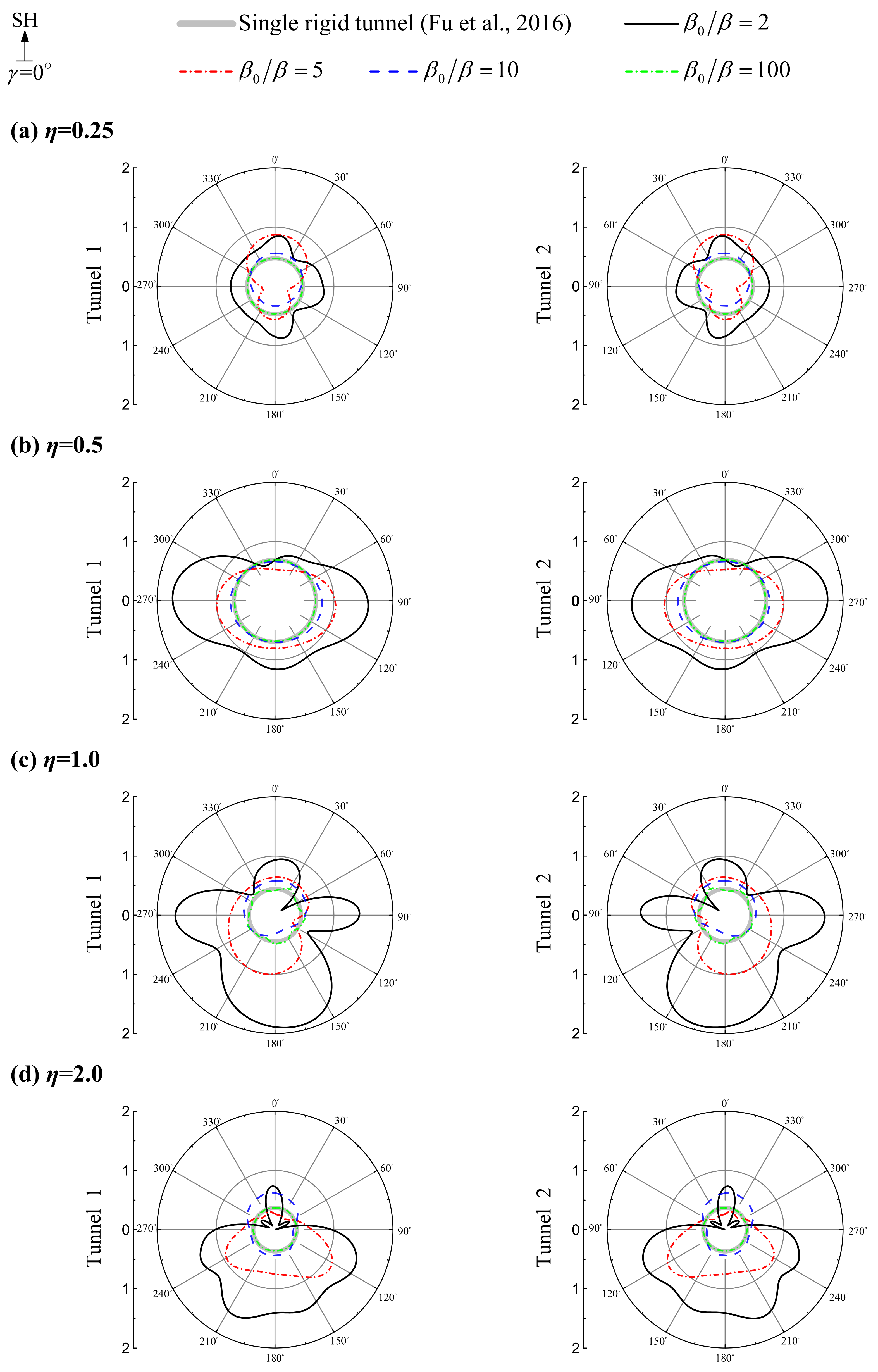
Typical spectral amplification of the tunnel displacement responses under different tunnel relative stiffness (β0/β) and dimensionless frequency (η) of the incident wave. Tunnel burial depth D/a = 2, tunnel distance s/a = 5, incident angle γ = 0° (vertical incident). Left column: tunnel 1; right column: tunnel 2. Parts (a–d) correspond to the dimensionless frequency η = 0.25, 0.5, 1.0, and 2.0, respectively.
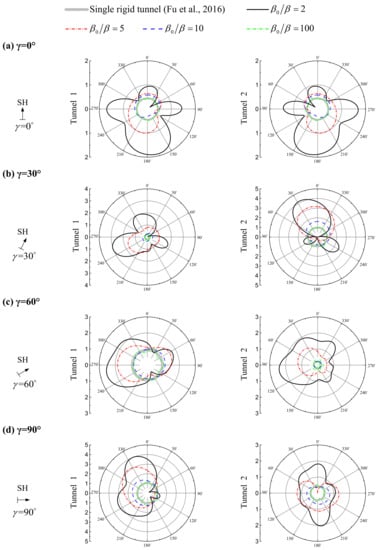
Figure 5.
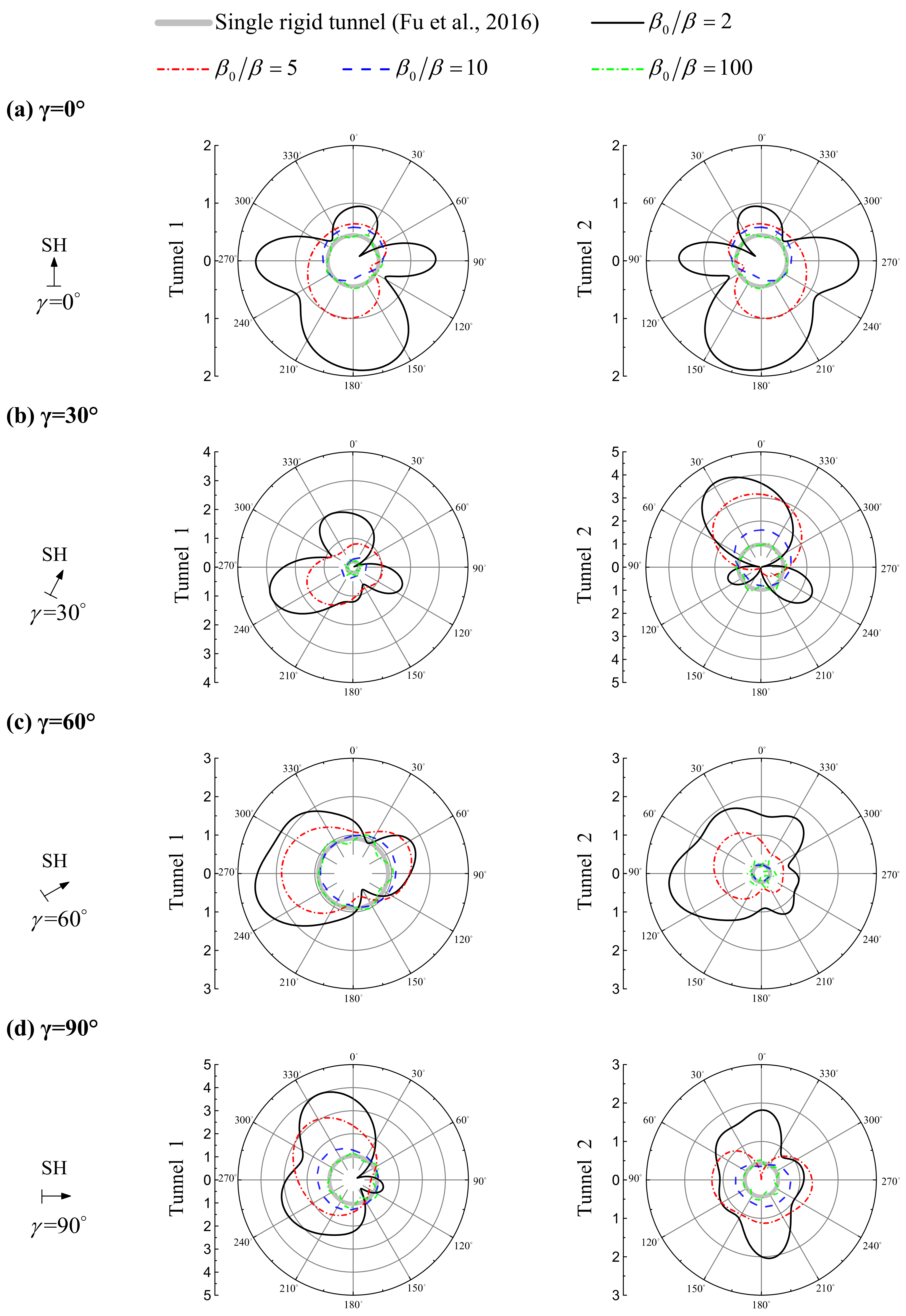
Typical spectral amplification of the tunnel displacement responses under different incident angles (γ). Tunnel burial depth D/a = 2, tunnel distance s/a = 5, dimensionless frequency η = 1.0. Left column: tunnel 1; right column: tunnel 2. Parts (a–d) correspond to the incident angle γ = 0° (vertical incident), 30°, 60°, and 90° (horizontal incident), respectively.
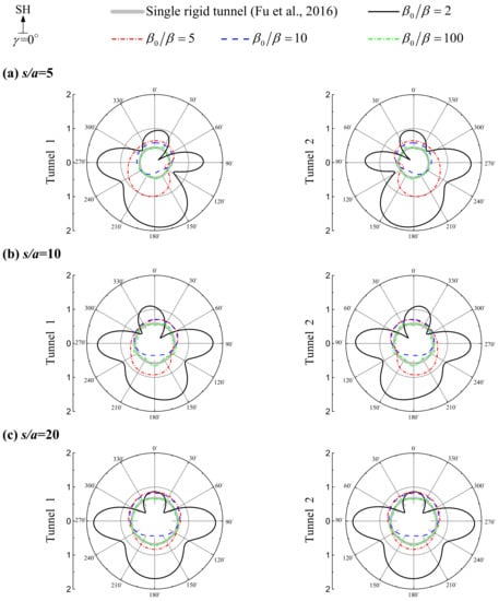
Figure 6.
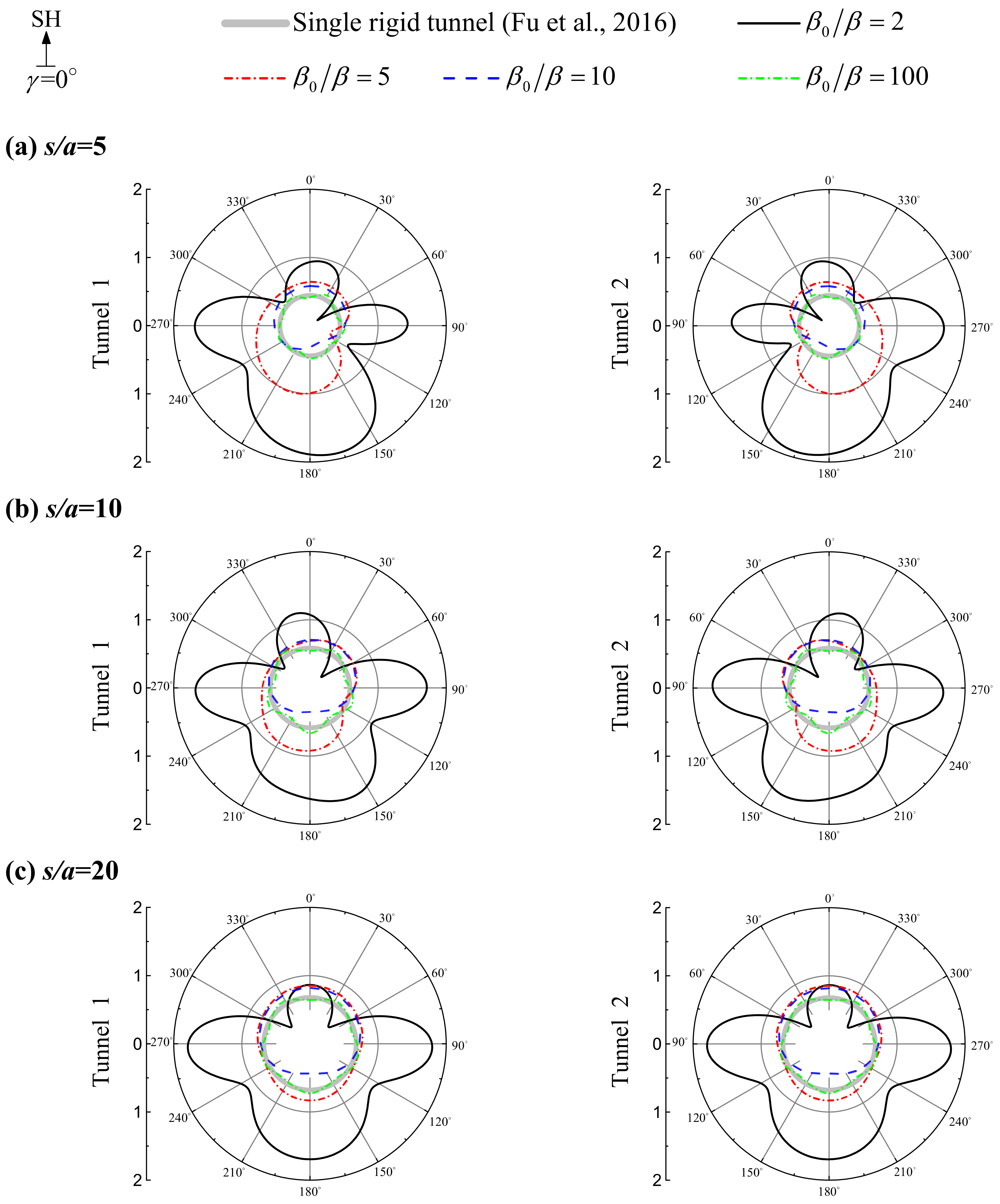
Typical spectral amplification of the tunnel displacement responses under different tunnel distance (s/a). Tunnel burial depth D/a = 2, dimensionless frequency η = 1.0, incident angle γ = 0° (vertical incident). Left column: tunnel 1; right column: tunnel 2. Parts (a–c) correspond to the tunnel distance s/a = 5, 10, and 20, respectively.
The analysis is arranged as follows. In Section 4.1, the model parameters are introduced. In Section 4.2, the influence of the tunnel relative stiffness (β0/β) on the two tunnels’ responses is investigated. For excluding the interference of other factors, only the results of the vertical incident (γ = 0°) are demonstrated. In Section 4.3, we further analyze the influence of the wave incident angle on tunnel response. In Section 4.4, the effects of the dimensionless distance between the twin tunnels (s/a) are discussed.
What needs to be pointed out is that, in this section, we only discuss the results that correspond to the tunnel buried depth D/a = 2. This is because the influence of the tunnel buried depth on the tunnel dynamic response has been reported in [6]. The conclusion in [6] shows that the shallower the tunnel buried depth (that is, the closer to the ground free surface), the greater the influence of the ground free surface and the stronger the interaction between the two tunnels. For deeper tunnels, the influence of the free surface is insignificant. In view of this, combining with some actual tunnel engineering data, we finally took the buried depth of the tunnel as D/a = 2 in this section, which is equivalent to studying the strongest interaction between the two tunnels.
4.2. Influence of Tunnel Stiffness on Tunnel Responses
Figure 4 shows the influence of tunnel relative stiffness (β0/β) on the response of the twin tunnel system by taking the results of the vertical incident angle γ = 0° and the tunnel spacing distance s/a = 5 as an example. As Figure 4 shows, for vertical incident angle (γ = 0°), when the tunnel has certain stiffness (β0/β = 2, 5, and 10), the displacement amplitudes of tunnel 1 and tunnel 2 are the same and are all larger than that of the rigid single tunnel [6]. For different dimensionless frequencies, with tunnel relative stiffness (β0/β) increases, the displacement amplitudes of tunnel 1 and tunnel 2 are decreasing and approach that of the rigid single tunnel [6]. For example, for η = 1.0, the displacement amplitudes of tunnel 1 that respectively correspond to tunnel relative stiffness β0/β = 2, 5, 10, and 100 are 1.915, 1.014, 0.587, and 0.509, while the displacement amplitude for the single rigid tunnel is 0.443. The tunnel displacement amplitude can be amplified by about 3.3 times ((1.915−0.443)/0.443). It also can be seen that, even if the tunnel relative stiffness reaches β0/β = 100, the displacement amplitude of the tunnel is still greater than that of the single rigid tunnel [6].
Figure 4 also shows an interesting phenomenon. For the incident wave with lower frequency η = 0.25, the deformation of the tunnel is mainly concentrated at the left and right sides of the tunnel, and the deformation amplitude is small. However, when the frequency of the incident wave is higher, the deformation of the tunnel is not only concentrated on the two sides of the tunnel, but also on the lower part of the tunnel. This phenomenon may be explained as follows. When the frequency of the incident wave is small, the wavelength of the incident wave is long and the diffraction effect of the wave is strong, resulting in the small tunnel displacement amplitude. For higher frequency waves with short wavelengths, it has a strong scattering effect at the lower part of the tunnel, resulting in a large displacement at the lower part of the tunnel. At the same time, the short wave will have an obvious interference effect between the two tunnels, which will also cause a large displacement amplitude at the left and right sides of the tunnel.
4.3. Influence of Incident Angle
As shown in Figure 5, the incident angle of the incident wave has an important influence on the dynamic responses of the twin tunnels. When the wave incident is vertical (γ = 0°), the displacement amplitudes of the two tunnels are the same and the deformation distribution is symmetric. With the increase of the incident angle of the wave, the displacement amplitude of tunnel 1 on the incoming side of the wave increases gradually and is greater than that of tunnel 2 on the outgoing side with the same tunnel relative stiffness (β0/β), which is mainly caused by the “shielding effect” of tunnel 1 on tunnel 2. Especially when the distance between two tunnels is small, this shielding effect is more obvious. When the wave incident is horizontal (γ = 90°), the shielding effect of tunnel 1 on tunnel 2 is the most obvious. Highly related to the tunnel relative stiffness (β0/β), for small tunnel relative stiffness (β0/β = 2), the displacement amplitude of tunnel 1 on the incoming side of the wave can be enlarged by six times than that of the displacement amplitude of rigid tunnel [6] and the displacement amplitude of tunnel 2 also can be increased by four times.
The deformation of tunnel 1 is mainly at the top and bottom of the tunnel and the surface that the wave directly arrives on, while that of tunnel 2 is mainly at the top and bottom of the tunnel. This phenomenon is very worthy of attention because it does not exist in the case of a single rigid tunnel [6], indicating that the interaction between two tunnels has a significant impact on the dynamic response of the tunnel when the distance between two tunnels (s/a) and the tunnel relative stiffness (β0/β) is relatively small. It is worth pointing out that it is generally believed that the dynamic response of underground structures is smaller than that of aboveground structures. Therefore, when the tunnel distance is small, the seismic design of underground tunnels should consider the interaction between tunnels.
4.4. Influence of Tunnel Distance
To exclude the interference of other factors, Figure 6 shows the influence of tunnel spacing distance (s/a) on the response of the twin tunnel system by taking the results of the vertical incident angle γ = 0° and the dimensionless frequency η = 1.0 as an example. Tunnel spacing distance (s/a) has an important effect on tunnel dynamic response. When the distance between tunnels is small, the displacement amplitude of the twin tunnels is very different from that of a single rigid tunnel, and the deformation distribution of the twin tunnels on the left and right sides is highly symmetrical, which indicates that there is a large interaction between the two tunnels. With the increase of tunnel spacing distance, the interaction between the two tunnels weakens. When s/a reaches 20, the two tunnels are no longer affected by each other. This indicates that when the dimensionless distance (s/a) between two tunnels is less than 20, the influence on each other should be considered in the seismic response analysis of tunnels.
5. Conclusions
An analytical two-dimensional (2D) dynamic tunnel-soil-tunnel interaction model was presented for the linear out-of-plane response of the seismic interaction between twin tunnels in the urban area. The closed-form analytical solution for tunnel response with consideration of the influence of tunnel relative stiffness was obtained by the wave function expansion method. The effects of tunnel relative stiffness on tunnel displacement response were also investigated in this paper based on the analytical solution. The simplicity of this analytical model made it possible to explain the main features of tunnel-soil-tunnel interaction with consideration of the influence of tunnel relative stiffness. The conclusions and findings are as follows.
- (1)
- Tunnel relative stiffness has a great influence on tunnel displacement response. When tunnel relative stiffness is small, tunnel displacement amplitude can reach about 3.3 times larger than that of the single rigid tunnel. A tunnel cannot be treated as a rigid body even for a tunnel relative stiffness that is many times (β0/β = 100) larger than that of the surrounding soil.
- (2)
- The tunnel-soil-tunnel interaction depends not only on the spacing distances between the tunnels but also on the frequency of the incident wave and the incident angle. Especially for higher frequency waves with short wavelength, when the wave is incident obliquely, the tunnel on the incoming wave side has the obvious shielding effect on the tunnel at the outgoing wave side.
- (3)
- The strength of the interaction between the tunnels is highly related to the tunnel spacing distance. The smaller the spacing distance between tunnels, the stronger the interaction between them. When the distance between tunnels reaches s/a = 20, the interaction between tunnels can be ignored. It is worth pointing out that the seismic design of underground tunnels should consider the interaction between tunnels when the tunnel distance is small.
Author Contributions
Conceptualization: L.J. and Z.Z.; mathematical derivation: H.S. and L.J.; computer program: H.S. and L.J.; validation: X.L.; data curation: X.L.; writing (original draft preparation, review, and editing): L.J. All authors have read and agreed to the published version of the manuscript.
Funding
This study is supported by the National Natural Science Foundation of China under Grants 51808290, U2039208, and U1839202, which are gratefully acknowledged.
Data Availability Statement
The data presented in this study are available on request from the corresponding author.
Conflicts of Interest
The authors declare that the work is original research that has not been published previously and is not under consideration for publication elsewhere. No conflicts of interest exist in the submission of this paper, and the paper is approved by all authors for publication.
References
- Pao, Y.H.; Mow, C.C. Diffraction of Elastic Waves and Dynamic Stress Concentration; Crane Russak and Company: New York, NY, USA, 1973. [Google Scholar]
- Liang, J.W.; Ji, X.D.; Lee, V.W. Effects of an underground lined tunnel on ground motion (I): Series solution. Rock Soil Mech. 2005, 26, 520–524. (In Chinese) [Google Scholar]
- Liang, J.W.; Ji, X.D.; Lee, V.W. Effects of an underground lined tunnel on ground motion (II): Numerical results. Rock Soil Mech. 2005, 26, 687–692. (In Chinese) [Google Scholar]
- Balendra, T.; Thambiratnam, D.P.; Chan, G.K. Dynamic response of twin circular tunnels due to incident SH-waves. Earthq. Eng. Struct. Dyn. 1984, 12, 181–201. [Google Scholar] [CrossRef]
- Hasheminejad, S.M.; Avazmohammadi, R. Dynamic stress concentrations in lined twin tunnels within fluid-saturated soil. J. Eng. Mech. ASCE 2008, 134, 542–554. [Google Scholar] [CrossRef]
- Fu, J.; Liang, J.W.; Du, J.J. Analytical solution of dynamic soil-tunnel interaction for incident plane SH wave. Chin. J. Geotech. Eng. 2016, 38, 588–598. [Google Scholar]
- Fang, Y.G.; Sun, J. Interaction between nonlinear soil and cylindrical structure due to shock wave. Earthq. Eng. Eng. Vib. 1992, 12, 56–64. (In Chinese) [Google Scholar]
- Wong, K.C.; Shah, A.H.; Datta, S.K. Dynamic stresses and displacements in a buried tunnel. J. Eng. Mech. Div. ASCE 1985, 111, 218–234. [Google Scholar] [CrossRef]
- Luco, J.E.; De Barros, F.C.P. Seismic response of a cylindrical shell embedded in a layered viscoelastic half-space. I: Formulation. Earthq. Eng. Struct. Dyn. 1994, 23, 553–567. [Google Scholar] [CrossRef]
- Luco, J.E.; De Barros, F.C.P. Seismic response of a cylindrical shell embedded in a layered viscoelastic half-space. II: Validation and numerical results. Earthq. Eng. Struct. Dyn. 1994, 23, 569–580. [Google Scholar] [CrossRef]
- Liu, Q.; Zhao, M.; Wang, L. Scattering of plane P, SV or Rayleigh waves by a shallow lined tunnel in an elastic half space. Soil Dyn. Earthq. Eng. 2013, 49, 52–63. [Google Scholar] [CrossRef]
- Liu, D.; Gai, B.; Tao, G. Applications of the method of complex functions to dynamic stress concentrations. Wave Motion 1982, 4, 293–304. [Google Scholar] [CrossRef]
- Parvanova, S.L.; Dineva, P.S.; Manolis, G.D. Seismic response of lined tunnels in the half-plane with surface topography. Bull. Seismol. Soc. Am. 2014, 12, 981–1005. [Google Scholar] [CrossRef]
- Kumar, N.; Narayan, J.P. Quantification of site-city interaction effects on the response of structure under double resonance condition. Geophys. J. Int. 2018, 212, 422–441. [Google Scholar] [CrossRef]
- Guéguen, P.; Colombi, A. Experimental and Numerical Evidence of the Clustering Effect of Structures on Their Response during an Earthquake: A Case Study of Three Identical Towers in the City of Grenoble, France. Bull. Seismol. Soc. Am. 2016, 106, 2855–2864. [Google Scholar] [CrossRef]
- Schwan, L.; Boutin, C.; Padrón, L.A.; Dietz, M.S.; Bard, P.-Y.; Taylor, C. Site-city interaction: Theoretical, numerical and experimental crossed-analysis. Geophys. J. Int. 2016, 205, 1006–1031. [Google Scholar] [CrossRef] [Green Version]
- Zucca, M.; Valente, M. On the limitations of decoupled approach for the seismic behaviour evaluation of shallow multi-propped underground structures embedded in granular soils. Eng. Struct. 2020, 211, 110497. [Google Scholar] [CrossRef]
- Zucca, M.; Crespi, P.G.; Tropeano, G.; Erbì, E. 2D equivalent linear analysis for the seismic vulnerability evaluation of multi-propped retaining structures. In Proceedings of the XVII ECSMGE-2019, Reykjavík, Iceland, 1–6 September 2019. [Google Scholar]
- Zucca, M.; Crespi, P.; Tropeano, G.; Simoncelli, M. On the Influence of Shallow Underground Structures in the Evaluation of the Seismic Signals. Ing. Sismica 2021, 38, 23–35. [Google Scholar]
- Luco, J.E.; Contesse, L. Dynamic structure-soil-structure interaction. Bull. Seismol. Soc. Am. 1973, 63, 1289–1303. [Google Scholar] [CrossRef]
- Liang, J.W.; Han, B.; Todorovska, M.I.; Trifunac, M.D. 2D dynamic structure-soil-structure interaction for twin buildings in layered half-space II: Incident SV-waves. Soil Dyn. Earthq. Eng. 2018, 113, 356–390. [Google Scholar] [CrossRef]
- Bybordiani, M.; Arici, Y. Structure-soil-structure interaction of adjacent buildings subjected to seismic loading. Earthq. Eng. Struct. Dyn. 2019, 48, 731–748. [Google Scholar] [CrossRef]
- Vicencio, F.; Alexander, N.A. Dynamic Structure-Soil-Structure Interaction in unsymmetrical plan buildings due to seismic excitation. Soil Dyn. Earthq. Eng. 2019, 127, 105817. [Google Scholar] [CrossRef]
- Han, B.; Chen, S.L.; Liang, J.W. 2D dynamic structure-soil-structure interaction: A case study of Millikan Library Building. Eng. Anal. Bound. Elem. 2020, 113, 346–358. [Google Scholar] [CrossRef]
- Liang, J.W.; Han, B.; Todorovska, M.I.; Trifunac, M.D. 2D dynamic structure-soil-structure interaction for twin buildings in layered half-space I: Incident SH-waves. Soil Dyn. Earthq. Eng. 2017, 102, 172–194. [Google Scholar] [CrossRef]
- Lou, M.L.; Wang, H.F.; Chen, X.; Zhai, Y.M. Structure-soil-structure interaction: Literature review. Soil Dyn. Earthq. Eng. 2011, 31, 1724–1731. [Google Scholar] [CrossRef]
- Trombetta, N.W.; Mason, H.B.; Hutchinson, T.C.; Zupan, J.D.; Bray, J.D.; Kutter, B.L. Nonlinear soil-foundation-structure and structure-soil-structure interaction: Centrifuge test observations. J. Geotech. Geoenviron. Eng. 2014, 140, 04013057. [Google Scholar] [CrossRef]
- Trombetta, N.W.; Mason, H.B.; Hutchinson, T.C.; Zupan, J.D.; Bray, J.D.; Kutter, B.L. Nonlinear soil-foundation-structure and structure-soil-structure interaction: Engineering demands. J. Struct. Eng. 2015, 141, 04014177. [Google Scholar] [CrossRef]
- Tropeano, G.; Chiaradonna, A.; D’Onofrio, A.; Silvestri, F. An innovative computer code for 1D seismic response analysis including shear strength of soils. Géotechnique 2016, 66, 95–105. [Google Scholar] [CrossRef]
- Jeffery, G.B. Plane Stress and Plane Strain Bipolar Co-ordinates. Philosophical Transactions of the Royal Society A Mathmatical. Phys. Eng. Sci. 1921, 221, 265–293. [Google Scholar]
- Trombetta, N.W.; Mason, H.B.; Chen, Z.; Hutchinson, T.C.; Bray, J.D.; Kutter, B.L. Nonlinear dynamic foundation and frame structure response observed in geotechnical centrifuge experiments. Soil Dyn. Earthq. Eng. 2013, 50, 117–133. [Google Scholar] [CrossRef]
- Lee, V.W.; Trifunac, M.D. Response of tunnels to incident SH-waves. J. Eng. Mech. Div. 1979, 105, 643–659. [Google Scholar] [CrossRef]
- Jin, L.G.; Liang, J.W. Dynamic soil-structure interaction with a flexible foundation embedded in a half-space: Closed-form analytical solution for incident plane SH-waves. J. Earthq. Eng. 2019. [Google Scholar] [CrossRef]
- Abramowitz, M.; Stegun, I.A. Handbook of Mathematical Functions with Formulas, Graphs, and Mathematical Tables; Dover: New York, NY, USA, 1972. [Google Scholar]
- Trifunac, M.D. Dynamic interaction of a shear wall with the soil for incident plane SH Waves. Bull. Seismol. Soc. Am. 1972, 62, 62–83. [Google Scholar] [CrossRef]
Publisher’s Note: MDPI stays neutral with regard to jurisdictional claims in published maps and institutional affiliations. |
© 2021 by the authors. Licensee MDPI, Basel, Switzerland. This article is an open access article distributed under the terms and conditions of the Creative Commons Attribution (CC BY) license (https://creativecommons.org/licenses/by/4.0/).