Featured Application
In the field of exposure science, an approach for exposure evaluation using CFD was found that complements the shortcomings of the conventional methodology, the zero-dimensional spray model and measurement method.
Abstract
Consumer products contain chemical substances that threaten human health. The zero-dimensional modeling methods and experimental methods have been used to estimate the inhalation exposure concentration of consumer products. The model and measurement methods have a spatial property problem and time/cost-consuming problem, respectively. For solving the problems due to the conventional methodology, this study investigated the feasibility of applying computational fluid dynamics (CFD) for the evaluation of inhalation exposure by comparing the experiment results and the zero-dimensional results with CFD results. To calculate the aerosol concentration, the CFD was performed by combined the 3D Reynolds averaged Navier–Stokes equations and a discrete phased model using ANSYS FLUENT. As a result of comparing the three methodologies performed under the same simulation/experimental conditions, we found that the zero-dimensional spray model shows an approximately five times underestimated inhalation exposure concentration when compared with the CFD results and measurement results in near field. Additionally, the results of the measured concentration of aerosols at five locations and the CFD results at the same location were compared to show the possibility of evaluating inhalation exposure at various locations using CFD instead of the experimental method. The CFD results according to measurement positions can rationally predict the measurement results with low error. In conclusion, in the field of exposure science, a guideline for exposure evaluation using CFD, was found that complements the shortcomings of the conventional methodology, the zero-dimensional spray model and measurement method.
1. Introduction
Consumer products, such as the biocide spray, have a variety of chemical substances which damage human health. Humans are exposed to the threatening substance released in daily life. The potential risks of consumer products should be assessed to ensure human safety. Modeling methods [1,2,3,4,5,6] and experimental methods [7,8] have been used to estimate the inhalation exposure concentration by the consumer products.
The modeling tools are the mathematical model of ordinary differential equations that can quickly estimate the inhalation exposure from the use of consumer products, such as biocide spray, cosmetics and cleaning products. The modeling tools assume that the aerosol particles spread rapidly throughout the space, so the air concentration results calculated by the tools are uniform throughout the space [1,2,3,4]. The modeling tools cannot account for the inhalation exposure by considering spatial property and hence do not obtain the exposure information on the various spots in the room. So, the model was called the zero-dimensional spray model.
Unlike the zero-dimensional model’s assumption, [9] showed that the concentration of pollutants is not uniform throughout the indoor space because the mean age of air varies depending on the measurement locations of the indoor space. Additionally, the exposure experimental results according to the measurement locations were up to 10 times higher than the results of the zero-dimensional spray model [4]. In addition, a spatially divided multi-box zero-dimensional model has been developed, but the dynamic behavior of aerosols is still unpredictable by the instantaneous diffusion assumption [10]. The zero-dimensional spray models are likely to underestimate the inhalation exposure. The model should consider the spatial property to predict the correct inhalation exposure under the inhomogeneous concentration in indoor spaces.
For solving the spatial problem of the exposure modeling tool, the exposure assessment has to be followed by an experimental method, which can consider the exposure results by the various measurement positions and the local ventilation rate by the difference in room structure and size. However, experimenting in various measurement locations generates a lot of equipment costs. Additionally, the execution time about the experimental analysis can be in the order of weeks and months for the exposure assessment according to the various indoor space specifications. That is, an appropriate methodology is needed to solve the problem of cost and time due to the experimental approach and the problem of non-spatial property due to the modeling method.
With the development of computational science, computational fluid dynamics (CFD) has been applied to many industrial fields to solve experimental limitations and cost problems [11,12,13]. CFD can be used to predict the flow behavior in ventilated indoor spaces and calculate the concentration of pollutant by solving the partial differential equations with 3D tensor based on the physics law [14]. In general, the dynamic behavior of particle/aerosol has been predicted with the discrete particle method (DPM) and volume-tracking represented by the volume of fluid (VOF) method in CFD [15,16,17,18,19,20,21,22,23]. By adopting a numerical method based on the VOF method, various phase flow behaviors and gas–liquid and gas–gas interactions can be accurately described. The DPM has been used to track the dynamic behavior of solid particles in air. The micro-sized liquid aerosols from consumer product sprays are volatized into the solid phase rapidly. So, the DPM is suitable for application in the simulations of spray dynamic behavior. In addition, it is possible to analyze various information such as the dynamic behavior of aerosols that cannot be obtained in the experiment and the ventilation rate of each measurement location [24].
However, despite the various applications of CFD that can solve the spatial problem of zero-dimensional spray models and time/cost problems of experimental methods, there are no examples of CFD used in the field of exposure science for estimating exposure by biocide spray. Therefore, this study proposes the feasibility of applying CFD for the inhalation exposure evaluation by comparing the experimental results and the zero-dimensional simulation results with CFD results. This study has two purposes, (1) to investigate the advantages and disadvantages of the zero-dimensional model based on the CFD results and experimental results of the biocide aerosol concentration, (2) to evaluate the feasibility of a new approach for the inhalation exposure assessment to solve the spatial problem of the zero-dimensional spray model and the cost/time problem of experiments by comparing the CFD results of the aerosol concentration at the various measurement positions with the experimental results of the biocide aerosol concentration at the same measurement positions. As far as we can tell, this paper is the first report to propose the new approach of exposure assessment by using CFD.
The research flow chart of this work is summarized in Figure 1. First, the experiments, such as the particle size distribution (PSD) and mass generation rate measurement, are conducted to simulate the zero-dimensional model and CFD. The experiments of the model parameters are performed in a large well-controlled chamber. Then, zero-dimensional spray simulation, CFD spray simulation and the aerosol concentration measurement by spray are performed. The three results were performed based on the same chamber volume and particle information (PSD, mass generation rate and injection time). Finally, the feasibility of the zero-dimensional spray model result is evaluated by the CFD results and the measurement results. Additionally, the CFD results were compared with the experimental results of the biocide aerosol concentration at the same measurement positions in order to verify the feasible use of CFD for exposure estimation.
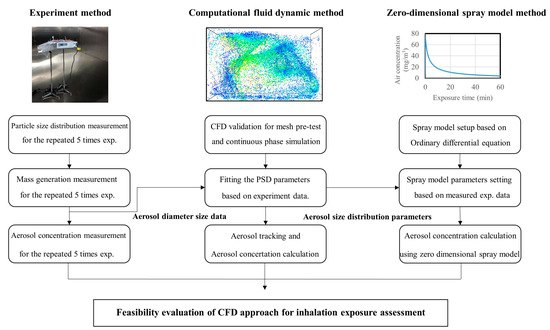
Figure 1.
Research flow chart. The CFD and PSD mean computational fluid dynamics and particle size distribution, respectively.
2. Methods
2.1. Zero-Dimensional Spray Model
The zero-dimensional spray model simulation was performed to assess the applicability of CFD for the inhalation exposure assessment of biocide spray. The zero-dimensional spray model has been developed to predict the biocide concentration results from consumer spray products. The spray model was developed considering the effect of ventilation and the force balance acting on particles by the aerosol diameter size. The spray model [4] is as follows:
where is the ventilation rate, is the total mass of sprayed aerosol/particle (kg), is the aerosol diameter, is the surface area of the room for deposition effect, is the room volume, is the rate of release of mass in aerosol particles, is the rate of non-volatile aerosol from volatile aerosol, is the particle mass distribution function at time t determined from the initial distribution , is terminal velocity, which is decided by . , and are input parameters for the zero-dimensional simulation. The input parameters are obtained based on the measurement results. Equations (1)–(3) represent the total mass of sprayed aerosol/particle during spraying, the total mass of sprayed aerosol/particle after spraying and the total concentration in the room, respectively. The first term of Equation (1) represents the removal mechanism by ventilation. It is assumed that the concentration of non-volatile aerosol is dispersed instantly. The second term of Equation (1) represents the removal mechanism by the force balance effect depending on particle size. As a result, the space concentration is calculated through the mass according to each aerosol diameter. The model, represented by ordinary differential equations, can quickly predict the aerosol concentration in indoor spaces. The input parameters used in the zero-dimensional spray model are classified into aerosol characteristics and spatial characteristics.
In this study, in the case of spatial characteristics, a 30 m3 chamber with a controlled air supply was used in the experiment. Air was supplied from 51 inlets with a diameter of 0.03 m. The total air flow rate is 30 m3. The aerosol input parameters of the zero-dimensional model consist of the particle size distribution (PSD), mass generation rate, exposure factor, etc. The PSD is an important input parameter that affects the results of the zero-dimensional spray simulation and CFD simulation because the particle/aerosol behavior depends on particle diameter size. To set the PSD measurement results equally for CFD and zero-dimensional models, the PSD data were converted to a Rosin–Rammler curve. The RosinRammler curve can describe the PSD by using parameters such as the mean aerosol/particle diameter and spread number. The Rosin–Rambler equation is as follows [25]:
where is the cumulative mass fraction, bigger than a given particle/aerosol diameter , is the mean of particle/aerosol diameter and is the spread number. In other words, the PSD was described by the Rosin–Rammler function. The mean diameter of the particle/aerosol and the spread parameter were determined by curve fitting the experimental results to the Rosin–Rammler function.
The PSD experimental results for the aerosol from biocide spray was obtained by using GRIM OPC equipment, which can be measured in 32 channels from 0.1 μm to 30 μm. In order to take into account the uncertainty, the obtained experimental values were averaged for the results repeated 5 times. Figure 2a represents the mass fraction by the diameter of the particle/aerosol. The mass fraction results in Figure 2a were converted to the cumulative mass fraction curve. Figure 2b represents the experimental and fitted cumulative mass fraction curve. A minimum aerosol diameter size of 0.1 m, size of 15.4 m, maximum aerosol diameter size of 30 m and value of 1.55 were used as the input conditions of the zero-dimensional spray simulation and CFD simulation. The mass generation rate determines the total aerosol concentration that occurs in the spray experiment. The mass generation rate was measured by the weight before and after dispensing. The mass generation rate results were averaged for the results repeated 5 times. In addition, various parameters were also set to simulate the zero-dimensional model, such as the spray time, simulation time and exposure factor. The spray model parameters are shown in Table 1. The measured PSD and mass generation rate were connected equally to the zero-dimensional model and CFD model.
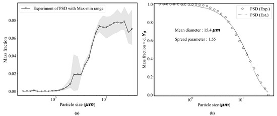
Figure 2.
Results of measurement for mass fraction by aerosol diameter (a) and experimental and fitted cumulative mass fraction curve by aerosol diameter (b). The aerosol size distribution was measured as a repeated method. Mean of PSD for aerosol was converted to a Rosin–Rambler curve to obtain the aerosol information, such as mean of aerosol diameter and spread number.

Table 1.
ConsExpo spray model parameters.
2.2. Measurement of the Sprayed Biocide Concentration
To evaluate the applicability of CFD for the assessment of inhalation exposure from biocide sprays, the concentration of aerosols sprayed in the chamber was measured in various spots in the chamber. The aerosol concentrations in the chamber were measured at six positions to rationally analyze the results of the zero-dimensional spray model and CFD model. The measurement positions and chamber dimensions are shown in Figure 3. The sprayed aerosol concentration was measured five times in a well-controlled chamber to account for the uncertainty. The measurement lasted 60 min after the aerosol was sprayed. The concentration of aerosol was obtained by integration of the mass by particle size distribution measured by using the GRIMM OPC equipment.
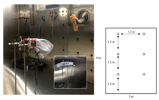
Figure 3.
Experiment setup, measurement positions and chamber dimensions. The experiment was performed in a ventilation chamber of 30 .
2.3. Numerical Simulatiom
Three-dimensional numerical simulations were performed to evaluate the feasibility of the new approach to the inhalation exposure assessment of biocide spray. For estimating the inhalation exposure by biocide spray, a model was used to capture the turbulence flow in an indoor chamber, and the discrete phase model (DPM) was used to track the aerosol dynamic behavior. Additionally, the particle source in cell (PSI-C) algorithm by user define function (UDF) was adopted for calculating the sprayed aerosol concentration. The numerical simulations were conducted by using the commercial CFD solver (ANSYS FLUENT).
2.3.1. Modeling the Flow Field
The sprayed biocide aerosol has a micro-sized diameter. The micro-sized aerosol is dependent on the flow field [26]. In the indoor air flow, a complex three-dimensional turbulent flow is generated. Therefore, it is important to capture the turbulence flow in indoor spaces in order to investigate the biocide aerosol behavior. For numerical simulations of turbulent behavior, the 3D Reynolds average Navier–Stokes (RANS) equation was solved based on the finite volume method. The RANS equation is as follows:
where the Reynolds stress tensor can be defined as:
Here, and are the mean velocity and fluctuating velocity, respectively, and is the pressure of fluid. The Reynolds stress tensor due to turbulence behavior is solved by adopting turbulence models, such as , , Reynold stress model (RSM), etc. Since the flow field is different depending on the turbulence models, an appropriate turbulence model should be used [25,26,27].
It has been proven that the , that assumes the Boussinesq eddy viscosity can capture the flow circulating in an indoor chamber relatively better than the RSM model. The showed slightly better results than the model [14]. The RSM assuming the Reynolds stress tensor with three-dimensional anisotropic property predicted strong circulating flow. Therefore, in this work, we use the model for evaluating the feasibility of the CFD approach for the inhalation exposure assessment in this study. The equation of the model is well described in the following references [27,28].
2.3.2. Modeling the Aerosol Motion
The biocide aerosol motion in an indoor chamber was investigated by an Eulerian–Lagrangian approach, which considers the air flow as a continuous phase, and the aerosols as a dispersed phase. The sprayed biocide aerosol is transported in the continuous phase. The sprayed aerosols were sufficiently diluted so that they did not affect the air flow, and particle-to-particle interactions were not considered in aerosol behavior. In addition, the aerosols were assumed to be non-volatile particles. The micro-sized liquid aerosols of the consumer product spray are volatized into the solid phase rapidly [2]. Therefore, the DPM is suitable for application in the simulations of spray dynamic behavior. To simulate the sprayed biocide aerosol dynamic behavior, the discrete phase model (DPM) was used [25]. The particle-tracking equation is as follows:
where is the particle velocity, is the fluid velocity, is the turbulent velocity fluctuation, is the density of the particle, is the density of fluid, the term FD is the drag force per unit of particle mass and F is an additional acceleration (force/unit particle mass).
Although real turbulence flows apply random movements to particles, the RANS model cannot solve all small turbulence flows due to the averaged effect. The particle trajectory is affected by turbulent velocity fluctuations. The probabilistic tracking method is used to deal with the turbulent velocity fluctuation. The probabilistic tracking method was used to accurately predict the particle behavior with the DPM [25]. In this work, the DPM with a stochastic particle-tracking method was used. The description of the governing equations of the DPM are detailed in the following references [25,28] due to the repeated explanation.
2.3.3. Modeling the Aerosol Concentration
The DPM with a Lagrangian method does not provide functionality for the calculation of aerosol concentration. The particle source in cell (PSI-C) algorithm based on UDF of FLUENT was applied to calculate the aerosol concentration in the specific location. The PSI-C method was developed with the DPM variables. The PSI-C is as follows:
where is the average aerosol concentration in a cell, represents the mass flow rate, the subscript () means the ith tracking particle and the jth cell, respectively, is the aerosol resident time, is the cell volume. The PSI-C code is represented in Figure 4.
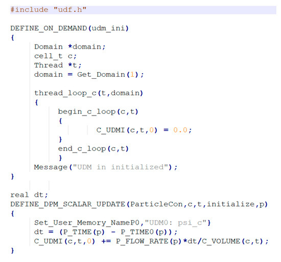
Figure 4.
Particle source in cell (PSI-C) user define function (UDF) code.
2.3.4. Numerical Setting and Domain
Before evaluating the applicability of CFD for the assessment of inhalation exposure from biocide spray, two preliminary tests were conducted to set the suitable simulation condition. The first is the solution convergence test on the aerosol dynamic behavior simulation and the second is the grid test.
In the solution convergence test of the first preliminary test, the residuals of the mass, momentum and turbulence equation did not decrease below 10−3 when transient analysis was used. So, as a solution convergence strategy, in the first step, we used a steady-state solution using the k-epsilon model as an initial guess to provide the solution stability. Then, transient analysis was performed using the with a second-order upward discretization method. It was confirmed that the residuals of the mass, momentum and turbulence equations were reduced to less than 10−5 by the solution convergence strategy. Up to ten iterations were used to converge each time step. The SIMPLE algorithm, PRESTO and second-order upwind scheme were used for the pressure term, pressure–velocity term and turbulence kinetic and dissipation and momentum term, respectively. The criteria of residual values of the turbulence equation and mass/momentum equation for assessing CFD convergence were set as 10−5 and 10−5.
For the grid dependence test of the second preliminary test, the measurement results of a velocity distribution in an indoor chamber were cited by considering time/cost. The grid type is the hexahedron type. The near-wall treatment was achieved by using the scalable wall functions considering the grid refinement with y+ > 11.126. The grid independence test was conducted by comparing the velocity profile CFD results of three types of mesh (coarse, moderate and fine) with the velocity profile measurement results [14] to derive the optimal grid size. The optimized grid size is applied to the simulation conditions of this work for the biocide spray simulation. The total number and mesh size of the coarse type are 3.5 × 10⁵ and 0.05 m, respectively. The total number and mesh size of the moderate type are 2.8 × 10⁶ and 0.015 m, respectively. The total number and mesh size of the fine type are 7.5 × 10⁶ and 0.007 m, respectively. The Figure 5 shows the result of the grid dependence test. As a result of comparing the velocity profile measured at three locations 0.2 m, 0.4 m and 0.6 m from the wall with simulated results by changing the grid size, it can be seen that the chamber flow can be efficiently predicted when a maximum length of the grid of 0.015 m is used. The mesh size has a reasonable computational cost and high accuracy. Therefore, in this study, the maximum length of grid was set to 0.015 m.
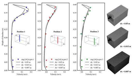
Figure 5.
Mesh independence results. The experiment data were cited in [14]. The max length of the grid is decreased to 0.05, 0.015 and 0.007 m. The measurement positions are 0.2, 0.4 and 0.5 m from the wall.
So, based on preliminary tests results, in this work, the model was used to capture the turbulence flow in an indoor chamber, and the discrete phase model (DPM) was used to track the aerosol dynamic behavior. In addition, the particle source in cell (PSI-C) algorithm by UDF with DPM variables was adopted for calculating the sprayed aerosol concentration. The three modeling methods can be applied to estimate the inhalation exposure from biocide spray.
2.3.5. Numerical Method for Exposure Assessment of Aerosol Concentration by Biocide Spray
We investigated the feasibility of applying CFD for the evaluation of inhalation exposure to solve the spatial problem of zero-dimensional spray models and the time/cost problem of experimental methods. First, we investigated the underestimation possibility of exposure estimation by the zero-dimensional spray model based on CFD and measurement results. Then, the CFD results of the sprayed aerosol concentration in various positions were compared with actual measurement results in order to investigate the CFD applicability for the inhalation exposure assessment of the sprayed biocide aerosol, considering the time/cost problem of experimental methods.
The measurement position, boundary condition and computation mesh domain of the chamber used in this study are shown in Figure 6. The computation mesh was generated as a hexahedron type. The green box was called the near field, and is 1 m3. The other area is called the far field. The zones were used to investigate the possibility of the underestimation of exposure estimation due to the spatial problem of the zero-dimensional spray model. The aerosol was sprayed in the center of the near field for 3 s. The aerosol parameters, such as PSD and mass generation rate, were used in the obtained measurement results in Section 2.3.1. As for the aforementioned solution stability strategy, the continuous phase was first simulated for 2000 iterations in steady state. Then, the transient simulation was followed with a DPM combined with a PSC-I method for 3600 s. The micro-sized liquid aerosols from the consumer product spray are volatized into the solid phase rapidly [2]. Therefore, the DPM is suitable for application in the simulation of spray dynamic behavior. The CFD setup for the model, boundary condition and DPM condition used in this study are summarized in Table 2 and Table 3. The aerosols with large diameters quickly settle on the floor [2]. To consider this effect, we set the trap DPM boundary conditions that terminate particle tracking when the aerosol contacts the floor. In addition, wall boundary conditions were set, except for inlet and outlet, shown in Figure 6.
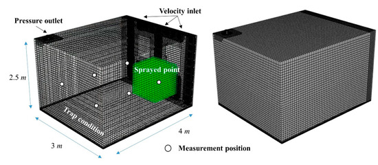
Figure 6.
The measurement position, boundary condition and computation mesh domain of the chamber. The computational domain is divided into near field (green) and far field for validating the zero-dimensional spray model.
Table 2.
CFD parameters for simulation.
Table 3.
Discrete particle method (DPM) parameters for simulation.
3. Results
3.1. Evaluation on the Underestimation Possiblity of Inhalation Exposure by Zero-Dimensional Spray Model Based on CFD and Experiment Results
The possibility of underestimation by the zero-dimensional spray model was confirmed in two steps. The first step was to evaluate the zero-dimensional spray model while verifying the validity of the CFD analysis based on the experimental results. In order to reflect the momentary aerosol spread assumption of the zero-dimensional spray model, the aerosol concentration over the total volume of space (far field) was calculated by using CFD, and the experimental results at six locations were averaged (far field).
In the second step, in order to analyze the possibility of underestimation, the simulated concentration value and the experimental value at a specific location (near field) near the spray were compared with the zero-dimensional spray model results. The aerosol concentration of CFD was calculated over time by using the model, PSI-C method, DPM model and the pre-tested simulation conditions. The CFD simulation time is the same as the experiment and zero-dimensional spray model simulation time. The results of three methods were compared for 3600 s of physics/simulation. The aerosol from the spray was injected for 3 s in the three methods. The aerosol concentration of the zero-dimensional spray model was calculated by solving the ordinary differential equation for spray behavior.
Figure 7a shows the comparison results for the three methods in the far field. As shown in Figure 7a, the spray model results, the experimental results in the far field and CFD in the far field show relatively good results compared to each other. After spraying, the aerosol concentration decreases rapidly within 5 min because the large-diameter particles quickly fall to the bottom. This phenomenon can be confirmed through the aerosol dynamic behavior result within 5 min by the CFD method in Figure 8a. After 5 min, the micro-diameter aerosol throughout the space is diluted throughout the entire space and removed through the upper outlet by ventilation. When the aerosol is sufficiently diluted, it can be seen that aerosols with small diameters are circulated throughout the space depending on the flow velocity field, shown in Figure 8b.
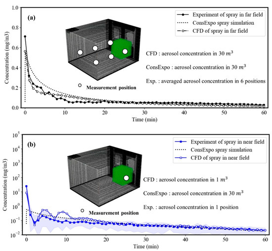
Figure 7.
The comparison results of experimental results, zero-dimensional spray simulation (ConsExpo simulation) and CFD simulation in near field and far field. (a) Far field comparison results, (b) near field—far field comparison results.
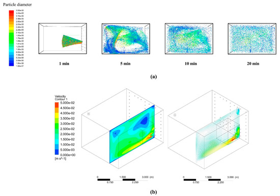
Figure 8.
The dynamic behavior of sprayed biocide aerosol over simulation time (a). Visualization of velocity contour and vector in chamber (b). The dynamic behavior of sub-micro aerosol is dependent on turbulence flow.
Figure 7b represents the result of comparing the CFD result of aerosol concentration and the aerosol concentration measurement result in the near field with the result of the zero-dimensional spray model. Figure 7b shows that the CFD aerosol concentration results at a specific location and the experimental aerosol concentration values differ from that of the zero-dimensional spray model. This is a phenomenon caused by aerosol propagation, as shown in Figure 8a. The CFD results in the near field show similarity to the mean-max experimental results in near field over time. That is, the zero-dimensional spray model that ignores spatial characteristics can predict the results contrary to the actual exposure evaluation depending on the location, and the CFD method can explain the aerosol propagation caused by the actual turbulence well.
In addition, Table 4 shows the exposure concentration of the time-weight average by the spray model, CFD modeling and experimental method. The spray model is underestimated by approximately five times when compared with the CFD results in the near field. We quantitatively show that the CFD results of exposure in the near field are similar to the measurement results in near field. Therefore, it can be seen that CFD and experimental methodologies, taking into account spatial characteristics, are needed for proper inhalation exposure assessment.
Table 4.
Time-weight averaged aerosol concentration for experimental results in near field and far field, CFD results in near field and far field and ConsExpo simulation.
3.2. Evaluation on the Feasibility of CFD for Inhalation Exposure Assessment Based on Experimental Results
The measurement results of the concentration of aerosols at five locations and the CFD results at the same five locations were compared to solve the experimental problem of time/cost and to evaluate the possibility of inhalation exposure at various locations by using CFD. The five measurements are at positions other than the near field. The measurement data where the aerosol concentration rises the most at each measurement location were compared with the CFD results of the same time and location, as shown Figure 9.
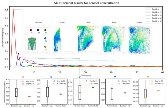
Figure 9.
Comparison of measurement result with CFD results in the five measurement positions. The error bar is used due to repeated experiments. The circle is the average of the measurement results, which is the peak concentration. The CFD results according to the measurement position are similar to the measurement results.
The aerosol concentrations by measurement position due to the aerosol propagation were calculated. The experiment was performed independently five times. The experimental result includes an error bar representing the minimum, mean and maximum with standard deviation. The CFD value at each measurement location is within the experimental error range. This means the CFD conditions such as mesh size, numerical schemes and modeling methods are set correctly. This showed that the concentration of aerosol exposure at various locations can be reasonably evaluated through CFD and that the CFD approach can be successfully applied to exposure estimation.
4. Conclusions
In this paper, we investigated the applicability of CFD for inhalation exposure assessment from biocide spray in order to solve the spatial problem of the zero-dimensional space model and the time/cost-consuming problem of measurement methods. The CFD results of the sprayed aerosol concentration in various positions were compared with measurement results and the zero-dimensional spray model results. The results of the three methods were compared for 3600 s of physics/simulation. The conclusions can be drawn as follows:
(1) The zero-dimensional spray model results, the experimental results in the far field and CFD in the far field show relatively good results when compared to each other. However, the spray model shows an underestimation of approximately five times when compared with the CFD results in the near field and experimental results in the near field. In this study, it was shown that exposure evaluation should be performed using CFD or experimental methods rather than the conventional zero-dimensional model.
(2) When the concentration measurement is performed at various locations using experimental methodology, the cost generated and time required are enormous. The results of measuring the concentration of aerosols at five locations and the CFD results at the same location were compared to show the possibility of evaluating inhalation exposure at various locations using CFD. The experimental result includes an error bar representing the minimum, average and maximum. It can be seen that the CFD value at each measurement location is within the experimental error range. In this study, it was shown that the experimental cost and time problem for inhalation exposure can be reasonably solved using CFD.
In other words, in the field of exposure science, a guideline for exposure evaluation using CFD was found that complements the shortcomings of the conventional methodology, the zero-dimensional spray model and measurement method.
However, CFD generates a relatively high computational cost for the simulation of exposure estimation. It is difficult to estimate the exposure according to the user’s needs. To address these computational cost problems, machine learning modeling methods based on simulation data are used in various industries [29,30,31]. Therefore, in future research, we will develop a machine learning model with spatial information as an input variable and spatial concentration as an output variable to predict concentration according to various spatial structures and characteristics.
Author Contributions
D.P. analyzed the numerical data and organized the draft paper; J.-H.L. performed the experiment. All authors have read and agreed to the published version of the manuscript.
Funding
This research was supported by the Korea Environment Industry & Technology Institute (KEITI) through the Environmental Health Action Program, funded by the Korean Ministry of Environment (MOE) (No. 2012001370007, NTIS 1485012429.
Institutional Review Board Statement
Not applicable.
Informed Consent Statement
Informed consent was obtained from all subjects involved in the study.
Data Availability Statement
The data presented in this study are available on request from the corresponding author.
Conflicts of Interest
The authors declare no potential conflict of interest with respect to the research, authorship and publication of this article.
References
- RIVM. ConsExpo Nano Tool. Available online: www.consexponano.nl.www.consexpoweb.nl (accessed on 30 October 2007).
- RIVM. Consexpo Web. Available online: www.consexpoweb.nl (accessed on 30 October 2016).
- US EPA. Consumer Exposure Model (CEM) User Guide. Available online: www.epa.gov/sites/production/files/2019-06/documents/cem_2.1_user_guide.pdf (accessed on 11 December 2019).
- Delmaar, J.E.; Bremmer, H.J. Modeling and Experimental Validation of the Inhalation Exposure of Consumers to Aerosols from Spray Cans and Trigger Sprays; RIVM: Utrecht, The Netherlands, 2009. [Google Scholar]
- Young, B.M.; Tulve, N.S.; Egeghy, P.P.; Driver, J.H.; Zartarian, V.G.; Johnston, J.E.; Barnekow, D.E. Comparison of four probabilistic models (CARES®, CalendexTM, Zero-dimensional, and SHEDS) to estimate aggregate residential exposures to pesticides. J. Expo. Sci. Environ. Epidemiol. 2012, 22, 522–532. [Google Scholar] [CrossRef] [PubMed]
- Arnold, S.F.; Ramachandran, G. Influence of parameter values and variances and algorithm architecture in ConsExpo model on modeled exposures. J Occup. Environ. Hyg. 2014, 11, 54–66. [Google Scholar] [CrossRef] [PubMed]
- Delmaar, C.; Meesters, J. Modeling consumer exposure to spray products: An evaluation of the ConsexpoWeb and Consexponano models with experimental data. J. Expo. Sci. Environ. Epidemiol. 2020, 30, 878–887. [Google Scholar] [CrossRef] [PubMed]
- Park, J.; Yoon, C.; Lee, K. Comparison of modeled estimates of inhalation exposure to aerosols during use of consumer spray products. Int. J. Hyg. Environ. Health 2018, 221, 941–950. [Google Scholar] [CrossRef]
- Kwon, K.S.; Lee, I.B.; Han, H.T.; Shin, C.Y.; Hwang, H.S.; Hong, S.W.; Bitog, J.P.; Seo, I.H.; Han, C.P. Analysing ventilation efficiency in a test chamber using age-of-air concept and CFD technology. Biosyst. Eng. 2011, 110, 421–433. [Google Scholar] [CrossRef]
- Cherrie, J.W.; MacCalman, L.; Fransman, W.; Tielemans, E.; Tischer, M.; Van Tongeren, M. Revisiting the effect of room size and general ventilation on the relationship between near- and far-field air concentrations. Ann. Occup. Hyg. 2011, 55, 1006–1015. [Google Scholar] [CrossRef]
- Park, D.; Cha, J.; Kim, M.; Go, J.S. Multi-objective optimization and comparison of surrogate models for separation performances of cyclone separator based on CFD, RSM, GMDH-neural network, back propagation-ANN and genetic algorithm. Eng. Appl. Comput. Fluid Mech. 2020, 14, 180–201. [Google Scholar] [CrossRef]
- Cha, J.; Kim, M.; Park, D.; Go, J.S. Experimental determination of the viscoelastic parameters of K-BKZ model and the influence of temperature field on the thickness distribution of ABS thermoforming. Int. J. Adv. Manuf. Technol. 2019, 103, 985–995. [Google Scholar] [CrossRef]
- Liu, Z.; Li, A.; Xu, X.; Gao, R. Computational fluid dynamics simulation of airflow patterns and particle deposition characteristics in children upper respiratory tracts. Eng. Appl. Comput. Fluid Mech. 2012, 6, 556–571. [Google Scholar] [CrossRef]
- Chen, F.; Yu, S.C.M.; Lai, A.C.K. Modeling particle distribution and deposition in indoor environments with a new drift-flux model. Atmos. Environ. 2006, 40, 357–367. [Google Scholar] [CrossRef]
- He, X.; Xu, H.; Li, W.; Sheng, D. An improved VOF-DEM model for soil-water interaction with particle size scaling. Comput. Geotech. 2020, 128, 103818. [Google Scholar] [CrossRef]
- Xu, L.; Zhou, X.; Li, J.; Hu, Y.; Qi, H.; Wen, W.; Du, K.; Ma, Y.; Yu, Y. Numerical simulations of molten breakup behaviors of a de laval-type nozzle, and the effects of atomization parameters on particle size distribution. Processes 2020, 8, 1027. [Google Scholar] [CrossRef]
- Silva, M.C.F.; Campos, J.B.L.M.; Miranda, J.M.; Araújo, J.D.P. Numerical study of single taylor bubble movement through a microchannel using different CFD packages. Processes 2020, 8, 1418. [Google Scholar] [CrossRef]
- McCraney, J.; Weislogel, M.; Steen, P. OpenFOAM Simulations of Late Stage Container Draining in Microgravity. Fluids 2020, 5, 207. [Google Scholar] [CrossRef]
- Tembely, M.; Alameri, W.S.; Alsumaiti, A.M.; Jouini, M.S. Pore-scale modeling of the effect of wettability on two-phase flow properties for newtonian and non-newtonian fluids. Polymers 2020, 12, 2832. [Google Scholar] [CrossRef]
- Stachnik, M.; Jakubowski, M. Multiphase model of flow and separation phases in a whirlpool: Advanced simulation and phenomena visualization approach. J. Food Eng. 2020, 274, 109846. [Google Scholar] [CrossRef]
- Chang, P.; Xu, G.; Huang, J. Numerical study on DPM dispersion and distribution in an underground development face based on dynamic mesh. Int. J. Min. Sci. Technol. 2020, 30, 471–475. [Google Scholar] [CrossRef]
- Stone, L.; Hastie, D.; Zigan, S. Using a coupled CFD – DPM approach to predict particle settling in a horizontal air stream. Adv. Powder Technol. 2019, 30, 869–878. [Google Scholar] [CrossRef]
- Wang, P.; Zhu, X.; Li, Y. Analysis of Flow and Wear Characteristics of Solid–Liquid Two-Phase Flow in Rotating Flow Channel. Processes 2020, 8, 1512. [Google Scholar] [CrossRef]
- Zhou, Y.; Deng, Y.; Wu, P.; Cao, S.J. The effects of ventilation and floor heating systems on the dispersion and deposition of fine particles in an enclosed environment. Build. Environ. 2017, 125, 192–205. [Google Scholar] [CrossRef]
- ANSYS Inc. ANSYS FLUENT Theory Guide; ANSYS Inc.: Canonsburg, PA, USA, 2018. [Google Scholar]
- Adedoyin, A.A.; Walters, D.K.; Bhushan, S. Investigation of turbulence model and numerical scheme combinations for practical finite-volume large eddy simulations. Eng. Appl. Comput. Fluid Mech. 2015, 9, 324–342. [Google Scholar] [CrossRef]
- Rahimzadeh, H.; Maghsoodi, R.; Sarkardeh, H.; Tavakkol, S. Simulating flow over circular spillways by using different turbulence models. Eng. Appl. Comput. Fluid Mech. 2012, 6, 100–109. [Google Scholar] [CrossRef]
- Tang, Y.; Guo, B.; Ranjan, D. Numerical simulation of aerosol deposition from turbulent flows using three-dimensional RANS and les turbulence models. Eng. Appl. Comput. Fluid Mech. 2015, 9, 174–186. [Google Scholar] [CrossRef]
- Park, D.; Go, J.S. Design of cyclone separator critical diameter model based on machine learning and cfd. Processes 2020, 8, 1521. [Google Scholar] [CrossRef]
- Yang, C.; Kim, Y.; Ryu, S.; Gu, G.X. Prediction of composite microstructure stress-strain curves using convolutional neural networks. Mater. Des. 2020, 189, 108509. [Google Scholar] [CrossRef]
- Kim, Y.; Yang, C.; Kim, Y.; Gu, G.X.; Ryu, S. Designing an Adhesive Pillar Shape with Deep Learning-Based Optimization. ACS Appl. Mater. Interfaces 2020, 12, 24458–24465. [Google Scholar] [CrossRef]
Publisher’s Note: MDPI stays neutral with regard to jurisdictional claims in published maps and institutional affiliations. |
© 2021 by the authors. Licensee MDPI, Basel, Switzerland. This article is an open access article distributed under the terms and conditions of the Creative Commons Attribution (CC BY) license (http://creativecommons.org/licenses/by/4.0/).