Chinese Character Image Completion Using a Generative Latent Variable Model

Abstract
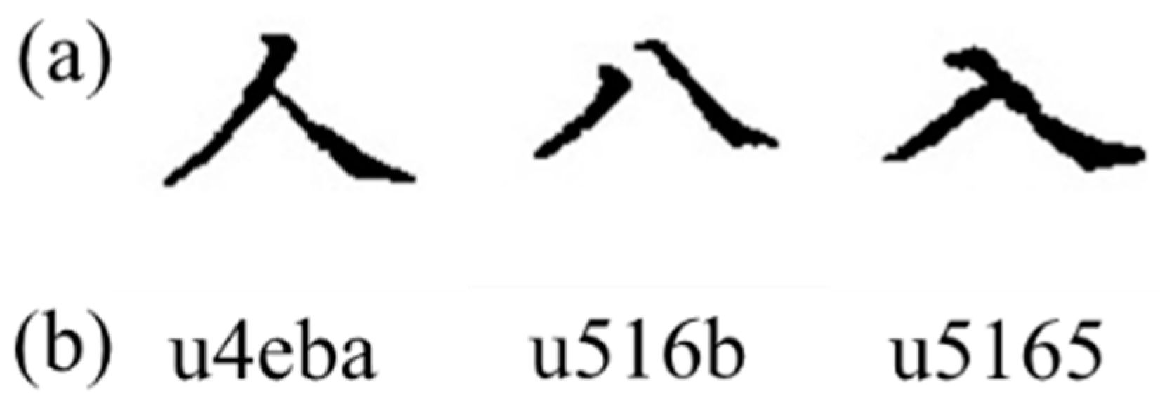
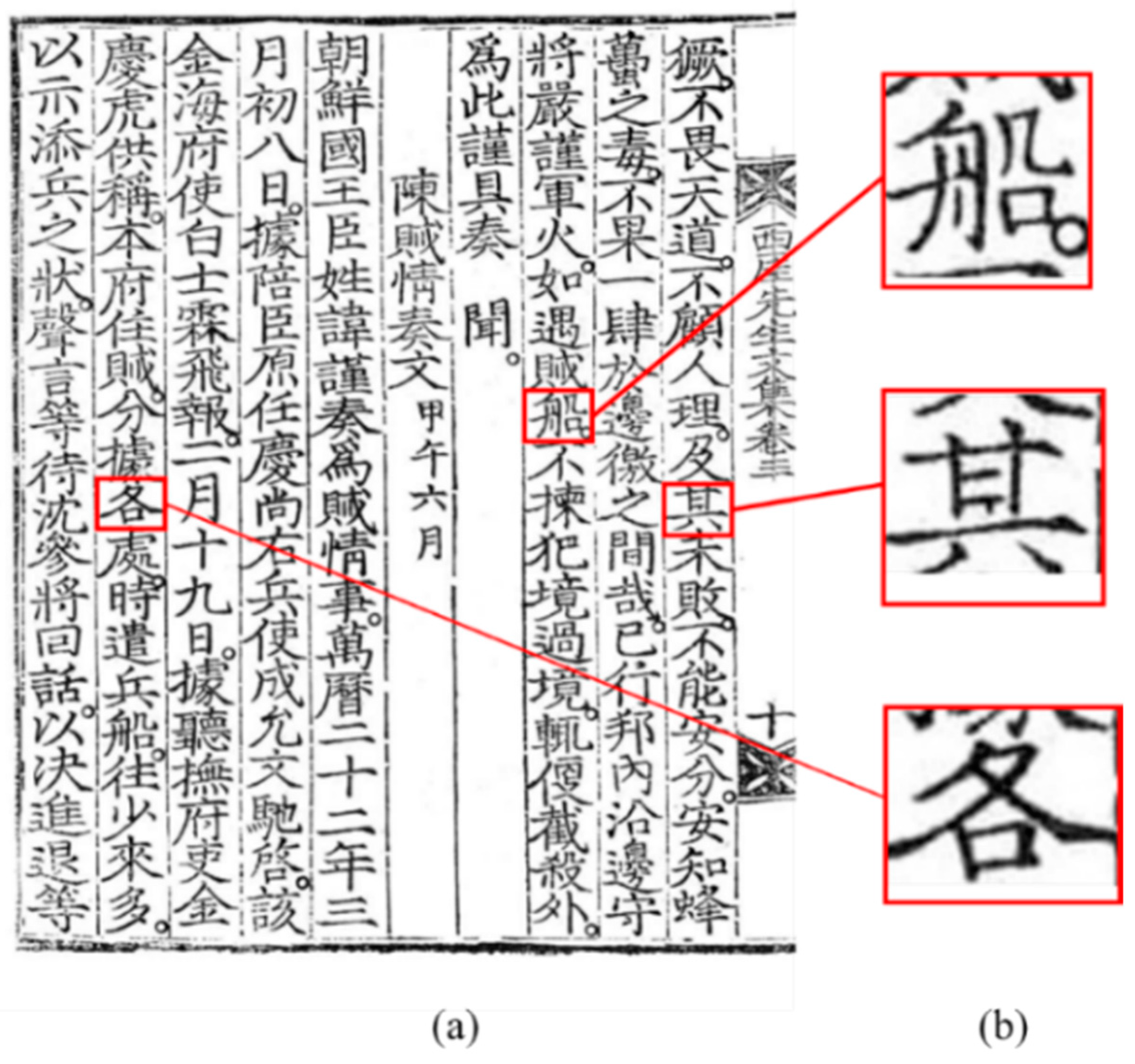
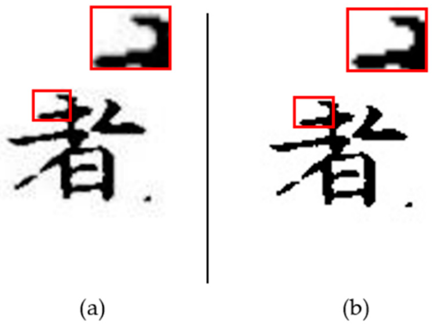
1. Introduction
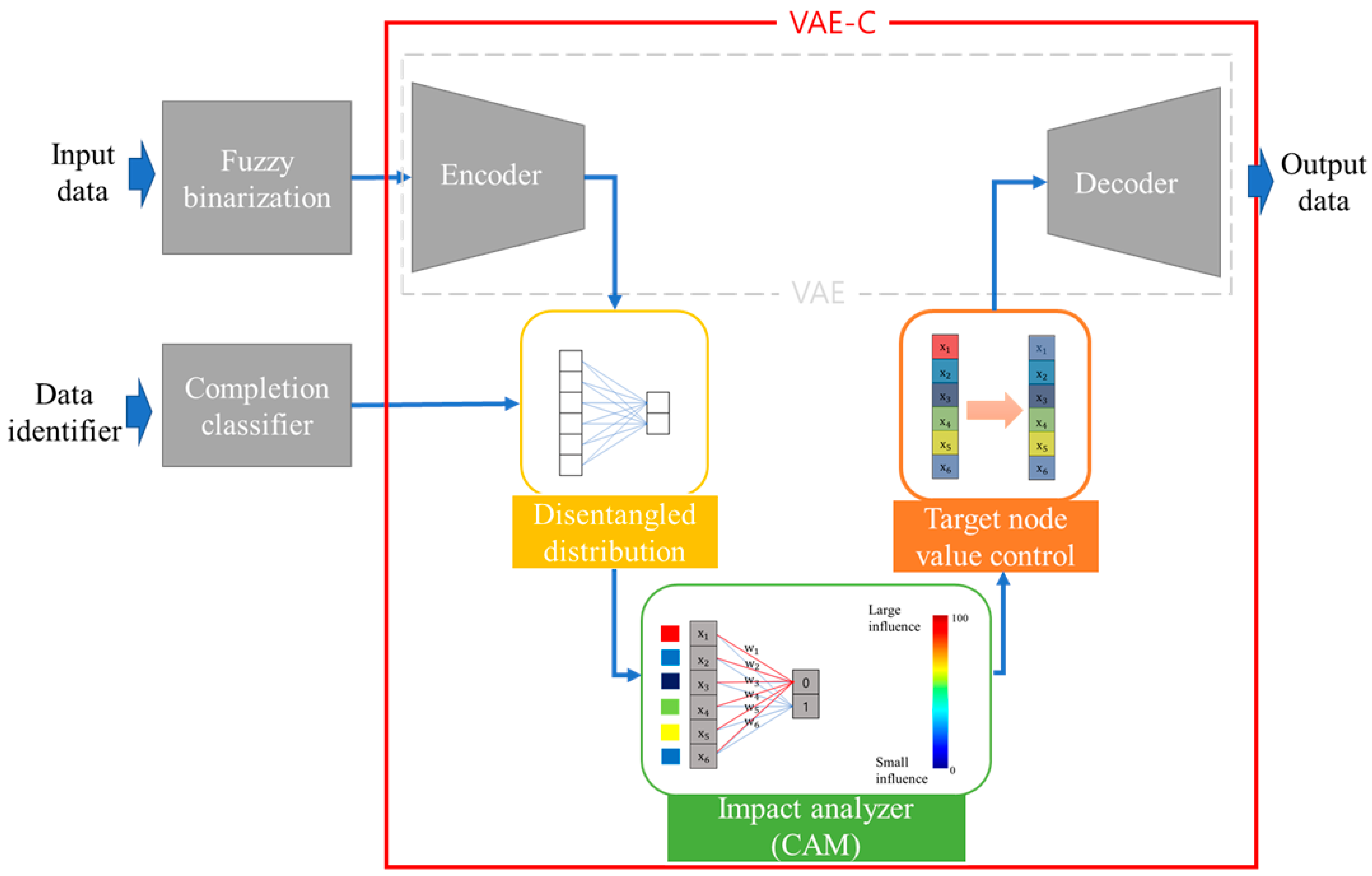
2. Materials and Methods
2.1. Materials
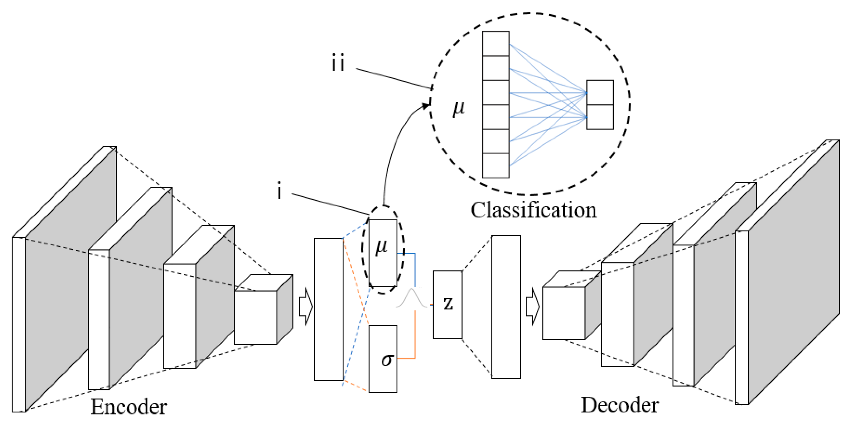
2.1.1. Variational Autoencoder
2.1.2. Class Activation Map
2.2. Methodology
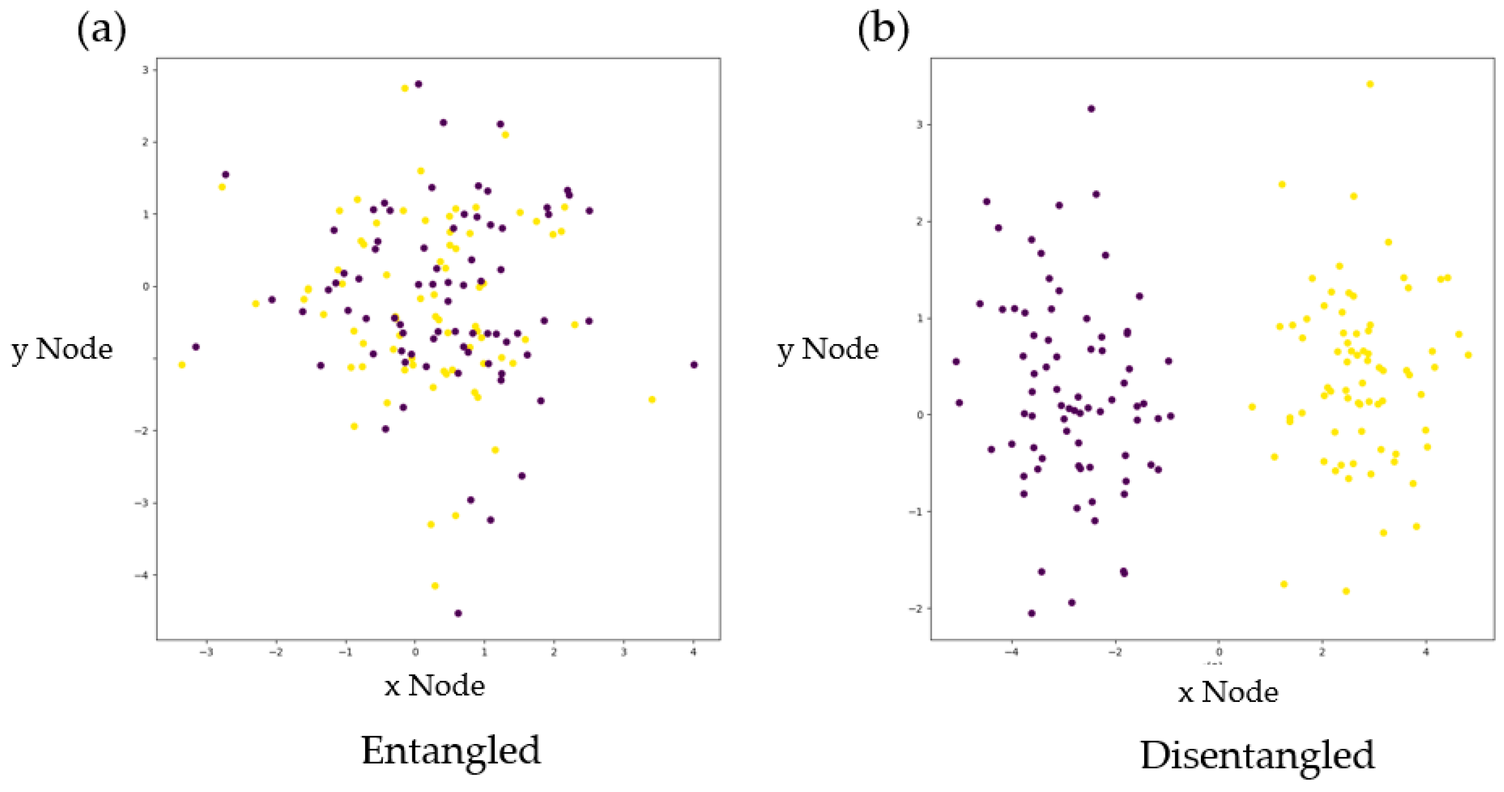
2.2.1. Disentanglement
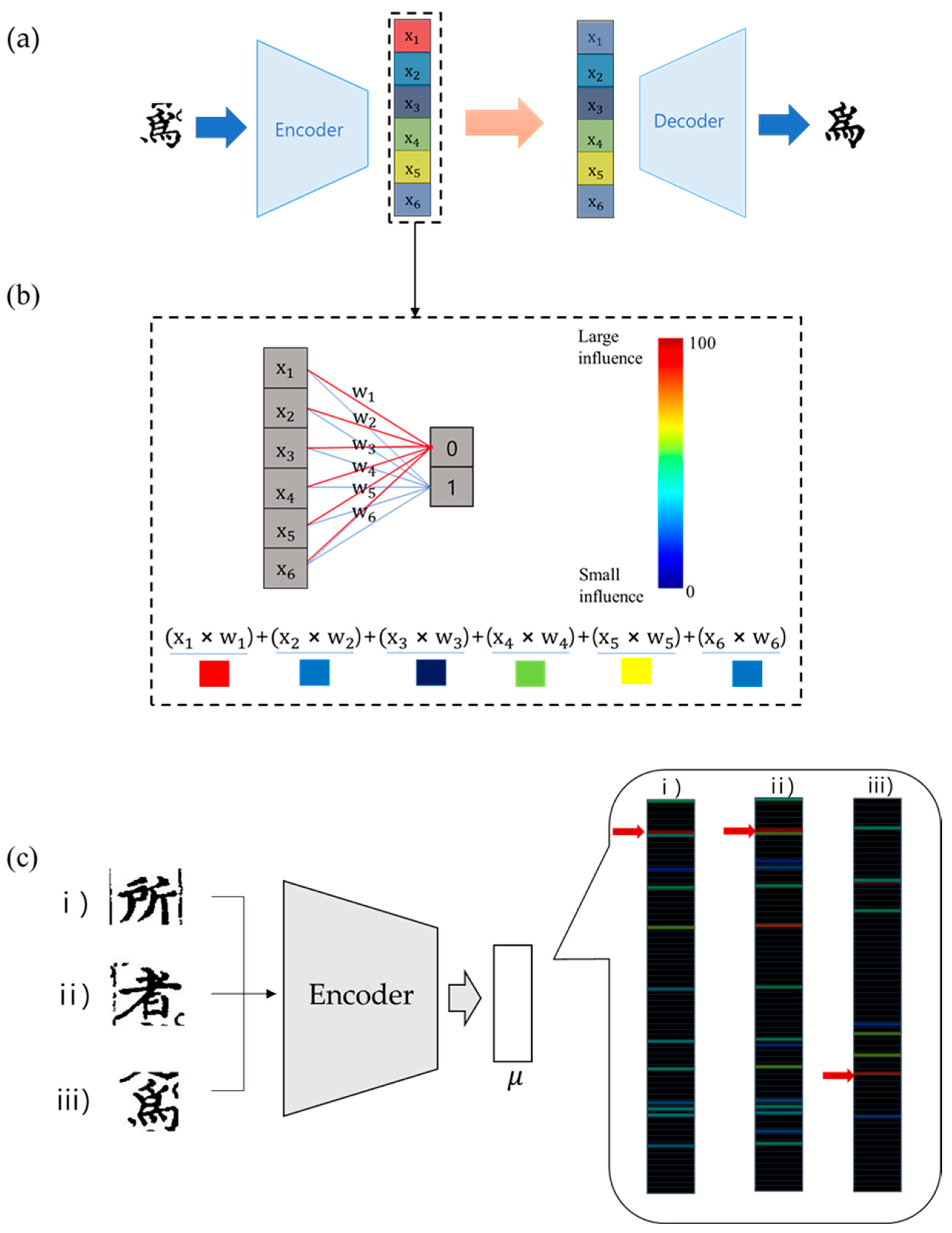
2.2.2. Tracking Nodes Using Class Activation Map
2.3. Model Construction
2.4. Chinese Character Images Dataset
3. Results
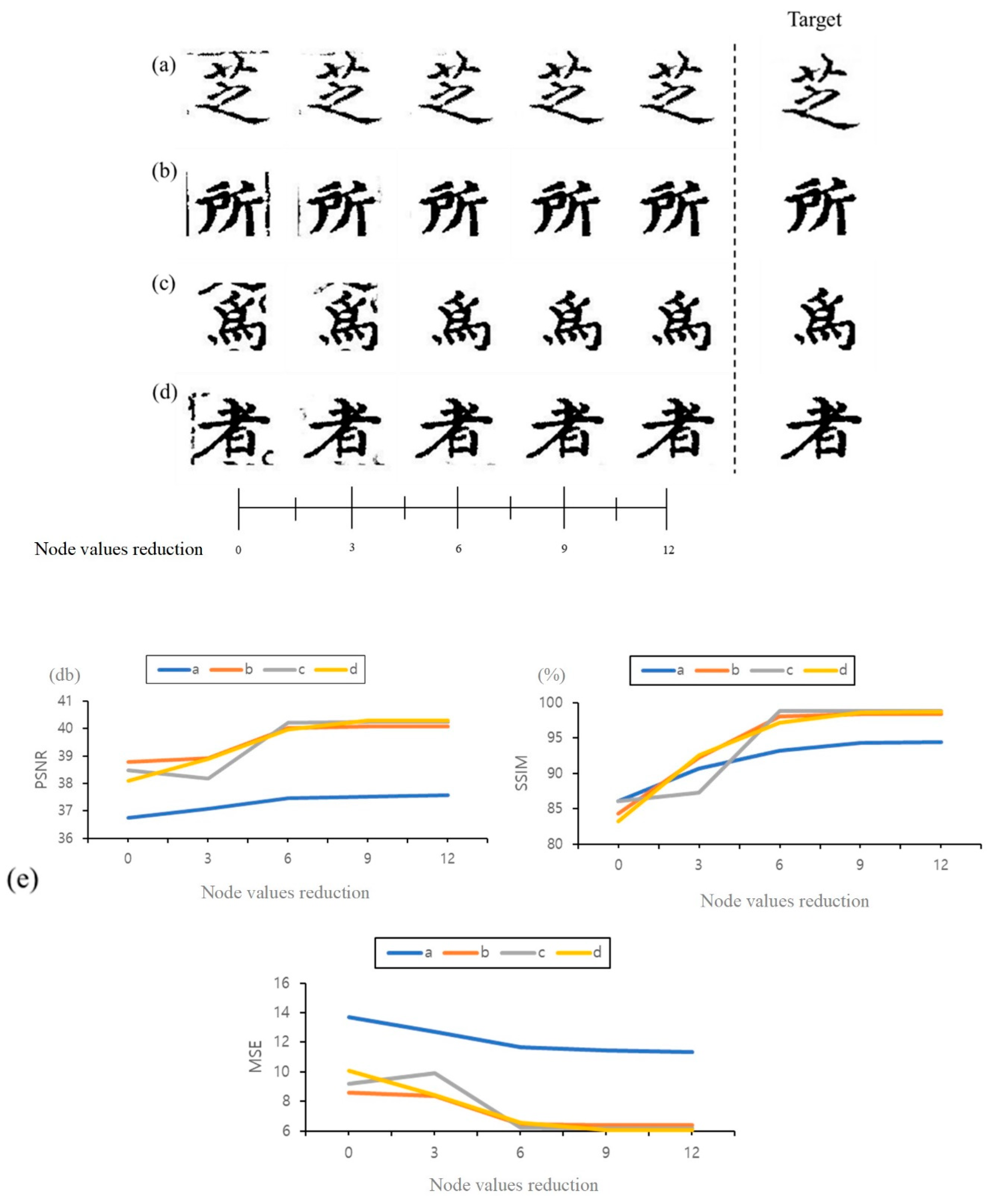
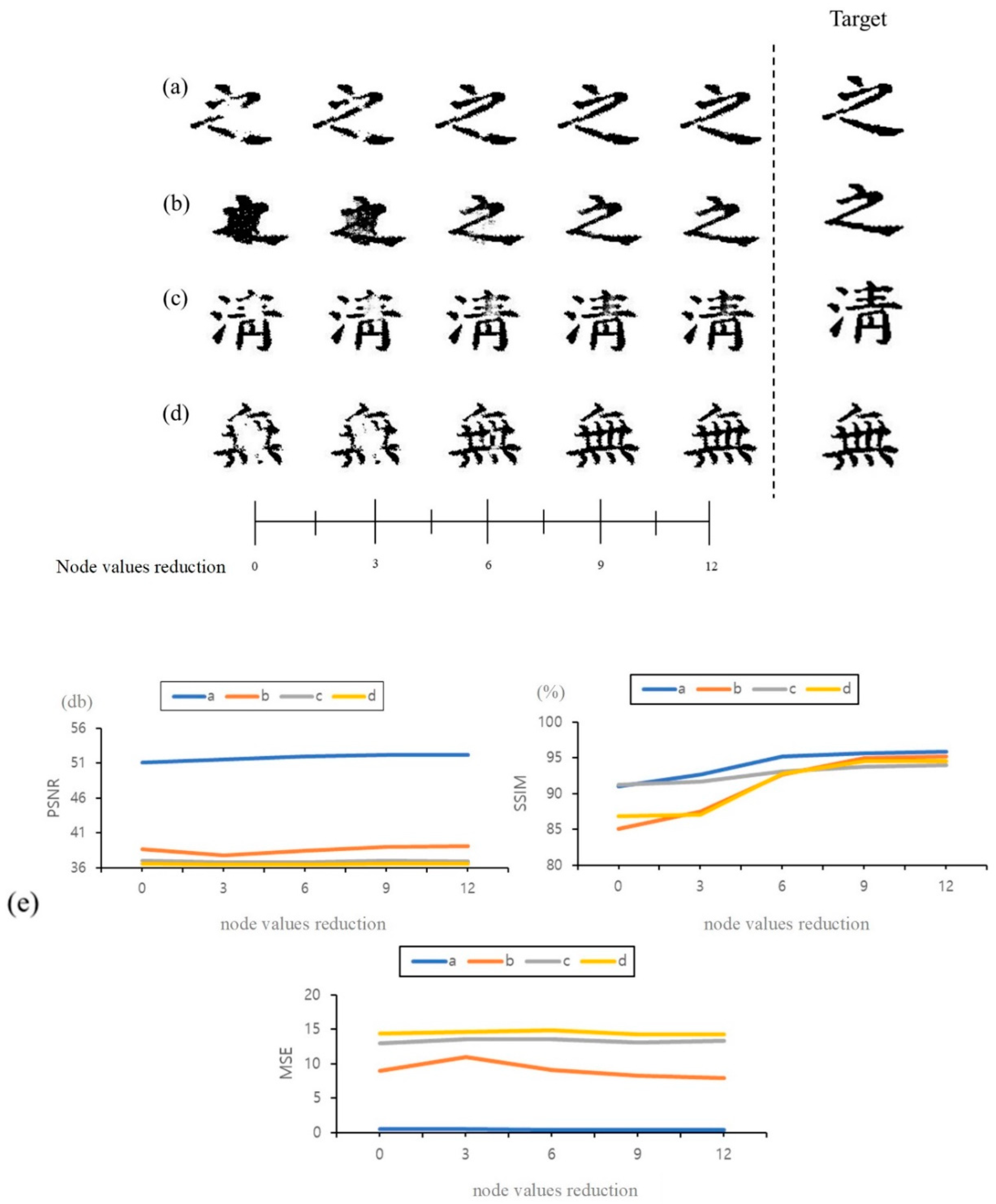
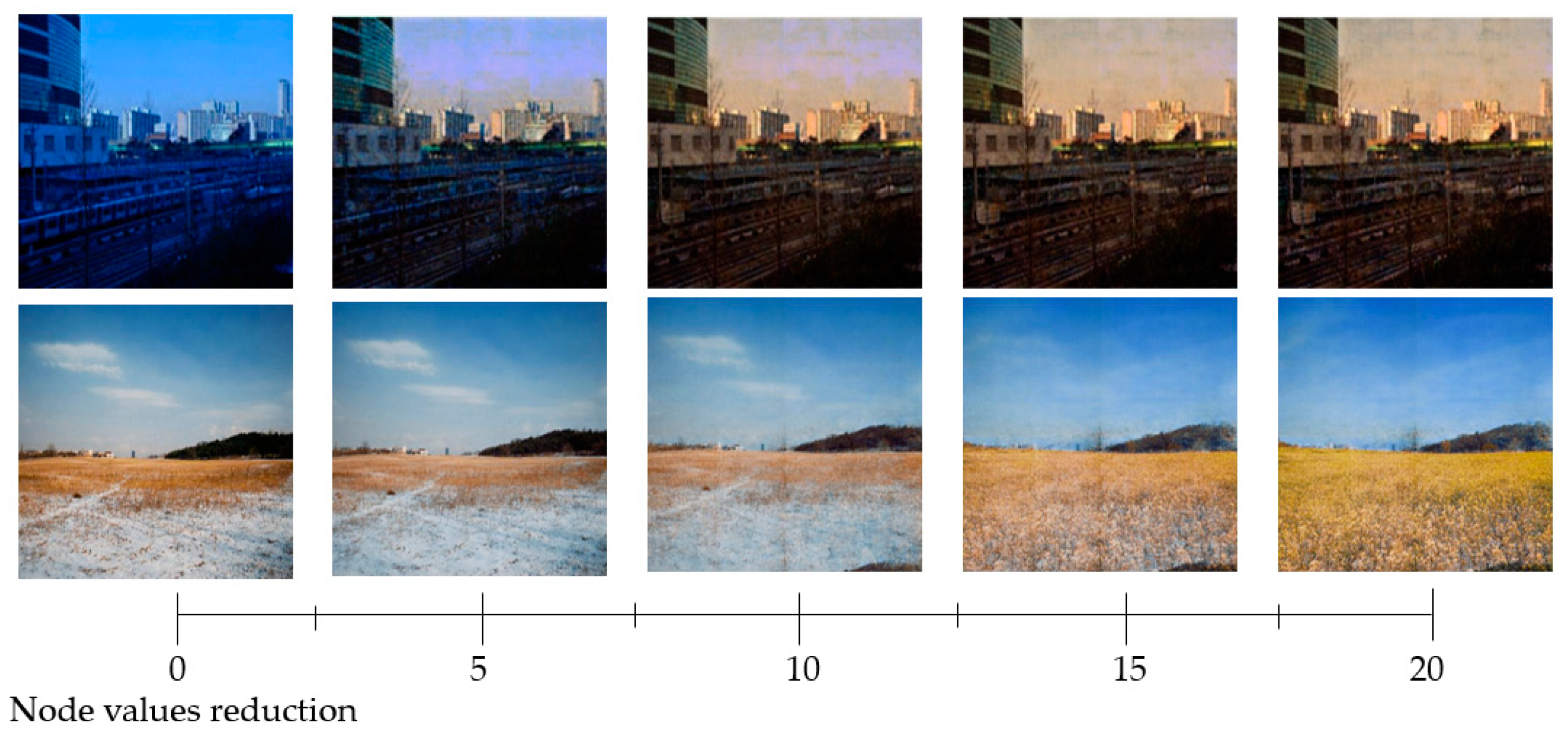
3.1. Variation of Output Value as Node Value Changes
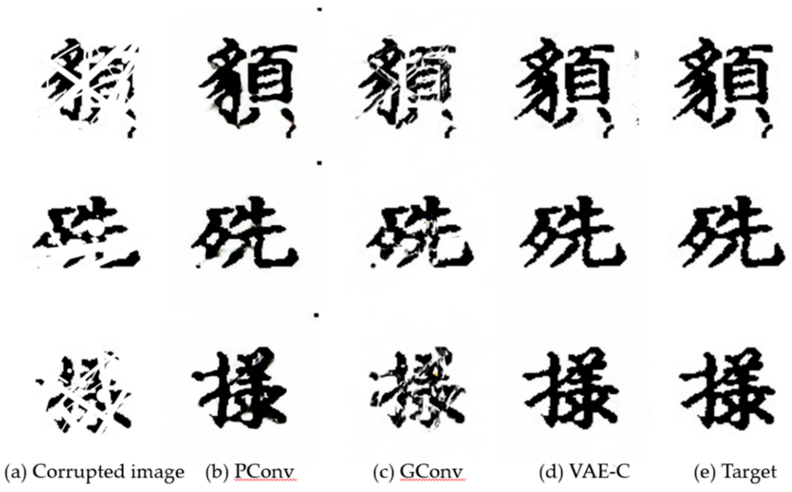
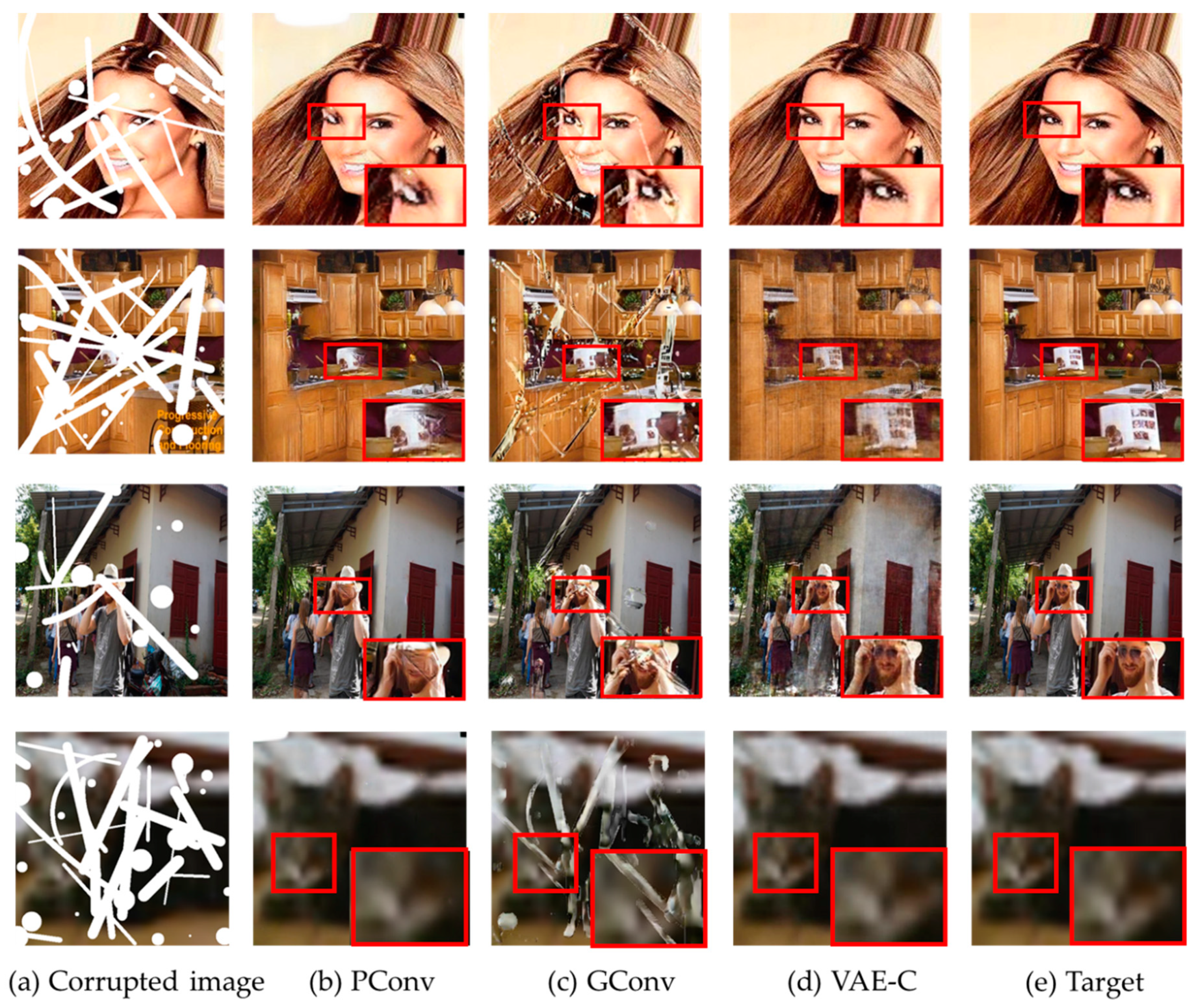
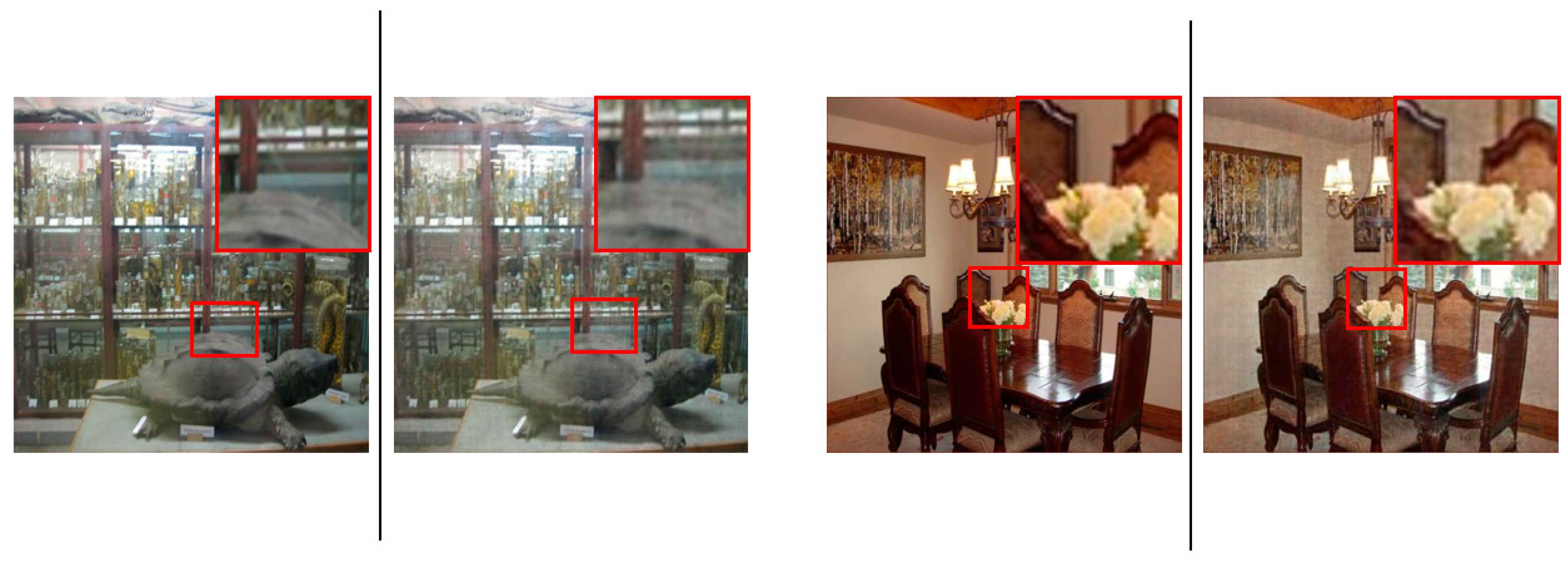
3.2. Image Restoration Performance Comparison
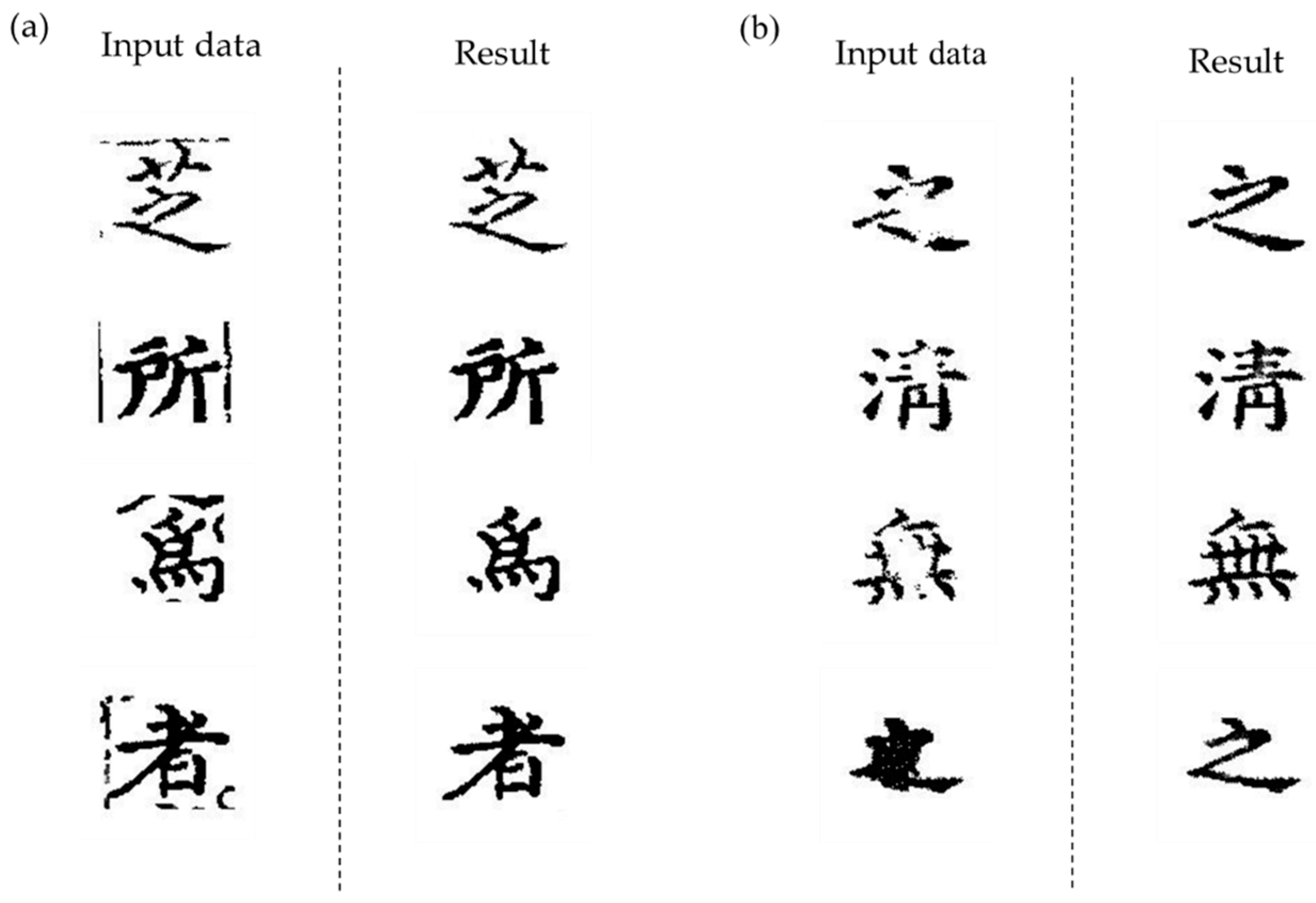
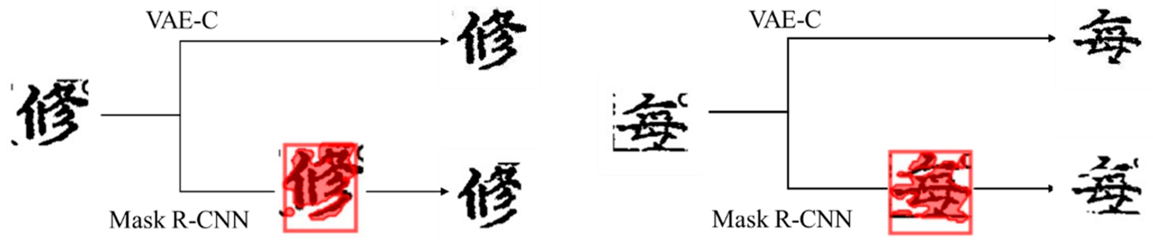
3.3. Object Removal Performance Comparison
4. Discussion
5. Conclusions
Author Contributions
Funding
Institutional Review Board Statement
Informed Consent Statement
Data Availability Statement
Acknowledgments
Conflicts of Interest
References
- Iizuka, S.; Simo-Serra, E.; Ishikawa, H. Globally and locally consistent image completion. ACM Trans. Graph. 2017, 36, 1–14. [Google Scholar] [CrossRef]
- Yu, J.; Lin, Z.; Yang, J.; Shen, X.; Lu, X.; Huang, T. Free-Form Image Inpainting with Gated Convolution. In Proceedings of the 2019 IEEE/CVF International Conference on Computer Vision (ICCV), Seoul, Korea, 1 March 2019; pp. 4470–4479. [Google Scholar]
- Liu, G.; Reda, F.A.; Shih, K.J.; Wang, T.-C.; Tao, A.; Catanzaro, B. Image Inpainting for Irregular Holes Using Partial Convolutions. In Proceedings of the Medical Image Computing and Computer-Assisted Intervention—MICCAI’99, Granada, Spain, 16–20 September 2018; pp. 89–105. [Google Scholar]
- Yu, J.; Lin, Z.; Yang, J.; Shen, X.; Lu, X.; Huang, T.S. Generative Image Inpainting with Contextual Attention. In Proceedings of the 2018 IEEE/CVF Conference on Computer Vision and Pattern Recognition, Salt Lake City, UT, USA, 1–22 June 2018; pp. 5505–5514. [Google Scholar]
- Han, S.; Ahmed, M.U.; Rhee, P.K. Monocular SLAM and Obstacle Removal for Indoor Navigation. In Proceedings of the 2018 International Conference on Machine Learning and Data Engineering (iCMLDE), Sydney, Australia, 3–7 December 2018; pp. 67–76. [Google Scholar]
- Rakshith, S.; Mario, F.; Bernt, S. Adversarial scene editing: Automatic object removal from weak supervision. arXiv 2018, arXiv:1806.01911. [Google Scholar]
- Girshick, R.; Donahue, J.; Darrell, T.; Malik, J. Rich Feature Hierarchies for Accurate Object Detection and Semantic Segmentation. In Proceedings of the 2014 IEEE Conference on Computer Vision and Pattern Recognition, Columbus, OH, USA, 23–28 June 2014; pp. 580–587. [Google Scholar]
- Girshick, R. Fast R-CNN. In Proceedings of the IEEE International Conference on Computer Vision, Santiago, Chile, 7–13 December 2015; pp. 1440–1448. [Google Scholar]
- Ren, S.; He, K.; Girshick, R.; Sun, J. Faster R-CNN: Towards real-time object detection with region proposal networks. IEEE Trans. Pattern Anal. Mach. Intell. 2016, 39, 1137–1149. [Google Scholar] [CrossRef] [PubMed]
- He, K.; Gkioxari, G.; Dollar, P.; Girshick, R. Mask r-cnn. arXiv 2017, arXiv:1703.06870. [Google Scholar]
- Redmon, J.; Divvala, S.; Girshick, R.; Farhadi, A. You only look once: Unified, real-time object detection. arXiv 2015, arXiv:1506.02640. [Google Scholar]
- Zhao, Q.; Sheng, T.; Wang, Y.; Tang, Z.; Chen, Y.; Cai, L.; Ling, H. M2Det: A Single-Shot Object Detector Based on Multi-Level Feature Pyramid Network. Proc. Conf. AAAI Artif. Intell. 2019, 33, 9259–9266. [Google Scholar] [CrossRef]
- Kim, K.-B. ART2 Based Fuzzy Binarization Method with Low Information Loss. J. Korea Inst. Inf. Commun. Eng. 2014, 18, 1269–1274. [Google Scholar] [CrossRef][Green Version]
- Lee, H.C.; Kim, K.B.; Park, H.J.; Cha, E.Y. An a-cut Automatic Set based on Fuzzy Binarization Using Fuzzy Logic. J. Korea Inst. Inf. Commun. Eng. 2015, 19, 2924–2932. [Google Scholar] [CrossRef][Green Version]
- Kingma, D.P.; Welling, M. Auto-encoding variational Bayes. arXiv 2013, arXiv:1312.6114. [Google Scholar]
- Mirza, M.; Osindero, S. Conditional generative adversarial nets. arXiv 2014, arXiv:1411.1784. [Google Scholar]
- Zhang, Z.; Song, Y.; Qi, H. Age progression/regression by conditional adversarial autoencoder. In Proceedings of the IEEE Conference on Computer Vision and Pattern Recognition, Honolulu, HI, USA, 21–26 July 2017; pp. 5810–5818. [Google Scholar]
- Sohn, K.; Lee, H.; Yan, X. Learning structured output representation using deep conditional generative models. Adv. Neural Inf. Process. Syst. 2015, 28, 3483–3491. [Google Scholar]
- Bishop, C.M. Mixture Density Networks; Technical Report; NCRG/94/004; Aston University: Birmingham, UK, 1994. [Google Scholar]
- Hershey, J.R.; Olsen, P.A. Approximating the Kullback Leibler Divergence between Gaussian Mixture Models. In Proceedings of the 2007 IEEE International Conference on Acoustics, Speech and Signal Processing-ICASSP ’07, Honolulu, HI, USA, 15–20 April 2007; Volume 4, p. IV-317. [Google Scholar]
- Zhou, B.; Khosla, A.; Lapedriza, A.; Oliva, A.; Torralba, A. Learning deep features for discriminative localization. In Proceedings of the IEEE Conference on Computer Vision and Pattern Recognition (CVPR), Las Vegas, NV, USA, 27–30 June 2016; pp. 2921–2929. [Google Scholar]
- Selvaraju, R.R.; Cogswell, M.; Das, A.; Vedantam, R.; Parikh, D.; Batra, D. Gradcam: Visual explanations from deep networks via gradient-based localization. In Proceedings of the IEEE Conference on Computer Vision and Pattern Recognition, Venice, Italy, 22–29 October 2017; pp. 618–626. [Google Scholar]
- Zeiler, M.D.; Taylor, G.W.; Fergus, R. Adaptive deconvolutional networks for mid and high level feature learning. In Proceedings of the 2011 International Conference on Computer Vision, Barcelona, Spain, 6–13 November 2011; pp. 2018–2025. [Google Scholar]
- Zeiler, M.D.; Fergus, R. Visualizing and understanding convolutional networks. In European Conference on Computer Vision; Springer: Cham, Switzerland, 2014; pp. 818–833. [Google Scholar]
- Chatfield, K.; Simonyan, K.; Vedaldi, A.; Zisserman, A. Return of the devil in the details: Delving deep into convolutional nets. arXiv 2014, arXiv:1405.3531. [Google Scholar]
- Lin, M.; Chen, Q.; Yan, S. Network in network. arXiv 2013, arXiv:1312.4400. [Google Scholar]
- Chen, X.; Duan, Y.; Houthooft, R.; Schulman, J.; Sutskever, I.; Abbeel, P. Infogan: Interpretable representation learning by information maximizing generative adversarial nets. Adv. Neural Inf. Process. Syst. 2016, 29, 2172–2180. [Google Scholar]
- LeCun, Y.; Boser, B.; Denker, J.S.; Henderson, D.; Howard, R.E.; Hubbard, W.; Jackel, L.D. Backpropagation Applied to Handwritten Zip Code Recognition. Neural Comput. 1989, 1, 541–551. [Google Scholar] [CrossRef]
- Behnke, S. Hierarchical Neural Networks for Image Interpretation; Springer Science and Business Media LLC: Berlin, Germany, 2003; Volume 2766, pp. 64–94. [Google Scholar]
- PSimard, P.; Steinkraus, D.; Platt, J. Best practices for convolutional neural networks applied to visual document analysis. In Proceedings of the Seventh International Conference on Document Analysis and Recognition, Edinburgh, Scotland, 3–6 August 2003; Volume 2, pp. 958–963. [Google Scholar]
- LeCun, Y.; Bottou, L.; Bengio, Y.; Haffner, P. Gradient-based learning applied to document recognition. Proc. IEEE 1998, 86, 2278–2324. [Google Scholar] [CrossRef]
- McCulloch, W.S.; Pitts, W. A logical calculus of the ideas immanent in nervous activity. Bull. Math. Biol. 1943, 5, 115–133. [Google Scholar] [CrossRef]
- Rosenblatt, F. The perceptron: A probabilistic model for information storage and organization in the brain. Psychol. Rev. 1958, 65, 386–408. [Google Scholar] [CrossRef] [PubMed]
- Rumelhart, D.E.; Hinton, G.E.; McClelland, J.L. A general framework for parallel distributed processing. In Parallel Distributed Processing; MIT Press: Cambridge, MA, USA, 1986; Volume 1, pp. 45–76. [Google Scholar]
- Eskicioglu, A.; Fisher, P. Image quality measures and their performance. IEEE Trans. Commun. 1995, 43, 2959–2965. [Google Scholar] [CrossRef]
- Sheikh, H.R.; Bovik, A.C. Image information and visual quality. IEEE Trans. Image Process. 2006, 15, 430–444. [Google Scholar] [CrossRef]
- Hore, A.; Ziou, D. Image Quality Metrics: PSNR vs. SSIM. In Proceedings of the 2010 20th International Conference on Pattern Recognition, Istanbul, Turkey, 23–26 August 2010; pp. 2366–2369. [Google Scholar]
- Wang, Z.; Bovik, A.C.; Sheikh, H.R.; Simoncelli, E.P. Image quality assessment: From error visibility to structural similarity. IEEE Trans. Image Proc. 2004, 13, 600. [Google Scholar] [CrossRef] [PubMed]
- Zhou, B.; Khosla, A.; Lapedriza, A.; Torralba, A.; Oliva, A. Places: An image database for deep scene understanding. arXiv 2016, arXiv:1610.02055. [Google Scholar] [CrossRef]
- Liu, Z.; Luo, P.; Wang, X.; Tang, X. Large-scale celebfaces attributes (celeba) dataset. Retrieved August 2018, 15, 2018. [Google Scholar]
- Krizhevsky, A.; Hinton, G. Learning Multiple Layers of Features from Tiny Images; Technical Report; University of Toronto: Toronto, ON, Canada, 2009. [Google Scholar]


| No | Type | Kernel | Stride | Outputs |
|---|---|---|---|---|
| 1 | Conv | 3 × 3 | 1 × 1 | 16 |
| 2 | Conv | 3 × 3 | 2 × 2 | 32 |
| 3 | Conv | 3 × 3 | 2 × 2 | 64 |
| 4 | Conv | 3 × 3 | 2 × 2 | 128 |
| 5 | Conv | 3 × 3 | 2 × 2 | 256 |
| 6 | Dense | 128 | ||
| Reparameterization | ||||
| 7 | Dense | 128 | ||
| 8 | Deconv | 3 × 3 | 2 × 2 | 256 |
| 9 | Deconv | 3 × 3 | 2 × 2 | 128 |
| 10 | Deconv | 3 × 3 | 2 × 2 | 64 |
| 11 | Deconv | 3 × 3 | 2 × 2 | 32 |
| 12 | Deconv | 3 × 3 | 1 × 1 | 1 |
| Dataset | Methods | MSE ↓ | PSNR ↑ | SSIM [38] ↑ |
|---|---|---|---|---|
| Places2 [39] | Pconv | 9.43 | 38.38 db | 94.85% |
| Gconv | 13.06 | 36.97 db | 91.70% | |
| VAE-C | 8.23 | 38.97 db | 98.21% | |
| CelebA [40] | Pconv | 17.99 | 35.81 db | 90.20% |
| Gconv | 21.6 | 34.79 db | 86.46% | |
| VAE-C | 11.21 | 37.63 db | 98.84% | |
| Cifar-10 | Pconv | 3.87 | 42.24 db | 99.59% |
| Gconv | 29.89 | 33.37 db | 83.58% | |
| VAE-C | 2.48 | 44.17 db | 99.81% | |
| Chinese character | Pconv | 6.71 | 39.87 db | 93.75% |
| Gconv | 10.17 | 38.06 db | 90.07% | |
| VAE-C | 2.6 | 43.97 db | 99.32% |
| MSE ↓ | PSNR ↑ | SSIM ↑ | |
|---|---|---|---|
| VAE-C | 5.3 | 41.7 db | 92.2% |
| Mask R-CNN | 14.1 | 36.5 db | 82.5% |
Publisher’s Note: MDPI stays neutral with regard to jurisdictional claims in published maps and institutional affiliations. |
© 2021 by the authors. Licensee MDPI, Basel, Switzerland. This article is an open access article distributed under the terms and conditions of the Creative Commons Attribution (CC BY) license (http://creativecommons.org/licenses/by/4.0/).
Share and Cite
Jo, I.-s.; Choi, D.-b.; Park, Y.B. Chinese Character Image Completion Using a Generative Latent Variable Model. Appl. Sci. 2021, 11, 624. https://doi.org/10.3390/app11020624
Jo I-s, Choi D-b, Park YB. Chinese Character Image Completion Using a Generative Latent Variable Model. Applied Sciences. 2021; 11(2):624. https://doi.org/10.3390/app11020624
Chicago/Turabian StyleJo, In-su, Dong-bin Choi, and Young B. Park. 2021. "Chinese Character Image Completion Using a Generative Latent Variable Model" Applied Sciences 11, no. 2: 624. https://doi.org/10.3390/app11020624
APA StyleJo, I.-s., Choi, D.-b., & Park, Y. B. (2021). Chinese Character Image Completion Using a Generative Latent Variable Model. Applied Sciences, 11(2), 624. https://doi.org/10.3390/app11020624