Performance Analysis of Interferometer Algorithm under Phase Measurement Error

Abstract

Direction finding has been extensively studied over the past decades and a number of algorithms have been developed. In direction finding, theoretic performance prediction is a fundamental problem. This paper addresses the performance analysis issue of interferometer-based 2D angle of arrival estimation using uniform circular array (UCA). We propose an analytic method for performance analysis of interferometer in the presence of Gaussian or uniform error in phase measurement of incident signal on each sensor. The analytic mean square error (MSE), which is approximately equal to the MSE of actual interferometer-based DOA estimation, is derived via Taylor expansion and approximation. The derived analytic MSE is useful for predicting how the MSE of the interferometer-based DOA estimation algorithm is dependent on the phase measurement error.

1. Introduction

An analytic MSE (mean square error) due to phase measurement error for interferometer direction-of-arrival (DOA) estimation algorithm is derived in this paper. An advantage of analytic derivation is the dramatic reduction in the computational complexity in comparison with Monte-Carlo simulation-based approach.

In recent previous studies [1,2,3], we have proposed how the closed-form expressions of the MSE of various DOA estimation algorithms can be analytically obtained.

In [1,2,3], closed-form expressions of the MSEs of the estimation errors for the maximum likelihood DOA estimation, the MUSIC algorithm and amplitude comparison monopulse algorithm, respectively, have been derived.

Various cost functions could be defined such as least-squares, cosine function and a correlative method [4,5,6].

In [7], algorithm for removing phase ambiguity in the interferometer DOA estimation has been proposed and validated for three antenna system and four antenna system. Experimental measurements have also been conducted to validate the proposed scheme.

In [8], circular array phase interferometer with three antennas is considered. It has been proposed how to solve the problem of phase ambiguity. The scheme is validated via Matlab-based simulation.

In [9], computationally efficient implementation scheme for a two-dimensional correlation interferometer algorithm is proposed. Two one-dimensional search processes are performed to replace two-dimensional search.

In [10], the authors adopted machine learning to compensate for disturbances in the direction-finding system for use with interferometer algorithm. More specifically, multioutput least squares vector regression (MLSSVR) model is applied, which results in much improvement in direction-finding accuracy when deviations in the system is large.

In [11], the authors developed the fast correlative interferometer direction finding. Direct conversion scheme is applied in the implementation. In addition, the authors compared the performance of the interferometer algorithm with that of the CRLB (Cramer-Rao Lower Bound). Validation using measurement data has been presented.

In [12], DeSoMP (direction estimation via spectral orthogonal matching pursuit) has been proposed, and the scheme is validated via numerical results. The paper deals with the case where baseline is far greater than the wavelength of an incident signal.

To the best of our knowledge, no previous studies on analytic derivation of MSEs for simultaneous estimation of azimuth and elevation have been conducted. Explicit expressions of the azimuth MSE and the elevation MSE have been derived and validated using the numerical results. It is shown that the MSE obtained by Monte-Carlo simulations of the interferometer using a cosine function is approximately equal to the analytically derived MSE. In Section 2, we show how to derive the analytic MSE, and in Section 3, agreements between the analytically derived MSEs and the MSEs from the Monte-Carlo simulation are illustrated.

Various random variables can be adopted to model phase errors. Gaussian random variables are adequate for nonuniform phase error. On the other hand, uniform random variables can be used for modeling random error uniform distributed. Depending on the physical phenomenon of the source of phase error, specific random variables can be adopted.

For example, uniform random variables are used to model random thermal noise which is distributed uniformly. In addition, phase error due to the discrepancy between actual cable length and nominal cable length can be more adequately modeled as Gaussian random variables since small discrepancies in cable length occurs more frequently than large discrepanccies in cable length.

2. Novelty and Contribution

Many previous studies [7,8,9,10,11,12] focused on how the performance of the interferometer algorithm can be improved by proposing new algorithms or by modifying conventional interferometer algorithm. Note that many studied on ambiguity resolving have been conducted, especially for long-baseline interferometer.

Our contribution in this manuscript does not lie in how the performance of the interferometer algorithm can be improved by proposing a new algorithm. Our contribution in this paper lies in a reduction in computational cost in getting the MSE of an existing interferometer algorithm by adopting analytic approach, rather than the Monte Carlo simulation-based MSE under measurement uncertainty due to an additive Gaussian-distributed noise or uniformly-distributed noise. That is, the scheme described how analytic MSE can be obtained much less computational complexity than the Monte Carlo simulation-based MSE.

Contribution of the scheme presented in this paper mainly lies in the computational reduction in getting the MSE analytically in comparison with the Monte Carlo simulation-based MSE. Estimation accuracy, in terms of the MSEs of the direction-of-arrival (DOA) estimation algorithm, is usually obtained from the Monte Carlo simulation, which can be computationally intensive especially for large number of repetitions in the Monte Carlo simulation. For reliable MSE in the Monte Carlo simulation, the number of repetitions should be very large, implying a trade-off between reliability of the MSE and computational cost in the Monte Carlo simulation. The performance of interferometer is quantitatively obtained via the MSEs, and the derived expression is validated by comparing the analytic MSEs with the simulation based MSEs.

In this paper, Gaussian noise and uniform noise are employed to model measurement uncertainty in the implementation of interferometer algorithm. The effect of these noises on the accuracy of the azimuth estimate and the elevation estimate is rigorously derived. Subsequently, explicit expressions of the azimuth MSE and the elevation MSEs are also derived.

The proposed scheme can be employed for the performance analysis in predicting how accurate the estimate of the interferometer algorithm is without resorting computationally intensive Monte–Carlo simulation. The performance of the interferometer algorithm is dependent on many parameters, such as the number snapshots, the number antenna elements in the array, inter-element spacing between adjacent antenna elements and the SNR. Therefore, performing Monte Carlo simulations for different values of the various parameters is computationally intensive, which is why the analytic performance analysis proposed can be employed to predict how well the interferometer algorithm works, given the specific values of the various parameters. In this paper, rigorous derivation of how the MSE of the interferometer algorithm for direction-of-arrival can be expressed in terms of various parameters, which include the number of sensor elements and the variance of additive noises on the antenna elements. Two cases of Gaussian-distributed additive noise uniform-distributed additive noise are considered.

3. Uniform Circular Array (UCA)

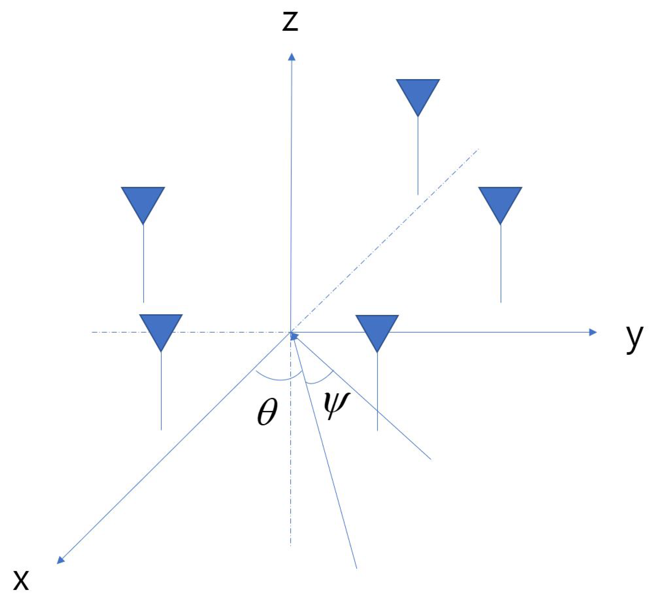
Consider the case of a uniform circular array (UCA) with M antenna elements. A signal is incident on the array and we are to estimate the azimuth angle and the elevation angle of the incident signal. Note that, for simultaneous estimation of the azimuth and elevation, the uniform linear array (ULA) cannot be adopted since ULA-based algorithm cannot uniquely estimate the azimuth and elevation due to the ambiguity pertinent to ULA structure.

Our interest in this paper is to get an closed-form expression of the MSEs of the azimuth and the elevation for the UCA geometry. In the interferometer algorithm for AOA estimation, the cost function in (2) is evaluated as the azimuth and the elevation vary, and the maximum value of the cost function can be evaluated. The azimuth and the elevation at which the maximum of the cost function occurs are chosen to be the azimuth estimate and the elevation estimate.

The UCA structure is adopted to simultaneously estimate the azimuth and the elevation of an incident signal, since the ULA structure is not able to simultaneously estimate the azimuth and the elevation of an incident signal due to an ambiguity problem.

If the array has identical responses to two different sets of DOA’s, then the ambiguity problem is said to arise. For the ULA, actually, there are infinitely many different sets of DOA’s resulting in identical responses, which makes the ULA inappropriate for simultaneous estimation of azimuth and elevation. On the other hand, for the UCA, no two different sets of DOA’s results in identical responses. Therefore, ambiguity problem does not occur for the UCA, which makes the UCA appropriate for simultaneous estimation of azimuth and elevation.

4. Performance Analysis of Phase Comparison Interferometer

In this paper, the analytic performance analysis of an interferometer algorithm for the UCA is considered. The UCA geometry is illustrated in Figure 1. The number of sensors in the UCA is equal to M.

Figure 1. This figure shows Uniform Circular Array (UCA). The two-dimensional array can simultaneously estimate azimuth and elevation of signal source.

The theoretical phase value of incident signal on the m-th sensor is expressed as

$${\varphi }_m=\frac{2\pi r}{\lambda }cos\left({\theta }^{\left(0\right)}-\frac{2\pi m}{M}\right)cos\left({\psi }^{\left(0\right)}\right)$$

(1)

In (1), ${\theta }^{\left(0\right)}$ and ${\psi }^{\left(0\right)}$ are true azimuth and true elevation, respectively. r is radius of circular array, $\lambda$ is wavelength, and M is the number of sensors.

For the UCA with $r=\frac{\lambda }{2}$, (1) reduces to

$${\varphi }_m=\pi cos\left({\theta }^{\left(0\right)}-\frac{2\pi m}{M}\right)cos\left({\psi }^{\left(0\right)}\right)$$

(2)

Since the product of two cosine functions varies from −1 to 1, the value in (2) varies from $-\pi$ to $\pi$, implying that there is no phase ambiguity for $r=\frac{\lambda }{2}$. If r is greater than $\frac{\lambda }{2}$, the value in (2) can be greater than $\pi$ or smaller than $-\pi$, implying that there is phase ambiguity for $r>\frac{\lambda }{2}$.

Phase measurement error is assumed to be a Gaussian random variables or uniform random variables with zero mean, and cosine cost function is used to derive correlation value between theoretical phase values and the estimated phase of the incident signal. Cosine cost function of interferometer algorithm is expressed as

$$J(\theta ,\psi )=\sum _{m=0}^{M-1}cos\left[\frac{2\pi r}{\lambda }cos(\theta -\frac{2\pi m}{M})cos\left(\psi \right)-{\widehat{\varphi }}_m\right]$$

(3)

where ${\widehat{\varphi }}_m$ is the measured phase of m-th sensor. In (3), $\theta$ and $\psi$ can be expressed as ${\theta }^{\left(0\right)}$ + $\Delta \theta$ and ${\psi }^{\left(0\right)}$ + $\Delta \psi$, respectively. Partial differentiations and linear approximation are used for optimization with respect to $\theta$ and $\psi$:

$${\left.\frac{\partial J\left(\theta ,\psi \right)}{\partial \theta }\right|}_{\begin{array}{c}\theta =\widehat{\theta }={\theta }^{\left(0\right)}+\Delta \theta \\ \psi =\widehat{\psi }={\psi }^{\left(0\right)}+\Delta \psi \end{array}}=\sum _{m=0}^{M-1}sin\left[\frac{2\pi r}{\lambda }cos(\theta -\frac{2\pi m}{M})cos\left(\psi \right)-{\widehat{\varphi }}_m\right]sin(\theta -\frac{2\pi m}{M})cos\left(\psi \right)=0.$$

(4)

$${\left.\frac{\partial J\left(\theta ,\psi \right)}{\partial \psi }\right|}_{\begin{array}{c}\theta =\widehat{\theta }={\theta }^{\left(0\right)}+\Delta \theta \\ \psi =\psi ={\psi }^{\left(0\right)}+\Delta \psi \end{array}}=\sum _{m=0}^{M-1}sin\left[\frac{2\pi r}{\lambda }cos(\theta -\frac{2\pi m}{M})cos\left(\psi \right)-{\widehat{\varphi }}_m\right]cos(\theta -\frac{2\pi m}{M})sin\left(\psi \right)=0.$$

(5)

Analytic MSE values of azimuth and elevation are derived by solving the simultaneous equations with respect to $\theta$ and $\psi$. Due to $sin\theta \approx \theta$ for small $\theta$, (4) can be rewritten as

$$\begin{array}{c}\hfill {\left.\frac{\partial J\left(\theta ,\psi \right)}{\partial \theta }\right|}_{\begin{array}{c}\theta =\widehat{\theta }={\theta }^{\left(0\right)}+\Delta \theta \\ \psi =\widehat{\psi }={\psi }^{\left(0\right)}+\Delta \psi \end{array}}=\sum _{m=0}^{M-1}\left[\frac{2\pi r}{\lambda }cos({\theta }^{\left(0\right)}+\Delta \theta -\frac{2\pi m}{M})cos({\psi }^{\left(0\right)}+\Delta \psi )-{\widehat{\varphi }}_m\right]sin({\theta }^{\left(0\right)}+\Delta \theta -\frac{2\pi m}{M})cos({\psi }^{\left(0\right)}+\Delta \psi )=0\end{array}$$

(6)

In (6), ${\theta }^{\left(0\right)}-\frac{2\pi m}{M}$ is replaced with $a_m$ and trigonometric identitiy is used:

$${\left.\frac{\partial J\left(\theta ,\psi \right)}{\partial \theta }\right|}_{\begin{array}{c}\theta =\widehat{\theta }={\theta }^{\left(0\right)}+\Delta \theta \\ \psi =\widehat{\psi }={\psi }^{\left(0\right)}+\Delta \psi \end{array}}=\sum _{m=0}^{M-1}\left[\frac{2\pi r}{\lambda }cos(a_m+\Delta \theta )cos({\psi }^{\left(0\right)}+\Delta \psi )-{\widehat{\varphi }}_m\right]sin(a_m+\Delta \theta )cos({\psi }^{\left(0\right)}+\Delta \psi )=0.$$

(7)

By distributive law, (7) can be rewritten as

$$\begin{array}{c}\hfill {\left.\frac{\partial J\left(\theta ,\psi \right)}{\partial \theta }\right|}_{\begin{array}{c}\theta =\widehat{\theta }={\theta }^{\left(0\right)}+\Delta \theta \\ \psi =\widehat{\psi }={\psi }^{\left(0\right)}+\Delta \psi \end{array}}=\sum _{m=0}^{M-1}\left[\frac{2\pi r}{\lambda }sin\left(2a_m+2\Delta \theta \right){cos}^2\left({\psi }^{\left(0\right)}+\Delta \psi \right)-{\widehat{\varphi }}_{m}sin(a_m+\Delta \theta )cos({\psi }^{\left(0\right)}+\Delta \psi )\right]=0.\end{array}$$

(8)

In Appendix B, it is shown why ${\displaystyle \sum _{m=0}^{M-1}}sin\left(2a_m+2\Delta \theta \right)$ is zero:

$${\left.\frac{\partial J\left(\theta ,\psi \right)}{\partial \theta }\right|}_{\begin{array}{c}\theta =\widehat{\theta }={\theta }^{\left(0\right)}+\Delta \theta \\ \psi =\widehat{\psi }={\psi }^{\left(0\right)}+\Delta \psi \end{array}}=\sum _{m=0}^{M-1}\left[\left({\varphi }_m+\Delta {\varphi }_m\right)sin(a_m+\Delta \theta )cos({\psi }^{\left(0\right)}+\Delta \psi )\right]=0.$$

(9)

Using $cos(\Delta \theta )\approx 1$, $sin(\Delta \theta )\approx \theta$, (9) can be rewritten as

$$\begin{array}{c}{\left.\frac{\partial J\left(\theta ,\psi \right)}{\partial \theta }\right|}_{\begin{array}{c}\theta =\widehat{\theta }={\theta }^{\left(0\right)}+\Delta \theta \\ \psi =\widehat{\psi }={\psi }^{\left(0\right)}+\Delta \psi \end{array}}={\displaystyle \sum _{m=0}^{M-1}}\left[\left({\varphi }_m+\Delta {\varphi }_m\right)sin(a_m+\Delta \theta )cos({\psi }^{\left(0\right)}+\Delta \psi )\right]\hfill \\ ={\displaystyle \sum _{m=0}^{M-1}}\left[\left({\varphi }_m+\Delta {\varphi }_m\right)\left(sin\left(a_m\right)+cos\left(a_m\right)\Delta \theta \right)\left(cos\left({\psi }^{\left(0\right)}\right)-sin\left({\psi }^{\left(0\right)}\right)\Delta \psi \right)\right]\hfill \\ ={\displaystyle \sum _{m=0}^{M-1}}\left[\begin{array}{c}\frac{2\pi r}{\lambda }cos\left(a_m\right)cos\left({\psi }^{\left(0\right)}\right)cos\left(a_m\right)\Delta \theta cos\left({\psi }^{\left(0\right)}\right)+\Delta {\varphi }_{m}sin\left(a_m\right)cos\left({\psi }^{\left(0\right)}\right)\hfill \\ -\Delta {\varphi }_{m}sin\left(a_m\right)sin\left({\psi }^{\left(0\right)}\right)\Delta \psi +\Delta {\varphi }_{m}cos\left(a_m\right)\Delta \theta cos\left({\psi }^{\left(0\right)}\right)\hfill \end{array}\right]=0.\hfill \end{array}$$

(10)

By using ${\displaystyle \sum _{m=0}^{M-1}}{cos}^2\left(a_m\right)={\displaystyle \sum _{m=0}^{M-1}}{sin}^2\left(a_m\right)=\frac{M}{2}$ which is derived in Appendix B, the right side of (10) is expressed as

$$\begin{array}{c}\Delta \theta \left[-\frac{2\pi r}{\lambda }\frac{M}{2}{\left\{cos\left({\psi }^{\left(0\right)}\right)\right\}}^2-cos\left({\psi }^{\left(0\right)}\right){\displaystyle \sum _{m=0}^{M-1}}\Delta {\varphi }_{m}cos\left(a_m\right)\right]+\Delta \psi \left[sin\left({\psi }^{\left(0\right)}\right){\displaystyle \sum _{m=0}^{M-1}}\Delta {\varphi }_{m}sin\left(a_m\right)\right]\\ =cos\left({\psi }^{\left(0\right)}\right){\displaystyle \sum _{m=0}^{M-1}}\Delta {\varphi }_{m}sin\left(a_m\right)\\ \end{array}$$

(11)

In Appendix A, the partial derivative of cost function with respect to the elevation is derived. Applying a few trigonometric identities to (A3) yields

$$\begin{array}{c}\Delta \theta \left[{\displaystyle \sum _{m=0}^{M-1}}\Delta {\varphi }_{m}sin\left(a_m\right)sin\left({\psi }^{\left(0\right)}\right)\right]+\Delta \psi \left[-\frac{2\pi r}{\lambda }\frac{M}{2}{\left\{sin\left({\psi }^{\left(0\right)}\right)\right\}}^2-cos\left({\psi }^{\left(0\right)}\right){\displaystyle \sum _{m=0}^{M-1}}\Delta {\varphi }_{m}cos\left(a_m\right))\right]\\ =sin\left({\psi }^{\left(0\right)}\right){\displaystyle \sum _{m=0}^{M-1}}\Delta {\varphi }_{m}cos\left(a_m\right)\\ \end{array}$$

(12)

From (11) and (12), $\Delta \theta$ and $\Delta \psi$ can be rewritten as

$$\Delta \theta =\frac{\left[\begin{array}{c}-\frac{2\pi r}{\lambda }\frac{M}{2}{\left\{sin\left({\psi }^{\left(0\right)}\right)\right\}}^{2}cos\left({\psi }^{\left(0\right)}\right){\displaystyle \sum _{m=0}^{M-1}}\Delta {\varphi }_{m}sin\left(a_m\right)\\ -\left[{\left\{cos\left({\psi }^{\left(0\right)}\right)\right\}}^2+cos\left({\psi }^{\left(0\right)}\right)sin\left({\psi }^{\left(0\right)}\right)\right]\\ ·\left\{{\displaystyle \sum _{m=0}^{M-1}}\Delta {\varphi }_{m}cos\left(a_m\right)\right\}\left\{{\displaystyle \sum _{m=0}^{M-1}}\Delta {\varphi }_{m}sin\left(a_m\right)\right\}\end{array}\right]}{\left[\begin{array}{c}{\left\{\frac{2\pi r}{\lambda }\frac{M}{2}\right\}}^2{\left\{sin\left({\psi }^{\left(0\right)}\right)\right\}}^2{\left\{cos\left({\psi }^{\left(0\right)}\right)\right\}}^2+\frac{2\pi r}{\lambda }\frac{M}{2}{\left\{cos\left({\psi }^{\left(0\right)}\right)\right\}}^3{\displaystyle \sum _{m=0}^{M-1}}\Delta {\varphi }_{m}cos\left(a_m\right)\\ +\frac{2\pi r}{\lambda }\frac{M}{2}{\left\{cos\left({\psi }^{\left(0\right)}\right)\right\}}^{2}sin\left({\psi }^{\left(0\right)}\right){\displaystyle \sum _{m=0}^{M-1}}\Delta {\varphi }_{m}cos\left(a_m\right)+{\left\{cos\left({\psi }^{\left(0\right)}\right){\displaystyle \sum _{m=0}^{M-1}}\Delta {\varphi }_{m}cos\left(a_m\right)\right\}}^2\\ -sin\left({\psi }^{\left(0\right)}\right)cos\left({\psi }^{\left(0\right)}\right)+·{\displaystyle \sum _{m=0}^{M-1}}\Delta {\varphi }_{m}sin\left(a_m\right){\displaystyle \sum _{m=0}^{M-1}}\Delta {\varphi }_{m}cos\left(a_m\right)\end{array}\right]}$$

(13)

$$\Delta \psi =\frac{\left[\begin{array}{c}-\frac{2\pi r}{\lambda }\frac{M}{2}sin\left({\psi }^{\left(0\right)}\right){\left\{cos\left({\psi }^{\left(0\right)}\right)\right\}}^2{\displaystyle \sum _{m=0}^{M-1}}\Delta {\varphi }_{m}cos\left(a_m\right)-\left[sin\left({\psi }^{\left(0\right)}\right)cos\left({\psi }^{\left(0\right)}\right)\right]\\ \left[{\left\{{\displaystyle \sum _{m=0}^{M-1}}\Delta {\varphi }_{m}cos\left(a_m\right)\right\}}^2+{\left\{{\displaystyle \sum _{m=0}^{M-1}}\Delta {\varphi }_{m}sin\left(a_m\right)\right\}}^2\right]\end{array}\right]}{\left[\begin{array}{c}{\left\{\frac{2\pi r}{\lambda }\frac{M}{2}\right\}}^2{\left\{sin\left({\psi }^{\left(0\right)}\right)\right\}}^2{\left\{cos\left({\psi }^{\left(0\right)}\right)\right\}}^2+\frac{2\pi r}{\lambda }\frac{M}{2}{\left\{cos\left({\psi }^{\left(0\right)}\right)\right\}}^3{\displaystyle \sum _{m=0}^{M-1}}\Delta {\varphi }_{m}cos\left(a_m\right)\hfill \\ +\frac{2\pi r}{\lambda }\frac{M}{2}{\left\{cos\left({\psi }^{\left(0\right)}\right)\right\}}^{2}sin\left({\psi }^{\left(0\right)}\right){\displaystyle \sum _{m=0}^{M-1}}\Delta {\varphi }_{m}cos\left(a_m\right)+{\left\{cos\left({\psi }^{\left(0\right)}\right){\displaystyle \sum _{m=0}^{M-1}}\Delta {\varphi }_{m}cos\left(a_m\right)\right\}}^2\hfill \\ -sin\left({\psi }^{\left(0\right)}\right)cos\left({\psi }^{\left(0\right)}\right)·{\displaystyle \sum _{m=0}^{M-1}}\Delta {\varphi }_{m}sin\left(a_m\right){\displaystyle \sum _{m=0}^{M-1}}\Delta {\varphi }_{m}cos\left(a_m\right)\hfill \end{array}\right]}$$

(14)

Since $-\frac{2\pi r}{\lambda }\frac{M}{2}{\left\{sin\left({\psi }^{\left(0\right)}\right)\right\}}^{2}cos\left({\psi }^{\left(0\right)}\right){\displaystyle \sum _{m=0}^{M-1}}\Delta {\varphi }_{m}sin\left(a_m\right)$ in the numerator of (13) and ${\left\{\frac{2\pi r}{\lambda }\frac{M}{2}\right\}}^2{\left\{sin\left({\psi }^{\left(0\right)}\right)\right\}}^2{\left\{cos\left({\psi }^{\left(0\right)}\right)\right\}}^2$ in the denominator of (13) is larger than other terms, (13) and (14) can be approximated as

$$\Delta \theta =\frac{-\frac{2\pi r}{\lambda }\frac{M}{2}{\left\{sin\left({\psi }^{\left(0\right)}\right)\right\}}^{2}cos\left({\psi }^{\left(0\right)}\right){\displaystyle \sum _{m=0}^{M-1}}\Delta {\varphi }_{m}sin\left(a_m\right)}{{\left\{\frac{2\pi r}{\lambda }\frac{M}{2}\right\}}^2{\left\{sin\left({\psi }^{\left(0\right)}\right)\right\}}^2{\left\{cos\left({\psi }^{\left(0\right)}\right)\right\}}^2}$$

(15)

$$\Delta \psi =\frac{-\frac{2\pi r}{\lambda }\frac{M}{2}sin\left({\psi }^{\left(0\right)}\right){\left\{cos\left({\psi }^{\left(0\right)}\right)\right\}}^2{\displaystyle \sum _{m=0}^{M-1}}\Delta {\varphi }_{m}cos\left(a_m\right)}{{\left\{\frac{2\pi r}{\lambda }\frac{M}{2}\right\}}^2{\left\{sin\left({\psi }^{\left(0\right)}\right)\right\}}^2{\left\{cos\left({\psi }^{\left(0\right)}\right)\right\}}^2}.$$

(16)

Since the phase errors in the different sensors are uncorrelated, we have

$$\begin{array}{c}E\left[{\left\{{\displaystyle \sum _{m=0}^{M-1}}\Delta {\phi }_{m}sin\left(a_m\right)\right\}}^2\right]={\sigma }_{\varphi }^2\frac{M}{2}\hfill \\ E\left[{\left\{{\displaystyle \sum _{m=0}^{M-1}}\Delta {\phi }_{m}cos\left(a_m\right)\right\}}^2\right]={\sigma }_{\varphi }^2\frac{M}{2}.\hfill \end{array}$$

(17)

(17) is derived in Appendix C.

Applying the first equation of (17) to (15), the azimuth MSE can be written as

$$E\left[{(\Delta \theta )}^2\right]={\left[\frac{-\frac{2\pi r}{\lambda }\frac{M}{2}{\left\{sin\left({\psi }^{\left(0\right)}\right)\right\}}^{2}cos\left({\psi }^{\left(0\right)}\right)}{{\left\{\frac{2\pi r}{\lambda }\frac{M}{2}\right\}}^2{\left\{sin\left({\psi }^{\left(0\right)}\right)\right\}}^2{\left\{cos\left({\psi }^{\left(0\right)}\right)\right\}}^2}\right]}^{2}E\left[{\left({\displaystyle \sum _{m=0}^{M-1}}\Delta {\varphi }_{m}sin\left(a_m\right)\right)}^2\right]=\frac{{\sigma }_{\phi }^2}{\frac{M}{2}{\left\{\frac{2\pi r}{\lambda }\right\}}^2{\left\{cos\left({\psi }^{\left(0\right)}\right)\right\}}^2}.$$

(18)

Similarly, applyting the second equation of (17) to (16), the elevation MSE can be expressed as

$$E\left[{(\Delta \psi )}^2\right]={\left[\frac{-\frac{2\pi r}{\lambda }\frac{M}{2}{\left\{sin\left({\psi }^{\left(0\right)}\right)\right\}}^{2}cos\left({\psi }^{\left(0\right)}\right)}{{\left\{\frac{2\pi r}{\lambda }\frac{M}{2}\right\}}^2{\left\{sin\left({\psi }^{\left(0\right)}\right)\right\}}^2{\left\{cos\left({\psi }^{\left(0\right)}\right)\right\}}^2}\right]}^{2}E\left[{\left({\displaystyle \sum _{m=0}^{M-1}}\Delta {\varphi }_{m}cos\left(a_m\right)\right)}^2\right]=\frac{{\sigma }_{\phi }^2}{\frac{M}{2}{\left\{\frac{2\pi r}{\lambda }\right\}}^2{\left\{sin\left({\psi }^{\left(0\right)}\right)\right\}}^2}.$$

(19)

From (18) and (19), for small $\psi$, $E\left[{(\Delta \psi )}^2\right]$ is much greater than $E\left[{(\Delta \theta )}^2\right]$. That is, for a signal with small incident elevation, elevation error is much larger than the azimuth error. This could be confirmed by simulation in [13].

We are concerned with how the azimuth MSE is dependent on the true azimuth or the true elevation. In addition, the dependence of the elevation MSE on the true azimuth or the true elevation should be addressed.

From (18), the azimuth MSE only depends on the true elevation, not on the true azimuth. From (19), the elevation MSE is also dependent on the true elevation, not on the true azimuth.

Although both the azimuth MSE and the elevation MSE are dependent on the true elevation, not on the true azimuth, how the azimuth MSE varies with the increase of the true elevation is different from how the elevation MSE varies with the increase of the true elevation. The azimuth MSE increases with the increase of the true elevation. On the other hand, the elevation MSE decreases with the increase of the true elevation.

5. Equivalent Derivation of the MSE of Azimuth and the MSE of Elevation

In this section, another way to obtain (18) and (19) is described. The theoretical phase value on the m-th sensor for an incident signal from azimuth, $\theta$, and elevation, $\psi$, can be written as

$${\varphi }_m=\frac{2\pi r}{\lambda }cos\left(\theta -\frac{2\pi m}{M}\right)cos\left(\psi \right)$$

(20)

Explicit expressions of $\frac{\partial {\varphi }_m}{\partial \theta }$ and $\frac{\partial {\varphi }_m}{\partial \psi }$ can be obtained from partial differentiations of (20) with respect to $\theta$ and $\psi$ :

$$\frac{\partial {\varphi }_m}{\partial \theta }=-\frac{2\pi r}{\lambda }sin\left(\theta -\frac{2\pi m}{M}\right)cos\left(\psi \right)$$

(21)

$$\frac{\partial {\varphi }_m}{\partial \psi }=-\frac{2\pi r}{\lambda }cos\left(\theta -\frac{2\pi m}{M}\right)sin\left(\psi \right)$$

(22)

Perturbation in ${\varphi }_m$ due to small change in $\theta$ and $\psi$ can be formulated as

$$\Delta {\varphi }_m=\frac{\partial {\varphi }_m}{\partial \theta }\Delta \theta +\frac{\partial {\varphi }_m}{\partial \psi }\Delta \psi$$

(23)

Note that (23) is equivalent to the first-order Taylor series expansion. (23) can be written in matrix form as follows :

$$\left[\begin{array}{c}\Delta {\varphi }_1\\ \Delta {\varphi }_2\\ ⋮\\ \Delta {\varphi }_M\end{array}\right]=\left[\begin{array}{c}\frac{\partial {\varphi }_1}{\partial \theta }\\ \frac{\partial {\varphi }_2}{\partial \theta }\\ ⋮\\ \frac{\partial {\varphi }_M}{\partial \theta }\end{array}\begin{array}{c}\frac{\partial {\varphi }_1}{\partial \psi }\\ \frac{\partial {\varphi }_2}{\partial \psi }\\ ⋮\\ \frac{\partial {\varphi }_M}{\partial \psi }\end{array}\right]\left[\begin{array}{c}\Delta \theta \hfill \\ \Delta \psi \hfill \end{array}\right]$$

(24)

Let $\mathbf{A}$ and $\mathbf{b}$ defined as

$$\mathbf{A}\equiv \left[\begin{array}{c}\frac{\partial {\varphi }_0}{\partial \theta }\\ \frac{\partial {\varphi }_1}{\partial \theta }\\ ⋮\\ \frac{\partial {\varphi }_{M-1}}{\partial \theta }\end{array}\begin{array}{c}\frac{\partial {\varphi }_0}{\partial \psi }\\ \frac{\partial {\varphi }_1}{\partial \psi }\\ ⋮\\ \frac{\partial {\varphi }_{M-1}}{\partial \psi }\end{array}\right]$$

(25)

$$\mathbf{b}=\left[\begin{array}{c}\Delta {\varphi }_0\\ \Delta {\varphi }_1\\ ⋮\\ \Delta {\varphi }_{M-1}\end{array}\right]$$

(26)

By substituting (21) and (22) in (25), $\mathbf{A}$ can be explicitly written as

$$\mathbf{A}\equiv -\frac{2\pi r}{\lambda }\left[\begin{array}{c}sin\left(\theta \right)cos\left(\psi \right)\\ sin\left(\theta -\frac{2\pi }{M}\right)cos\left(\psi \right)\\ ⋮\\ sin\left(\theta -\frac{2\pi \left(M-1\right)}{M}\right)cos\left(\psi \right)\end{array}\begin{array}{c}cos\left(\theta \right)sin\left(\psi \right)\\ cos\left(\theta -\frac{2\pi }{M}\right)sin\left(\psi \right)\\ ⋮\\ cos\left(\theta -\frac{2\pi \left(M-1\right)}{M}\right)sin\left(\psi \right)\end{array}\right].$$

(27)

In terms of $\mathbf{A}$ and $\mathbf{b}$, (24) can be expressed as

$$\mathbf{b}=\mathbf{A}\left[\begin{array}{c}\Delta \theta \hfill \\ \Delta \psi \hfill \end{array}\right].$$

(28)

$\mathbf{A}$ defined in (25) is not a square matrix. Therefore, it is not invertible. Since (28) is an overdetermined system, the least squares approach can be adopted to get ${\left[\begin{array}{cc}\Delta \theta & \Delta \psi \end{array}\right]}^T$ from (28):

$$\left[\begin{array}{c}\Delta \theta \hfill \\ \Delta \psi \hfill \end{array}\right]={\left({\mathbf{A}}^T\mathbf{A}\right)}^{-1}\left({\mathbf{A}}^T\mathbf{b}\right).$$

(29)

By tranposing (29), $\left[\begin{array}{cc}\Delta \theta & \Delta \psi \end{array}\right]$ can be written as

$$\left[\begin{array}{cc}\Delta \theta & \Delta \psi \end{array}\right]={\mathbf{b}}^T\mathbf{A}{\left({\mathbf{AA}}^T\right)}^{-1}.$$

(30)

From (29) and (30), we have

$$\left[\begin{array}{c}\Delta \theta \hfill \\ \Delta \psi \hfill \end{array}\right]\left[\Delta \theta \Delta \psi \right]=\left[\begin{array}{cc}\Delta {\theta }^2& \Delta \theta \Delta \psi \\ \Delta \psi \Delta \theta & \Delta {\psi }^2\end{array}\right]={\left({\mathbf{A}}^T\mathbf{A}\right)}^{-1}{\mathbf{A}}^T{\mathbf{bb}}^T\mathbf{A}{\left({\mathbf{AA}}^T\right)}^{-1}.$$

(31)

An additive noise on each sensor location is spatially white. From uncorrelatedness of $\Delta {\varphi }_m$, we have

$$E\left[\Delta {\varphi }_m\Delta {\varphi }_n\right]=\left\{\begin{array}{c}E\left[\Delta {\varphi }_m^2\right]={\sigma }_{\varphi }^{2}m=n\\ E\left[\Delta {\varphi }_m\right]E\left[\Delta {\varphi }_n\right]=0m\ne n\end{array}\right.$$

(32)

where $E\left[\Delta {\varphi }_m\right]=0$ and $E\left[\Delta {\varphi }_n\right]=0$ are used both for $m=n$ and for $m\ne n$. $E\left[\Delta {\varphi }_m\right]=0$ and $E\left[\Delta {\varphi }_n\right]=0$ are valid when $\Delta {\varphi }_m$ and $\Delta {\varphi }_n$ are zero-mean random variables.

From (26), ${\mathbf{bb}}^{\mathbf{T}}$ can be expressed as

$${\mathbf{bb}}^T=\left[\begin{array}{c}\Delta {\varphi }_0\\ \Delta {\varphi }_2\\ ⋮\\ \Delta {\varphi }_{M-1}\end{array}\right]\left[\begin{array}{cccc}\Delta {\varphi }_0& \Delta {\varphi }_1& \cdots & \Delta {\varphi }_{M-1}\end{array}\right]=\left[\begin{array}{cccc}\Delta {\varphi }_0^2& \Delta {\varphi }_0\Delta {\varphi }_1& \cdots & \Delta {\varphi }_0\Delta {\varphi }_{M-1}\\ \Delta {\varphi }_1\Delta {\varphi }_0& \Delta {\varphi }_1^2& \cdots & \Delta {\varphi }_1\Delta {\varphi }_{M-1}\\ ⋮& ⋮& \ddots & ⋮\\ \Delta {\varphi }_{M-1}\Delta {\varphi }_0& \Delta {\varphi }_{M-1}\Delta {\varphi }_1& \cdots & \Delta {\varphi }_{M-1}^2\end{array}\right].$$

(33)

From (33), the expected value of ${\mathbf{bb}}^{\mathbf{T}}$, $E\left[{\mathbf{bb}}^{\mathbf{T}}\right]$, can be written as

$$E\left[{\mathbf{bb}}^{\mathbf{T}}\right]=\left[\begin{array}{cccc}E\left[\Delta {\varphi }_0^2\right]& E\left[\Delta {\varphi }_0\Delta {\varphi }_1\right]& \cdots & E\left[\Delta {\varphi }_0\Delta {\varphi }_{M-1}\right]\\ E\left[\Delta {\varphi }_1\Delta {\varphi }_0\right]& E\left[\Delta {\varphi }_1^2\right]& \cdots & E\left[\Delta {\varphi }_1\Delta {\varphi }_{M-1}\right]\\ ⋮& ⋮& \ddots & ⋮\\ E\left[\Delta {\varphi }_{M-1}\Delta {\varphi }_0\right]& E\left[\Delta {\varphi }_{M-1}\Delta {\varphi }_1\right]& \cdots & E\left[\Delta {\varphi }_{M-1}^2\right]\end{array}\right].$$

(34)

By substituting (32) in (34), $E\left[{\mathbf{bb}}^{\mathbf{T}}\right]$ can be simplified to

$$E\left[{\mathbf{bb}}^{\mathbf{T}}\right]=\left[\begin{array}{cccc}{\sigma }_{\varphi }^2& 0& \cdots & 0\\ 0& {\sigma }_{\varphi }^2& \cdots & 0\\ ⋮& ⋮& \ddots & ⋮\\ 0& 0& \cdots & {\sigma }_{\varphi }^2\end{array}\right]={\sigma }_{\varphi }^2{\mathbf{I}}_M.$$

(35)

where ${\mathbf{I}}_M$ denotes an $M\times M$ identity matrix. From (31), covariance matrix can be expressed as

$$\left[\begin{array}{cc}E\left[\Delta {\theta }^2\right]& E\left[\Delta \theta \Delta \psi \right]\\ E\left[\Delta \theta \Delta \psi \right]& E\left[\Delta {\psi }^2\right]\end{array}\right]=E\left[{\left({\mathbf{A}}^T\mathbf{A}\right)}^{-1}{\mathbf{A}}^T{\mathbf{bb}}^T\mathbf{A}{\left({\mathbf{AA}}^T\right)}^{-1}\right].$$

(36)

Since $\mathbf{A}$ in (27) is not stochastic, (36) can be reduced to

$$\left[\begin{array}{cc}E\left[\Delta {\theta }^2\right]& E\left[\Delta \theta \Delta \psi \right]\\ E\left[\Delta \theta \Delta \psi \right]& E\left[\Delta {\psi }^2\right]\end{array}\right]={\left({\mathbf{A}}^T\mathbf{A}\right)}^{-1}{\mathbf{A}}^{T}E\left[{\mathbf{bb}}^T\right]\mathbf{A}{\left({\mathbf{AA}}^T\right)}^{-1}.$$

(37)

Substituting (35) in (37), we have

$$\left[\begin{array}{cc}E\left[\Delta {\theta }^2\right]& E\left[\Delta \theta \Delta \psi \right]\\ E\left[\Delta \theta \Delta \psi \right]& E\left[\Delta {\psi }^2\right]\end{array}\right]={\sigma }_{\varphi }^2{\left({\mathbf{A}}^T\mathbf{A}\right)}^{-1}{\mathbf{A}}^T\mathbf{A}{\left({\mathbf{AA}}^T\right)}^{-1}={\sigma }_{\varphi }^2{\left({\mathbf{A}}^T\mathbf{A}\right)}^{-1}\left({\mathbf{A}}^T\mathbf{A}\right){\left({\mathbf{AA}}^T\right)}^{-1}={\sigma }_{\varphi }^2{\left({\mathbf{A}}^T\mathbf{A}\right)}^{-1}.$$

(38)

From (27), ${\mathbf{A}}^T\mathbf{A}$ is given by

$$\begin{array}{c}\hfill \begin{array}{c}{\mathbf{A}}^T\mathbf{A}={\left(\frac{2\pi r}{\lambda }\right)}^2\left[\begin{array}{cc}{cos}^2\left(\psi \right){\displaystyle \sum _{m=0}^{M-1}}{sin}^2\left(\theta -\frac{2\pi m}{M}\right)& cos\left(\psi \right)sin\left(\psi \right){\displaystyle \sum _{m=0}^{M-1}}sin\left(\theta -\frac{2\pi m}{M}\right)cos\left(\theta -\frac{2\pi m}{M}\right)\\ sin\left(\psi \right)cos\left(\psi \right){\displaystyle \sum _{m=0}^{M-1}}cos\left(\theta -\frac{2\pi m}{M}\right)sin\left(\theta -\frac{2\pi m}{M}\right)& {sin}^2\left(\psi \right){\displaystyle \sum _{m=0}^{M-1}}{cos}^2\left(\theta -\frac{2\pi m}{M}\right)\end{array}\right]\hfill \\ ={\left(\frac{2\pi r}{\lambda }\right)}^2\left[\begin{array}{cc}{cos}^2\left(\psi \right){\displaystyle \sum _{m=0}^{M-1}}{sin}^2\left(\theta -\frac{2\pi m}{M}\right)& \frac{1}{2}cos\left(\psi \right)sin\left(\psi \right){\displaystyle \sum _{m=0}^{M-1}}sin\left(2\theta -\frac{4\pi m}{M}\right)\\ \frac{1}{2}sin\left(\psi \right)cos\left(\psi \right){\displaystyle \sum _{m=0}^{M-1}}sin\left(2\theta -\frac{4\pi m}{M}\right)& {sin}^2\left(\psi \right){\displaystyle \sum _{m=0}^{M-1}}{cos}^2\left(\theta -\frac{2\pi m}{M}\right)\end{array}\right].\hfill \end{array}\end{array}$$

(39)

In Appendix B, the following identities have been derived:

$${\displaystyle \sum _{m=0}^{M-1}}{sin}^2\left(\theta -\frac{2\pi m}{M}\right)=\frac{M}{2}$$

(40)

$${\displaystyle \sum _{m=0}^{M-1}}{cos}^2\left(\theta -\frac{2\pi m}{M}\right)=\frac{M}{2}$$

(41)

$${\displaystyle \sum _{m=0}^{M-1}}sin\left(2\theta -\frac{4\pi m}{M}\right)=0.$$

(42)

By substituting (40)–(42) in (39), ${\mathbf{A}}^T\mathbf{A}$ can be reduced to

$${\mathbf{A}}^T\mathbf{A}={\left(\frac{2\pi r}{\lambda }\right)}^2\left[\begin{array}{cc}\frac{M}{2}{\left\{cos\left(\psi \right)\right\}}^2& 0\\ 0& \frac{M}{2}{\left\{sin\left(\psi \right)\right\}}^2\end{array}\right]=\frac{M}{2}{\left(\frac{2\pi r}{\lambda }\right)}^2\left[\begin{array}{cc}{\left\{cos\left(\psi \right)\right\}}^2& 0\\ 0& {\left\{sin\left(\psi \right)\right\}}^2\end{array}\right].$$

(43)

Since ${\mathbf{A}}^T\mathbf{A}$ is a diagonal matrix, ${\left({\mathbf{A}}^T\mathbf{A}\right)}^{-1}$ is also a diagonal matrix. The diagonal entries of ${\left({\mathbf{A}}^T\mathbf{A}\right)}^{-1}$ are given by the reciprocals of the diagonal entries of ${\mathbf{A}}^T\mathbf{A}$:

$${\left({\mathbf{A}}^T\mathbf{A}\right)}^{-1}=\frac{1}{\frac{M}{2}{\left(\frac{2\pi r}{\lambda }\right)}^2}\left[\begin{array}{cc}\frac{1}{{\left\{cos\left(\psi \right)\right\}}^2}& 0\\ 0& \frac{1}{{\left\{sin\left(\psi \right)\right\}}^2}\end{array}\right].$$

(44)

By substituting (44) in (38), the covariance matrix can be expressed as :

$$\left[\begin{array}{cc}E\left[\Delta {\theta }^2\right]& E\left[\Delta \theta \Delta \psi \right]\\ E\left[\Delta \theta \Delta \psi \right]& E\left[\Delta {\psi }^2\right]\end{array}\right]=\frac{{\sigma }_{\varphi }^2}{\frac{M}{2}{\left(\frac{2\pi r}{\lambda }\right)}^2}\left[\begin{array}{cc}\frac{1}{{\left\{cos\left(\psi \right)\right\}}^2}& 0\\ 0& \frac{1}{{\left\{sin\left(\psi \right)\right\}}^2}\end{array}\right].$$

(45)

6. Numerical Results

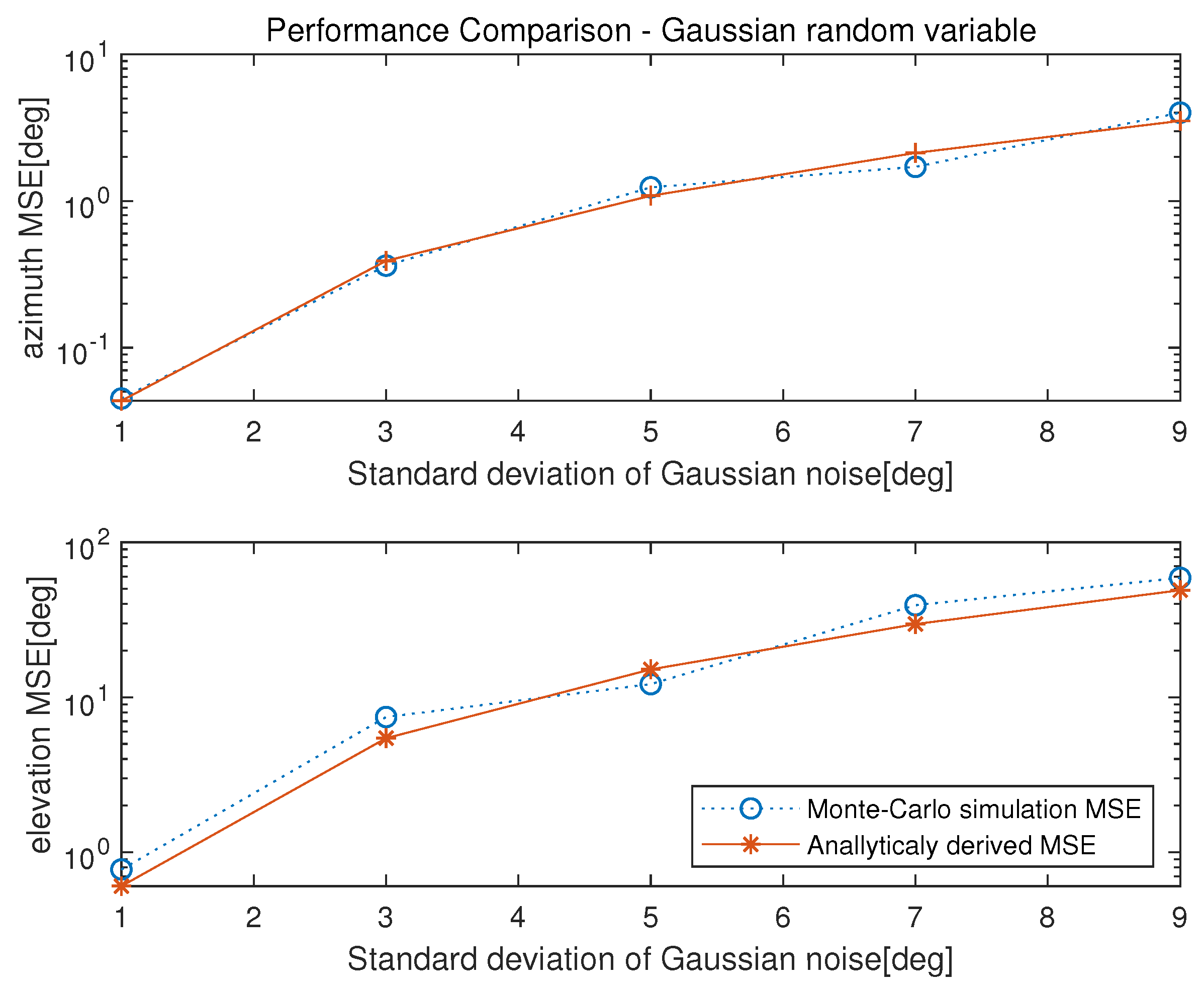
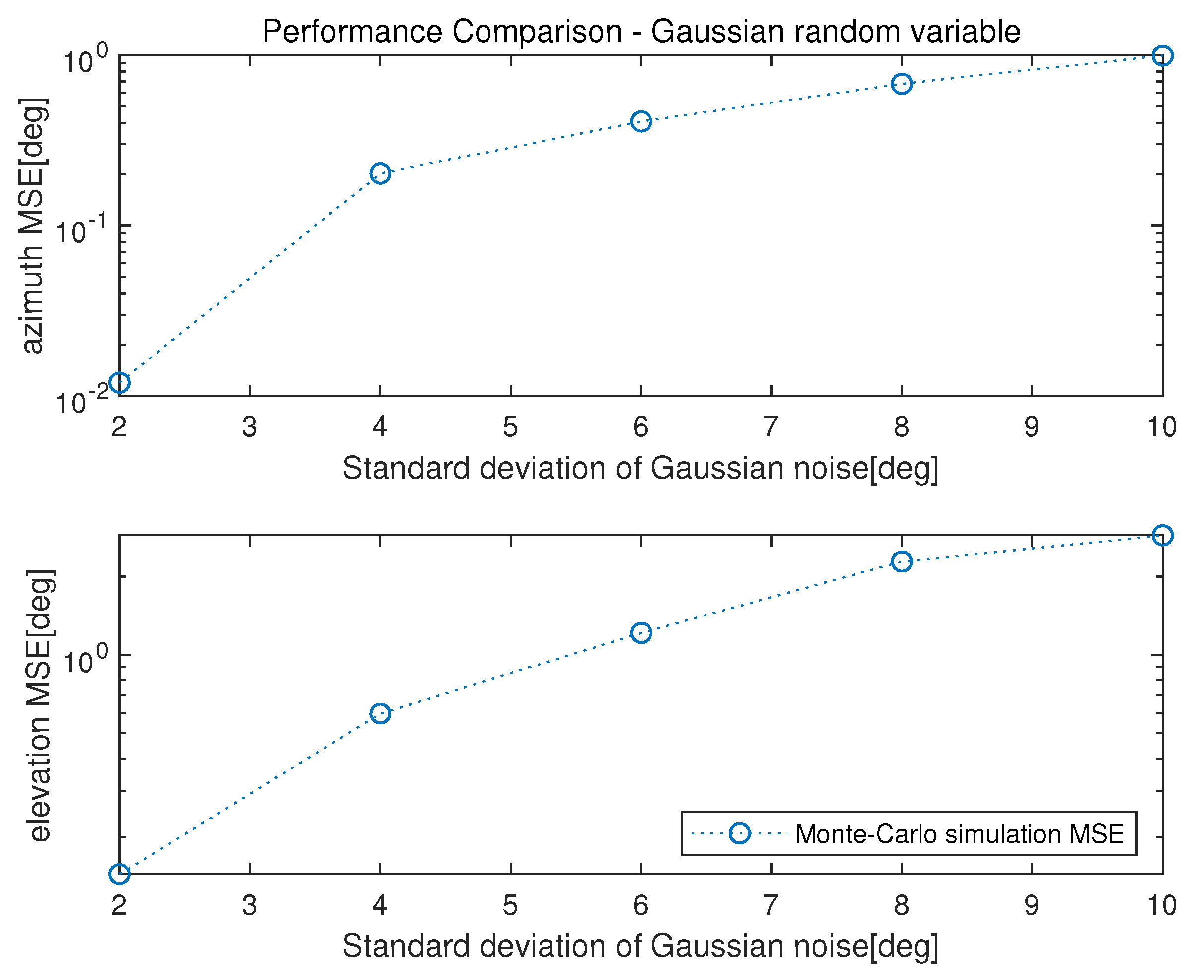
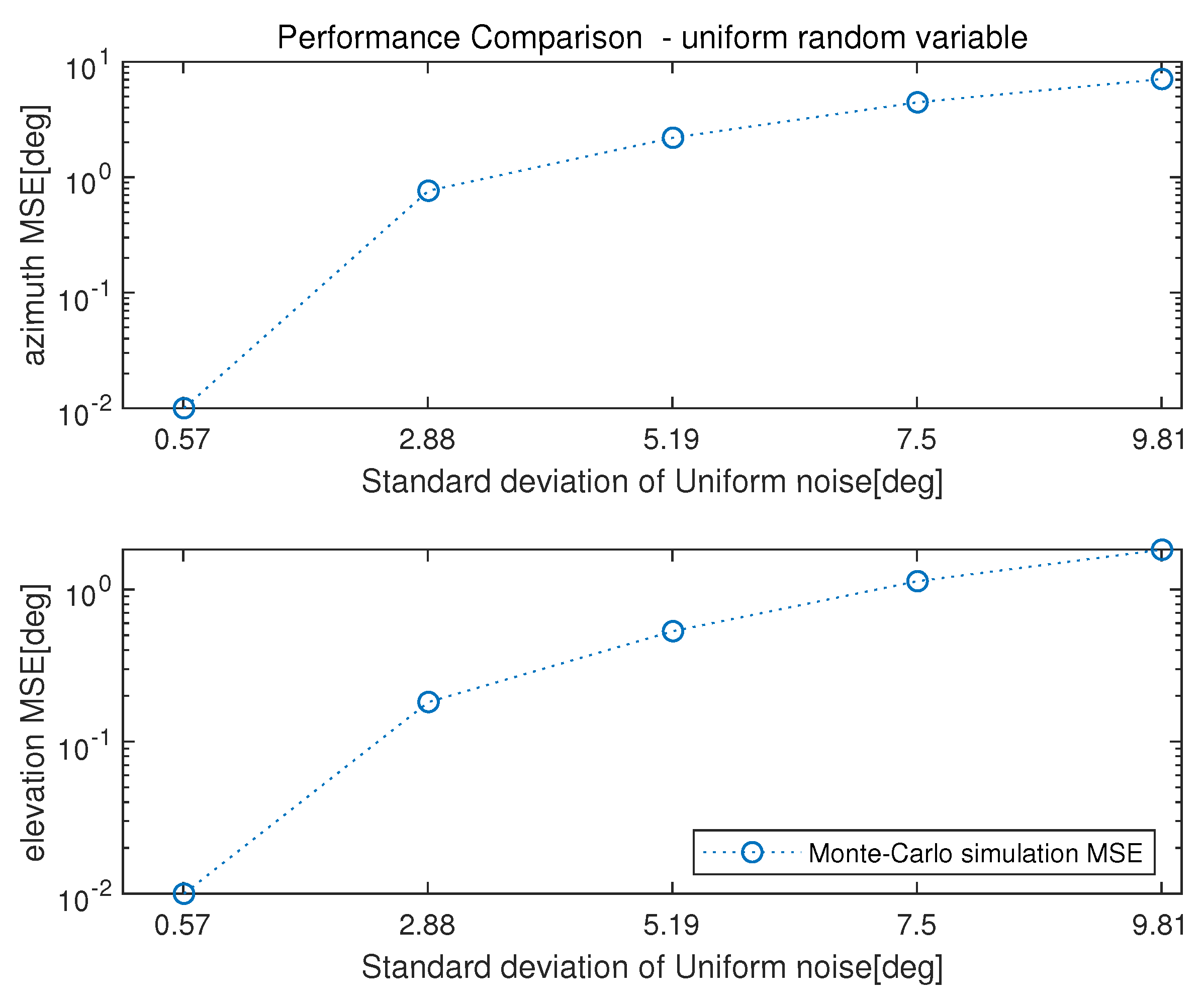
In this section, a computer simulation was conducted on the MATLAB R2017a version. The simulation environment is set as shown in Table 1. The phase error is assumed to be a Gaussian or a uniform random variables. We compared the MSE of the Monte Carlo simulation for various values of measurement noise variance. The x-axis of the Figure represents the standard deviation, and the y-axis represents the MSE value on a log scale. The simulation was performed by fixing the azimuth angle to 120 degrees and changing the elevation angle to 15${}^{°}$, 45${}^{°}$, and 75${}^{°}$.

Table 1. Simulation condition.

Parameter	Value
Number of sensors	5
Array architecture	Uniform Circular Array
Monte-Carlo iteration	1000
Radius of array	0.5$\lambda$

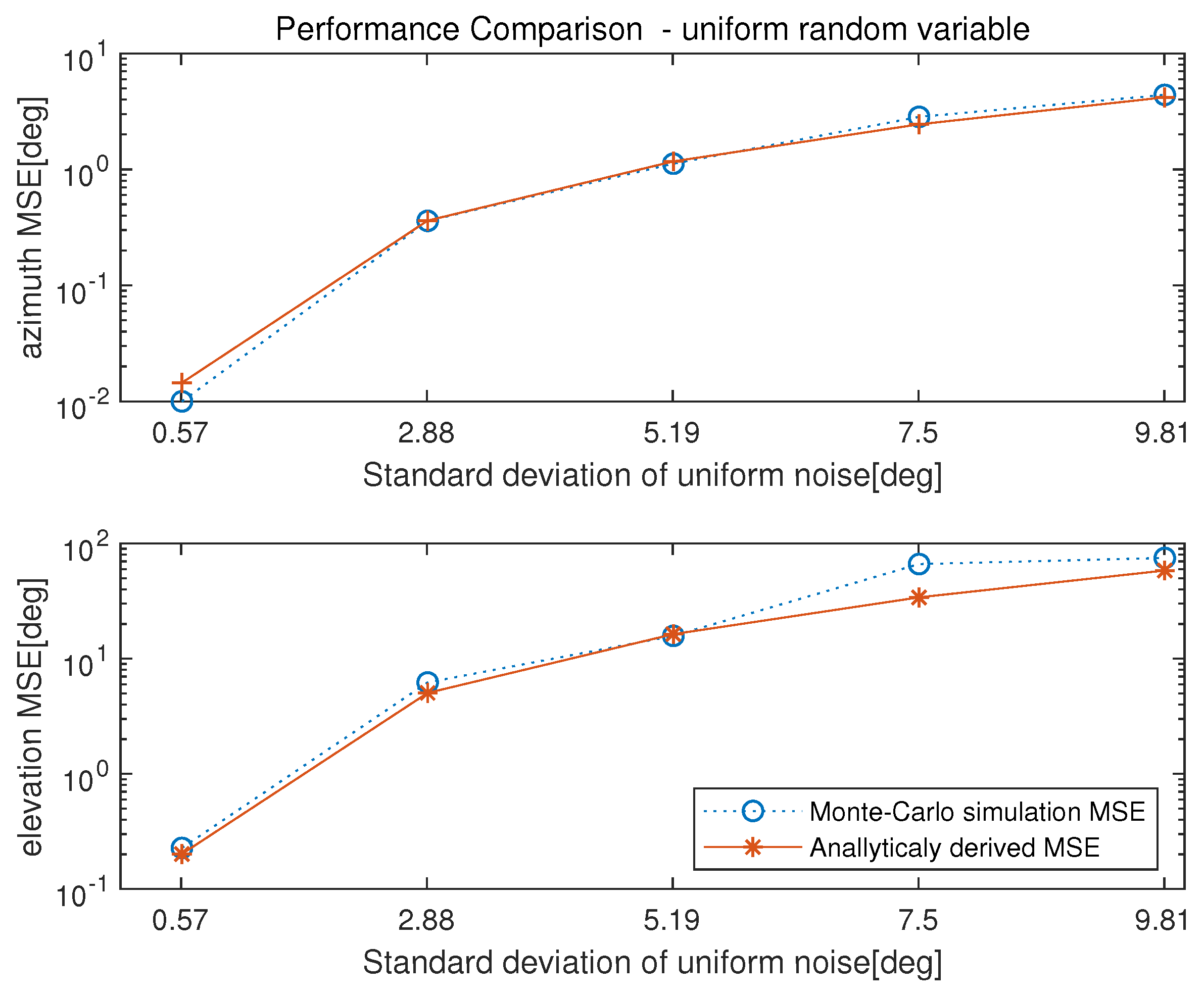
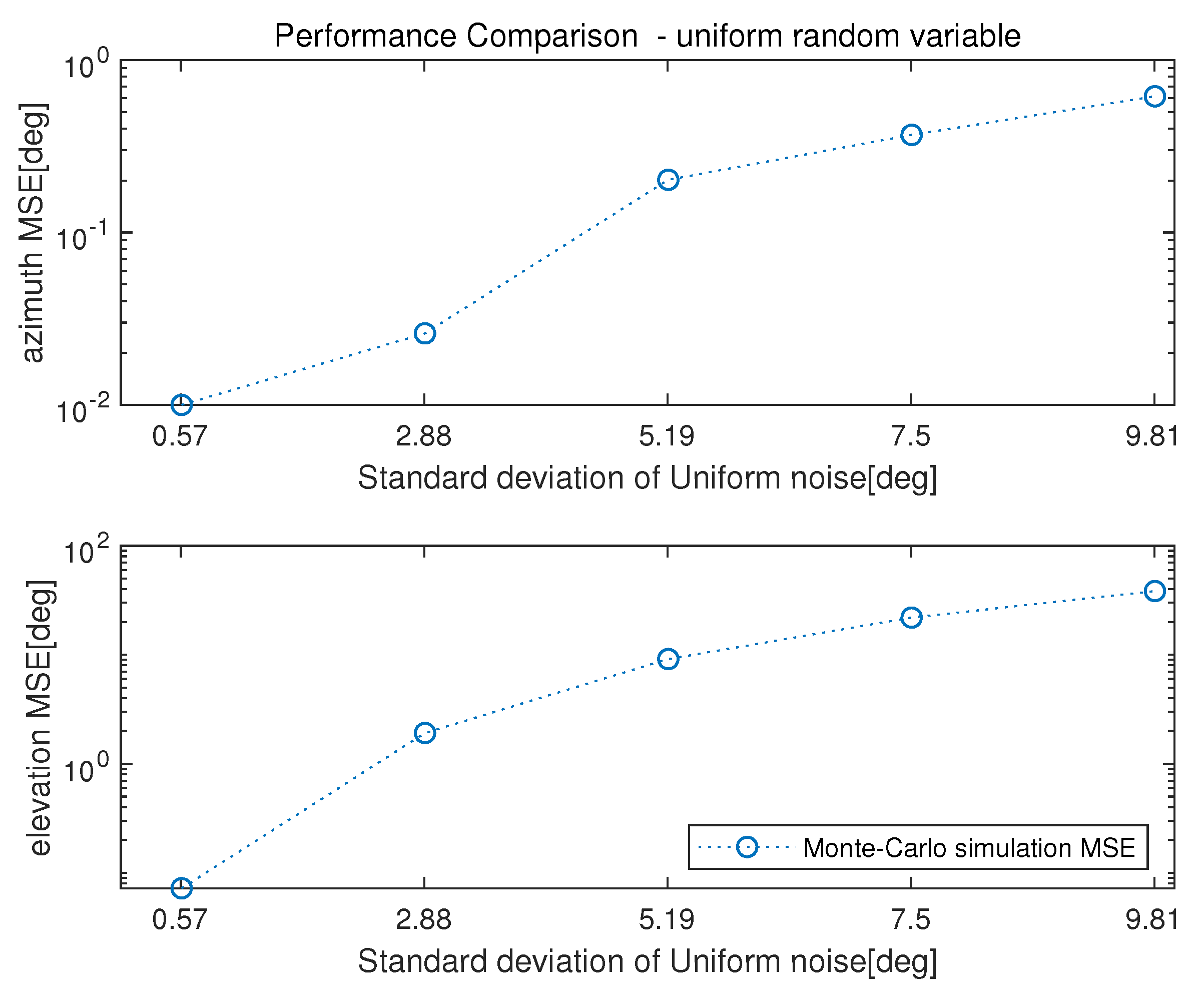
The noise of the phase is assumed to be the zero-mean uniform random variables. Since the random variables are assumed to be uniformly distributed between $-A$ degrees and A degrees, standard deviation of uniform random variables is $\sigma =\sqrt{\frac{A^2}{3}}$. Since A values are 1${}^{°}$, 5${}^{°}$, 9${}^{°}$, 13${}^{°}$ and 17${}^{°}$, standard deviations are 0.57${}^{°}$, 2.88${}^{°}$, 5.19${}^{°}$, 7.5${}^{°}$ and 9.81${}^{°}$, respectively.

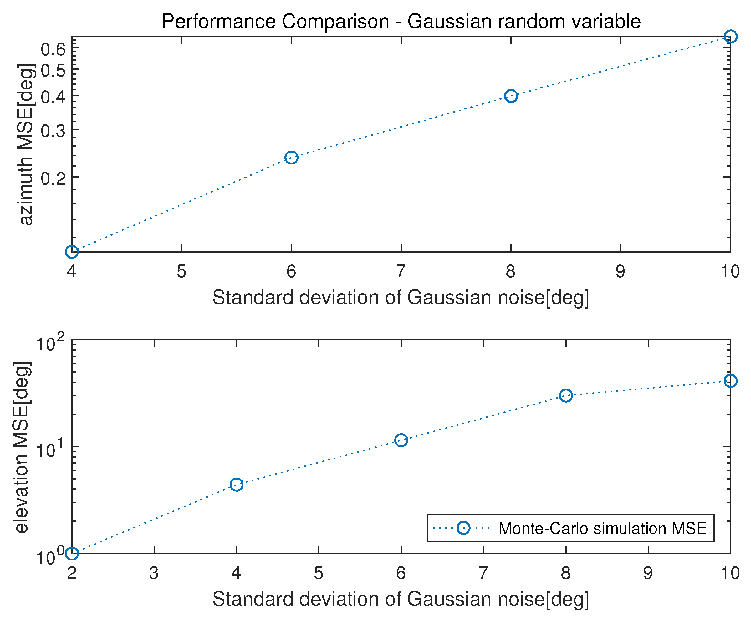
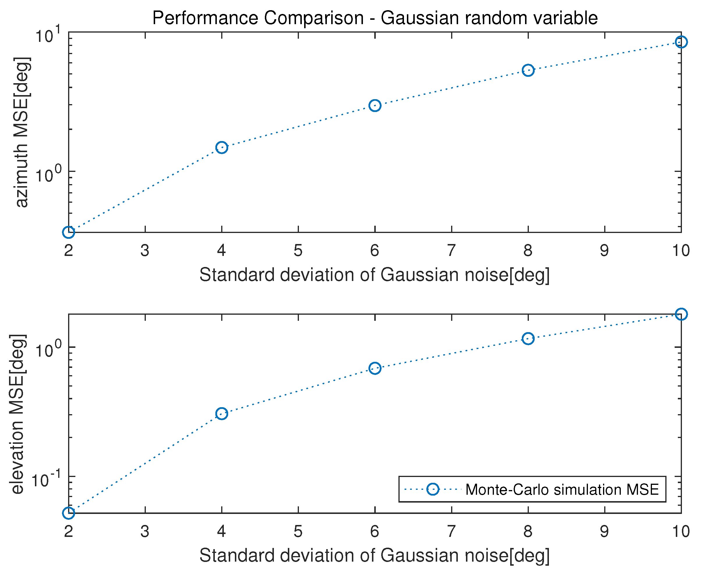
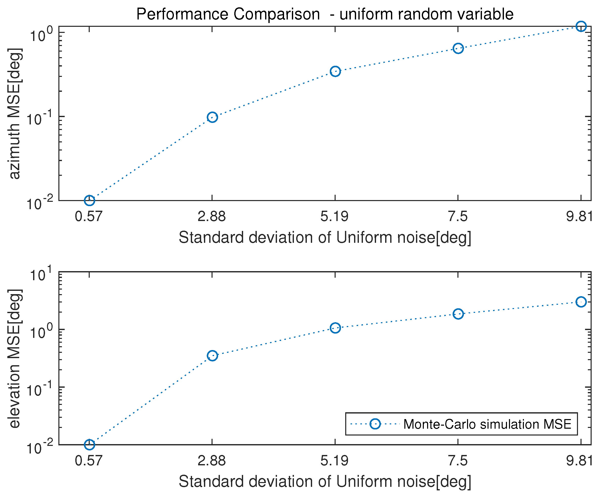
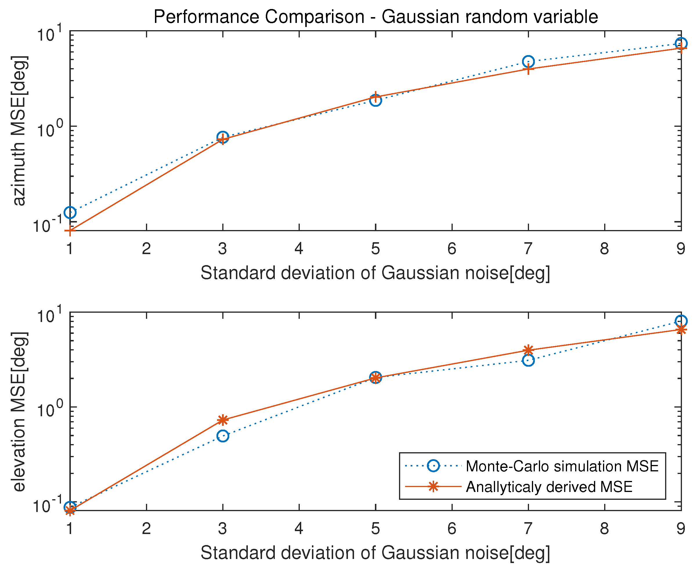
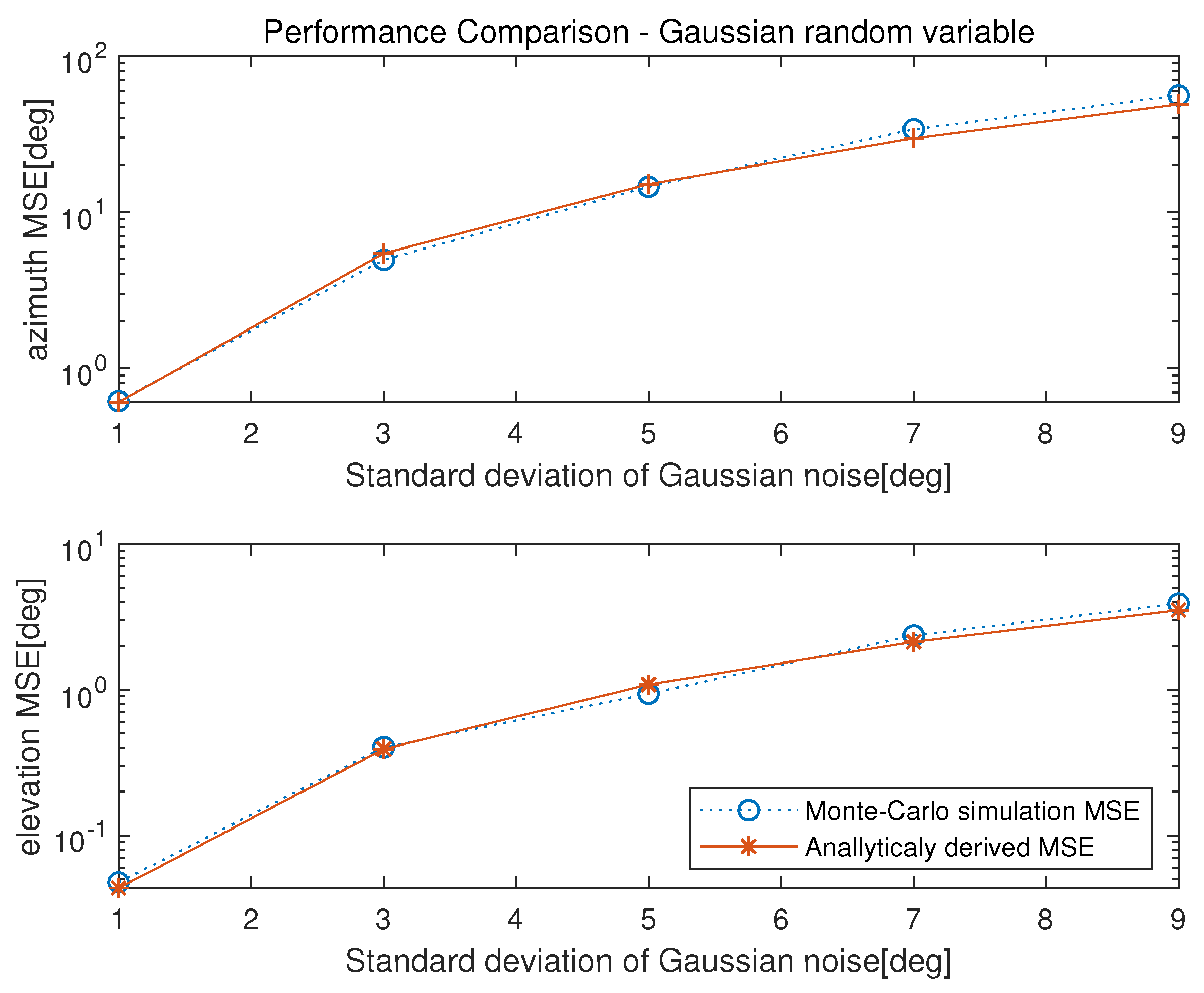
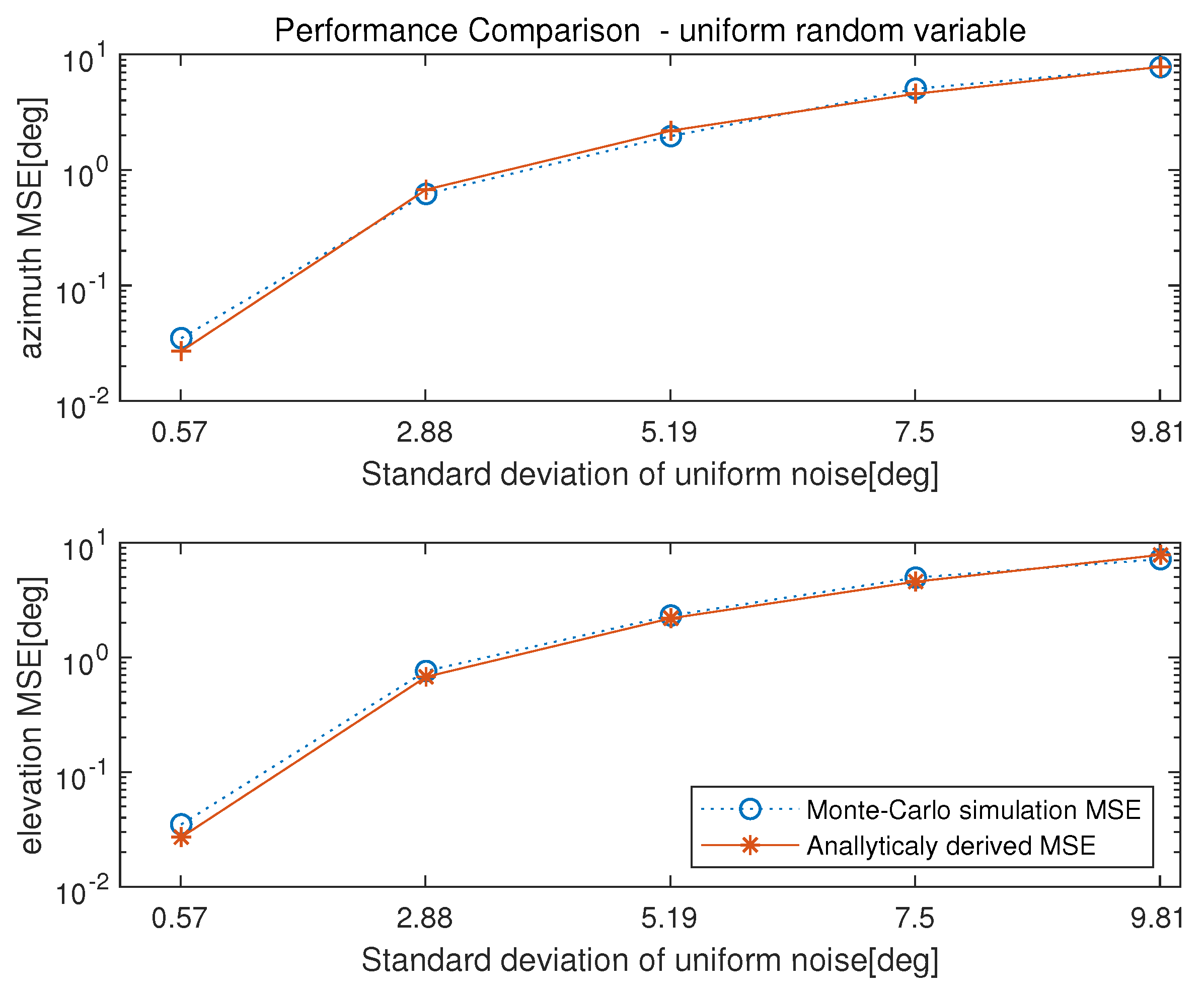
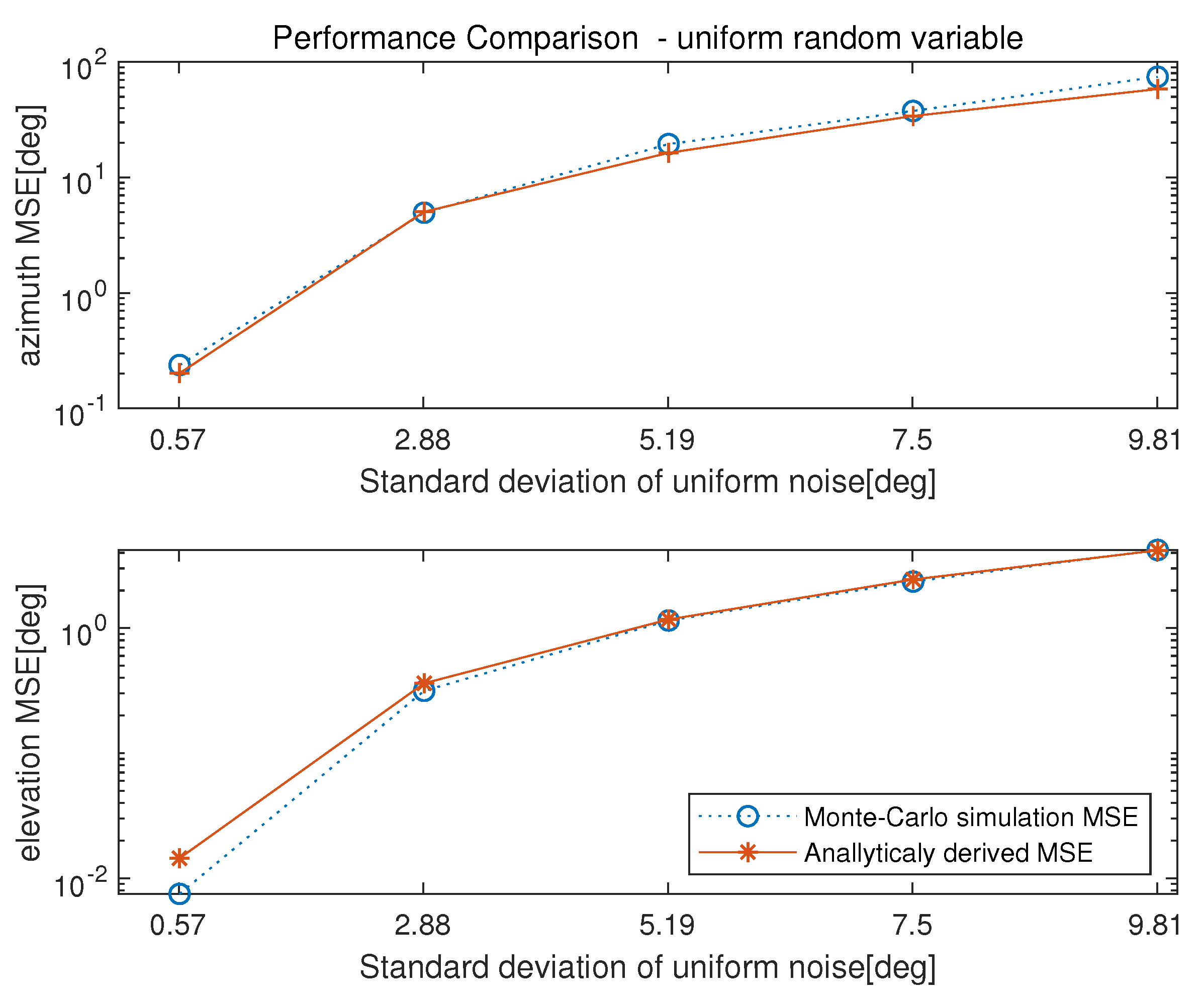
Figure 2, Figure 3 and Figure 4 show the simulation results for the Gaussian random error, and Figure 5, Figure 6 and Figure 7 show the simulation results for the uniform random error. The elevation was set to 15${}^{°}$, 45${}^{°}$, and 75${}^{°}$, and the azimuth was set to 120${}^{°}$ in all cases. It is shown that the MSE of the azimuth is larger than that of the elevation for high true elevation incident signal. On the other hand, it is shown that the MSE of elevation is larger than that of the azimuth for low true elevation incident signal. In all cases, it can be confirmed that the analytic MSEs show agreements with the MSEs of the Monte Carlo simulation.

Figure 2. Performance for Gaussian–distributed phase measurement error with ${\theta }^{\left(0\right)}={120}^{°}$ and ${\psi }^{\left(0\right)}={15}^{°}$. This figure shows the mean square errors (MSEs) of azimuth and elevation with respect to phase error at a signal with low incident elevation. It can be confirmed that the MSE of elevation is larger than that of the azimuth at low elevation (uniform circular array).

Figure 3. Performance for Gaussian–distributed phase measurement error with ${\theta }^{\left(0\right)}={120}^{°}$ and ${\psi }^{\left(0\right)}={45}^{°}$. This figure shows the MSEs of azimuth and elevation with respect to phase error at a signal with medium incident elevation. It can be confirmed that the MSE of elevation is similar to that of the azimuth at medium elevation (uniform circular array).

Figure 4. Performance for Gaussian–distributed phase measurement error with ${\theta }^{\left(0\right)}={120}^{°}$ and ${\psi }^{\left(0\right)}={75}^{°}$. This figure shows the MSEs of azimuth and elevation with respect to phase error at a signal with high incident elevation. It can be confirmed that the MSE of elevation is smaller than that of the azimuth at high elevation (uniform circular array).

Figure 5. Performance for uniformly–distributed phase measurement error with ${\theta }^{\left(0\right)}={120}^{°}$ and ${\psi }^{\left(0\right)}={15}^{°}$. This figure shows the MSEs of azimuth and elevation with respect to phase error at a signal with low incident elevation (uniform circular array). It can be confirmed that the MSE of elevation is larger than that of the azimuth at low elevation (uniform circular array).

Figure 6. Performance for uniformly–distributed phase measurement error with ${\theta }^{\left(0\right)}={120}^{°}$ and ${\psi }^{\left(0\right)}={45}^{°}$. This figure shows the MSEs of azimuth and elevation with respect to phase error at a signal with medium incident elevation. It can be confirmed that the MSE of elevation is similar to that of the azimuth at medium elevation (uniform circular array).

Figure 7. Performance for uniformly–distributed phase measurement error with ${\theta }^{\left(0\right)}={120}^{°}$ and ${\psi }^{\left(0\right)}={75}^{°}$. This figure shows the MSEs of azimuth and elevation with respect to phase error at a signal with high incident elevation. It can be confirmed that the MSE of elevation is smaller than that of the azimuth at high elevation (uniform circular array).

From the upper figures of Figure 2, Figure 3, Figure 4, Figure 5, Figure 6 and Figure 7, it is clear that azimuth MSE increases with the increase of the true elevation angle, ${\psi }^{\left(0\right)}$. On the other hand, from the lower figures of Figure 2, Figure 3, Figure 4, Figure 5, Figure 6 and Figure 7, it is clear that elevation MSE decreases with the increase of the true elevation angle, ${\psi }^{\left(0\right)}$. From Figure 2 and Figure 5, the elevation MSE is greater than the azimuth MSE for small ${\psi }^{\left(0\right)}={15}^{°}$. Note that $\frac{1}{{(sin\left({\psi }^{\left(0\right)}\right))}^2}$ is greater than $\frac{1}{{(cos\left({\psi }^{\left(0\right)}\right))}^2}$ for ${\psi }^{\left(0\right)}<{45}^{°}$.

On the other hand, from Figure 4 and Figure 7, the elevation MSE is smaller than the azimuth MSE for large ${\psi }^{\left(0\right)}={75}^{°}$, which is consistent with (19) and (20) since $\frac{1}{{(sin\left({\psi }^{\left(0\right)}\right))}^2}$ is smaller than $\frac{1}{{(cos\left({\psi }^{\left(0\right)}\right))}^2}$ for ${\psi }^{\left(0\right)}>{45}^{°}$. The observations summarized at the end of Section “Performance analysis of phase comparison interferometer” are validated from Figure 2, Figure 3, Figure 4, Figure 5, Figure 6 and Figure 7.

To see how the azimuth and elevation MSEs are dependent on true azimuth and true elevation of the incident signal for array geometry which is not uniform circular array, rectangular planar array is considered. The array geometry and simulation parameters for rectangular planar array are presented in Table 2. The results for the Gaussian-distributed measurement error are shown in Figure 8, Figure 9 and Figure 10, and those for the uniform-distributed are illustrated in Figure 11, Figure 12 and Figure 13.

Table 2. Simulation condition for arbitrary array.

Parameter	Value
Number of sensors	9
Array architecture	Rectangular Planar Array
Monte-Carlo iteration	1000
Distance of array	0.5$\lambda$

Figure 8. Performance for Gaussian–distributed phase measurement error with ${\theta }^{\left(0\right)}={120}^{°}$ and ${\psi }^{\left(0\right)}={15}^{°}$. This figure shows the MSEs of azimuth and elevation with respect to phase error at a signal with low incident elevation by monte-carlo simulation (rectangular plannar array).

Figure 9. Performance for Gaussian–distributed phase measurement error with ${\theta }^{\left(0\right)}={120}^{°}$ and ${\psi }^{\left(0\right)}={45}^{°}$. This figure shows the MSEs of azimuth and elevation with respect to phase error at a signal with low incident elevation by monte-carlo simulation (rectangular plannar array).

Figure 10. Performance for Gaussian–distributed phase measurement error with ${\theta }^{\left(0\right)}={120}^{°}$ and ${\psi }^{\left(0\right)}={75}^{°}$. This figure shows the MSEs of azimuth and elevation with respect to phase error at a signal with low incident elevation by monte-carlo simulation (rectangular planar array).

Figure 11. Performance for uniformly–distributed phase measurement error with ${\theta }^{\left(0\right)}={120}^{°}$ and ${\psi }^{\left(0\right)}={15}^{°}$. This figure shows the MSEs of azimuth and elevation with respect to phase error at a signal with low incident elevation by monte-carlo simulation (rectangular planar array).

Figure 12. Performance for uniformly–distributed phase measurement error with ${\theta }^{\left(0\right)}={120}^{°}$ and ${\psi }^{\left(0\right)}={45}^{°}$. This figure shows the MSEs of azimuth and elevation with respect to phase error at a signal with low incident elevation by monte-carlo simulation (rectangular planar array).

Figure 13. Performance for uniformly–distributed phase measurement error with ${\theta }^{\left(0\right)}={120}^{°}$ and ${\psi }^{\left(0\right)}={75}^{°}$. This figure shows the MSEs of azimuth and elevation with respect to phase error at a signal with low incident elevation by monte-carlo simulation (rectangular planar array).

In Figure 8 and Figure 11, elevation MSE is greater than azimuth MSE. In Figure 10 and Figure 13, elevation MSE is smaller than azimuth MSE. The dependence of azimuth MSE and elevation MSE on the true elevation is clearly illustrated in Figure 8, Figure 9, Figure 10, Figure 11, Figure 12 and Figure 13. Note that all the observations in Figure 2, Figure 3, Figure 4, Figure 5, Figure 6 and Figure 7 are also true for Figure 8, Figure 9, Figure 10, Figure 11, Figure 12 and Figure 13.

7. Conclusions

In this paper, we have proposed a method of deriving analytic MSEs of azimuth estimates and elevation estimates of signal incident on the uniform circular array. The derived expression is validated from the agreement between the analytically derived expression and the results from the Monte-Carlo simulation in Figure 2, Figure 3, Figure 4, Figure 5, Figure 6, Figure 7, Figure 8, Figure 9, Figure 10, Figure 11, Figure 12 and Figure 13. In the numerical results, it is shown that the azimuth MSE and the elevation MSE are highly dependent on the true elevation of the incident signal rather than true azimuth of the incident signal.

Explicit expressions of the MSEs of the azimuth estimate and the elevation estimate have been derived. The derived expressions are used to determine how accurate the interferometer algorithm under measurement uncertainty is. It has been illustrated in the numerical results.

Another contribution of the proposed scheme is that the azimuth estimation error in (15) and the elevation estimation error in (16) can be obtained without exhaustive search of interferometer cost function in (2). In Monte-Carlo simulation, two-dimensional search with respect to $\theta$ and $\psi$ of the cost function in (3) should be performed, which is two-dimensional nonlinear optimization. On the other hand, the expressions in (15) and (16) are closed-form expressions of the azimuth error and the elevation error. Therefore, computationally intensive numerical optimization can be removed. In addition, the MSEs of the azimuth estimate and the elevation estimate as well as the estimation errors of the azimuth estimate and the elevation estimate are available in (18) and (19).

In addition, in numerical optimization of (3), the estimates are highly dependent on the search range and search step, which implies that the estimates from numerical optimization may be inaccurate if search step and search range are not properly chosen.

In summary, the estimate from the numerical optimization of (3) has two demerits of computational cost and dependence on search step and search range. In the proposed algorithm, since the azimuth estimate and the elevation estimate are obtained from (15) and (16), and the MSEs are obtained from (18) and (19), two demerits of the Monte-Carlo simulation-based performance analysis can be removed.

We assume that an additive noise on the antenna elements is Gaussian distributed or uniformly distributed. Noise at each antenna is spatially white.

In the case of azimuth/elevation estimation of an incident signal using the UCA, it has been shown that the azimuth estimate and the elevation estimate associated with the interferometer algorithm can be expressed in the closed-form as (15) and (16), respectively.

The closed-form expressions of the MSEs of the azimuth estimate and the elevation estimate can be obtained from (18) and (19), respectively, without computationally intensive Monte-Carlo simulation.

The dependence of the azimuth MSE and the elevation MSE on the true elevation has been derived. The derived expressions in (18) and (19) are validated from the agreement between the simulation-based MSEs and the analytically-derived MSEs.. The results is illustrated in Figure 2, Figure 3, Figure 4, Figure 5, Figure 6, Figure 7, Figure 8, Figure 9, Figure 10, Figure 11, Figure 12 and Figure 13.

From (18) and (19), it can be confirmed that the azimuth estimation error is the dominant error for the small true elevation angle, and that the elevation estimation error is dominant for the large true elevation angle. More specifically, the small true elevation angle and the large true elevation angle correspond to ${\psi }^{\left(0\right)}<{45}^{°}$ and ${\psi }^{\left(0\right)}>{45}^{°}$, respectively.