Relational Positioning Method for 2D and 3D Ad Hoc Sensor Networks in Industry 4.0

Featured Application

Position location information plays a crucial role in the automated and adaptable operation of Industry 4.0, allowing sensor fault detection as well as operators localization. The development of 3D positioning techniques is crucial for massive sensor network operability imposed by the Internet of Things. Several network protocols depend on position location information for security and routing purposes. Alternative positioning techniques are necessary for new paradigms imposed by new network applications. The proliferation of 3D applications in Industry 4.0 demands alternative 3D location algorithms.

Abstract

Industry 4.0, or smart factory, refers to the fourth industrial revolution, as a result of which it is expected that massive sensor deployment, high device connectivity, automation, and real-time data acquisition support improve industrial processes. Sensor fault detection and operator tracking allow adequate performance of the sensor network supporting Industry 4.0, and sensor localization has become crucial to enable sensor fault detection. Hence, the development of new localization methods is necessary for environments where GPS localization technology is unfeasible. Furthermore, position location information (PLI) is a crucial requirement for the deployment of multiple services and applications in wireless ad hoc and sensor networks supporting Industry 4.0. Three-dimensional (3D) scenarios are considered to extend the applicability of PLI-based services. However, PLI acquisition presents several challenges within any 3D ad hoc sensor network paradigm. For instance, conventional triangulation algorithms are often no longer applicable due to the lack of direct land-fixed references and the inclusion of a third-dimension coordinate. In this paper, a PL relational searching algorithm suitable for 2D and 3D ad hoc environments was formulated in terms of a discretized searching space and a vertex weight assignment process according to distance relationships from anchor nodes to the node to be located on a feasibility space. The applicability of the proposed algorithm was examined through analytic formulation and simulation processes. Results show small distance errors (less than 1 m) are achievable for some scenarios.

1. Introduction

On a daily basis, position location (PL) becomes a more important issue in wireless systems for security and law enforcement purposes, as well as for resource management, new location-based services (LBSs), and applications (LBAs). Thus far, most of the literature has been focused on planar scenarios. However, sensor networks and the Internet of Things (IoT) have become pervasive concepts that are expected to be used in billions of devices with multiple applications. As an example, the number of IoT-connected devices in 2018 was about 7 billion. Nevertheless, the value of IoT and sensor networks is often related to location information. Therefore, the importance of 3D localization becomes more relevant, as it enables a wide variety of new LBS and new LBA.

The concept of Industry 4.0 denotes the emergence of smart factories where automated and decentralized production is enabled by the Internet of Things (IoT). In Industry 4.0, all objects in the factory (i.e., sensors, tools, actuators, etc.) are meant to be connected and communicating with each other, in order to make possible automated and smart adaptive production. In smart factories, it is possible to dynamically adapt the factory operation depending on the operator’s location. This implies the knowledge of the position of all the involved operators. Additionally, position location information is crucial for sensor fault detection, which ensures an adaptive factory operation. This creates the necessity for developing alternative position location methods for environments in which GPS systems or traditional indoor localization systems are not able to provide information, [1].

In modern network scenarios, position location is necessary to assist network tasks such as routing, resource management, and the delivery of location-aware services. However, in ad hoc and sensor networks, connectivity constantly changes due to variations in propagation conditions, and node activity or node motion, and these variations create changes in the network topology, [2,3]. In addition to global navigation satellite systems (GNSSs) that provide 3D geolocation for outdoor applications, most existing positioning techniques deal with planar location environments that are not sufficient for many applications, [4]. Although GNSS has been in place for many years with different technologies, currently, its availability and accuracy are often insufficient for indoor applications. It is recognized that 3D localization is necessary for several applications, such as in emergency call services in tall building environments, museum guides, warehouse stock management, crew monitoring, drone localization, sensor deployment, etc. [5]. Additionally, emerging applications, such as event monitoring for vehicular networks (VANET) [6] or special situations for the safety and security of people in smart cities, can be assessed by sensor networks, when accurate sensor location information is available.

In the IoT context, location information enables the implementation of new protocols in several functions of the network layer such as routing, sensor energy harvesting, and security. Similarly, it is responsible for enabling multiple applications such as asset tracking, connected vehicles, smart appliances, tracking of people by wearable devices, assisted living, etc. Therefore, innovative localization methods need to be developed in order to adapt to the new paradigms imposed by the massification of heterogeneous sensor nodes.

In this paper, we introduce a new relational searching localization method that is not based on any previous localization technique. Some of its advantages are that distances are estimated based on a hop count criterion, and a very low number of known location nodes or anchors are needed to provide sensor location estimation. These characteristics make it suitable for IoT environments, where low-equipped sensors with very low transmission ranges need to be considered. We present a location-searching method on a discretized space defined by available anchor nodes (ANs). The method used sole distance relationships between ANs and the node of interest, rather than mean square optimization, to develop likelihood indicators for vertices in the searching space according to those distance relationships. Since the process occurred in location systems, observations were prone to impairments due to errors in distance estimation. In addition, the absence of direct connectivity from nodes to ANs is observed in ad hoc routes that depart from a line-of-sight trajectory. The proposed methodology is adequate for 2D and 3D localization, and its performance was assessed throughout simulations assuming different node densities, transmission ranges, and the number of available ANs. Results under different scenarios show a remarkable performance of the method reaching a small distance error (less than 1 m) for some scenarios. Simulation results show that, compared with the 3D positioning algorithm introduced in [7], the proposed method achieves a significant improvement (approximately 50% improvement when combined with finer discretization).

The rest of the paper is as follows: In Section 2, a discussion on related research about localization in 2D and 3D situations is provided. In Section 3, we introduce the relational location-searching method proposed in the paper, starting with a 2D setup and extending it to the 3D scenario. In Section 4, results are presented with their corresponding discussion. Lastly, Section 5 provides the conclusions.

2. Related Research

Traditional localization methods using trilateration are commonly used in 2D for the line of sight (LOS) wireless scenarios, resulting in a good performance in the presence of small distance estimation errors [8]. However, those methods do not deal with the 3D multi-hop wireless sensor scenario, in which one generally finds environments with no LOS between nodes and anchors or access points (AP). Thus, range estimations from anchor nodes (with known coordinates) to the node to be located can be based on the aggregation of hop lengths in the connecting paths, which leads to an additive distance error, [9], impairing the node-to-anchor distance estimation process.

In ref. [10], the authors propose a beacon-based geometric localization method for 2D sensor networks, where a node initially chooses two reference points, then they create what they call the node’s residence area by the range intersection of the two reference points. Subsequently, the node differentiates its estimated position within the residence area using a third reference point, by approximating the radius and half-length of the chord with respect to one of the reference points. Then, the radius and half-length of the chord are used to estimate the sagitta of an arc. Finally, the node estimates its position using the radius, half-length of the chord, and sagitta of an arc. There are several reported works for 3D localization, some of them proposed for indoor environments, where the position of a node is estimated by relating the actual observation with a set of collected observation data previously taken by a set of sensors deployed strategically in the indoor scenario. In ref. [11], the authors provide a survey of indoor position location systems updating the new transmission technologies.

In ref. [12], the authors present a survey for indoor localization techniques in the context of IoT. In this paper, the authors discuss different indoor localization systems focusing on user device tracking. They develop an evaluation framework to compare existing indoor localization techniques focusing on the IoT demands. They divide the existing indoor localization techniques into two classifications: monitor-based localization (MBL) and device-based localization, (DBL). In the MBL, a set of anchor nodes passively obtains the position of the user or entity connected to the reference node. In the DBL, the user device uses some reference nodes (RNs) to obtain its relative location. Their evaluation framework focuses on several IoT relevant parameters such as cost, service availability, energy efficiency, accuracy, scalability, etc.

Outdoor 3D localization has been commonly conducted through GNSS systems, [4]; however, there is a need to develop alternative 3D PL techniques suitable for places where satellite coverage is not available or limited. In [13], the authors present a localization system for 3D ad hoc networks using aerial sensor nodes equipped with UWB devices to provide 3D positioning capabilities. The proposed technique in [13] firstly uses a local coordinate system that is defined using sensor nodes. Secondly, a calculation of the sensor’s coordinates is performed based on a regular trilateration technique. Finally, the sensor nodes progressively become anchor nodes as their locations are estimated. The method is evaluated in a single hop scenario. The method relies on nodes upgrading with UWB devices and antennas to provide 3D positioning capability. The system performance depends on the goodness of distance estimation. In [14], the authors propose a received signal strength indicator (RSSI) range-based 3D localization method for wireless sensor networks, where they formulate a degree of co-planarity and combine it with the traditional DV-Distance algorithm. Then, the set of four anchor nodes with the best degree of co-planarity (the flattest) is selected to calculate the node-of-interest location using simple quadrilateration. After a node calculates its position, it is promoted as anchor node assistant to improve the positioning coverage. Finally, a quasi-Newton method is used to optimize the positioning result.

In ref. [15], the authors propose a sequence localization algorithm based on the use of a 3D Voronoi diagram. The Voronoi diagram is used to divide the working space depending on the real beacon nodes (known location nodes) and construct a rank sequence table of virtual beacon nodes (determined after partition). This algorithm uses RSSI estimations between nodes as a reference to correct the measured distances and to fix the location sequence of unknown nodes. Then, the algorithm commands a weighted location estimate with N valid virtual beacon nodes by a normalization process of rank correlation coefficients.

In a different approach, the authors of [7] propose a method that is based on the convenient deployment of access points (APs) with known coordinates and on the Manhattanization of the network space. A set of algebraic relationships is defined for the node’s coordinates based on distances from APs to the node of interest. In addition, a maximum a posteriori probability (MAP) criterion is used to improve estimated distances and to improve the performance of the algebraic method. This method is evaluated in multi-hop scenarios, and the distance between nodes is estimated based on the hop count criterion [16]. The main contribution is a new method for location estimation suitable for 3D network spaces. Table 1 summarizes some characteristics of the 3D localization methods explained above, as well as some evaluation performance and scenarios setup.

Table 1. Summary of outdoor 3D PL methods.

3D PL Method	Principle	Accuracy
A 3D ad hoc localization system using aerial sensor nodes [13].	Traditional triangulation using UWB equipped aerial nodes.	In terms of standard deviation σ. They achieve 0.24 m σ.
An improved 3D localization algorithm for the wireless sensor network [14].	Traditional quadrilateration combined with an optimization method.	Localization error is normalized to r0. Achieving error of 0.35 r0 for 17 ANs.
3D localization algorithm based on Voronoi diagram and rank sequence in wireless sensor network [15].	Sequence localization using a Voronoi table to divide space. Then, construct a rank sequence for virtual beacon nodes.	Localization error is normalized to r0. Achieving 0.12 r0 for 8 ANs.
3D position location in ad hoc networks: a Manhattanized space [7].	Algebraic Manhattan restrictions.	In terms of mean Euclidean distance error, normalized to the Tx range r0. They achieve 0.8 r0 for 4 anchors.

In ref. [17], the authors present a survey of multidimensional scaling (MDS) based localization techniques. These are range-free localization techniques that use proximity information instead of actual distance measurements. MDS keeps the important information while reduces multidimensional data into a lower-dimensional space. In this paper, the authors present an overview of the different variants of outdoor and indoor MDS-based localization systems. They also present some 3D MDS-based localization methods for WSN and discuss how some proposed methods for 2D are not effective in 3D environments, as complexity increases due to several factors, such as node deployment, increment of anchors needed for location calculation, connectivity, and physical obstructions.

As explained before, in this paper, we present a different positioning approach based on distance relationships and on a likelihood function. The relational positioning method formulates a searching equation based on a likelihood function that depends on a weights proportion where the points closest to the node to be located will have greater weight according to an assignment based on the ratio of distance relationships between ANs and the node of interest.

For the sake of simplicity, we describe the method both for planar and 3D scenarios in the following sections. Note that in this paper, we present the conceptualization of a new 3D localization method and its evaluation in different network scenarios. However, concerns about the implementation of the method in terms of the network layer perspective (e.g., control messages, message passing, etc.) are not necessary to assess the performance of the proposed algorithm.

3. Relational Positioning Method

In the current positioning system, we propose to determine the location of a node n₀ in a given area that is assumed to be a subset of a region R, defined by the convex hull contained by a number of ANs. Although our main concern is with 3D localization, for explanatory purposes, we initially consider a planar 2D scenario in which we discretize the region according to an immaterial regular square lattice with a basic separation unit L. We also assume that the locations of ANs and the node to be located coincide with some vertices v in the lattice. In the absence of further information, the uncertainty of the location of the node equates to log(N_c), where N_c denotes the number of cross points in the lattice, and the node of interest is considered to be equally likely to be located at any of those cross points of the lattice. The proposed method allows us to reduce the location uncertainty through likelihood proximity estimates.

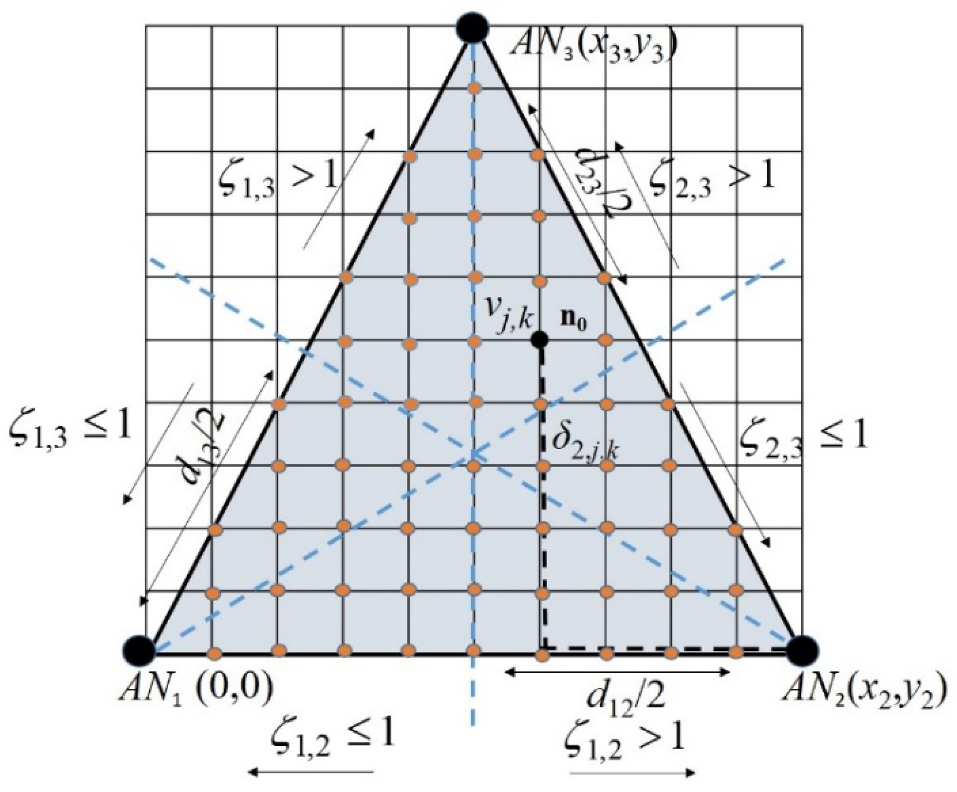
3.1. Two-Dimensional (2D) Localization

For explanatory purposes, we first consider a planar scenario, and later the method is extended to a 3D scenario. A vertex in the lattice at cross point (j,k), with coordinates ($x_{v_{j,k}}, y_{v_{j,k}}$), is denoted as v_j,k and it is meant to be δ_i,(j,k) Manhattan units apart from AN_i with coordinates (x_i, y_i). The Manhattan distance between AN_i and vertex v_j,k is defined as ${\delta }_{i,\left(j,k\right)}=\frac{| x_i-x_{v_{j,k}}|+|y_i-y_{v_{j,k}}| }{L}$, where L is the Manhattan unit. Thus, the node of interest n₀ is assumed to be at the unknown vertex v_j,k in the discretized region, and it will have an associated set {δ_i,(j,k)}, i = 1, 2, 3, of Manhattan distances [18] to the corresponding AN_i, (see Figure 1). This assumption is not necessarily true in real environments; however, the searching method perceives this as distance estimation noise and makes a search of the most likely vertex v_j,k for location estimation of node n₀. This process is explained in detail in this section, and it is further developed when the 3D localization method is explained.

Figure 1. A 2D scenario for three ANs in a triangle.

Actual Manhattan distances from ANs to n₀ at vertex v_j,k, may not be available. Although in an ad hoc network, they can be estimated by multiplying the mean length of a hop and the hop count in the shortest path linking the concerned node and the AN [16]. Estimated distances from AN_i to n₀, Δ_i,(j,k), may depart from the corresponding Manhattan distances δ_{i, (j,k)}; this is Δ_i,(j,k) = δ_i,(j,k) + e_i, (j,k), where the term e_i,(j,k) accounts for an error associated with the estimation method, and it is often related to the node density and routing algorithm [16]. Note that the actual Manhattan distance between any pair of anchors AN_i (i = 1,2,3) is determined from the known AN_i (i = 1, 2, 3) coordinates, as stated above.

In order to construct a location likelihood matrix ρ = [$\rho$_j,k], we define an initial matrix W = [w_jk], where we assign an initial weight w_j,k = 1 to each vertex v_j,k lying inside the convex hull containing the AN_i, and otherwise, w_j,k = 0, meaning that each vertex can equally be a candidate for the node n₀ location. Weights w_j,k will iteratively be changed, allowing to correspondingly define a location likelihood matrix ρ = [$\rho$_j,k], where$\rho$_j,k$=\frac{w_{j,k}}{{\sum }_{j,k}{w}_{j,k}}$ is the probability (likelihood) of the node being at vertex v_j,k. Note that${\sum }_{j,k}{\rho }_{j,k}=1$.

The weights $w_{j,k}$ can further be modified, bearing in mind the relative distances to different AN nodes. For instance, let Δ_i,(j,k) and Δ_m,(j,k) be estimated distances from n₀ to AN_i and AN_m, respectively. As many interference elements such as physical barriers, multipath phenomena, moving objects and measurement errors may impair distance estimates, our approach is based on the hop count criterion; that is, Δ_i,_(j,k) is proportionally approximated to the number of hops in the route connecting AN_i to node n₀ assumed to be at vertex v_j,k. Although we introduce some quantizing errors, making distance estimation dependent upon the hop count criterion leads to the proposed method becoming more robust to propagation impairments than the previously mentioned methods.

We define an ANs pair (i,m) proximity ratio as ζ_i,m = Δ_i,(j,k)/Δ_m,(j,k), i, m = 1, 2, 3, i ≠ m. Then, for those vertices in the region of interest (that is, for w_i,k ≠ 0), their weights w_i,k are incremented according to w_i,k = w_i,k + 1, for those locations (j, k) where ζ_i,m ≤ 1. In this form, the weights are heavier for those nodes in closer proximity to AN_i, and likelihood indexes $\rho$_j,k are accordingly modified, denoting the more likely location for n₀. With these likelihoods ${\rho }_{j,k}$, we can use entropy to measure the uncertainty of a vertex, and thus, we can focus on those vertices with less uncertainty. Entropy for the area/space discretized according to L can be expressed in this case as follows:

$$H_L\left(v_{j,k}\right)=-{{\displaystyle \sum }}_{j,k}{\rho }_{j,k}\log \left({\rho }_{j,k}\right)$$

(1)

Note that the likelihood$\rho$_j,k assignment process is conducted a number of times given by the combinations _NC₂ for all the pairs of ANs (where N is the number of available ANs). As explained before, the proposed position location method diminishes the uncertainty or entropy by modifying the location likelihood of the nodes in the feasibility space using distance relationships.

In Figure 2a, vertices increment their weights according to ζ_1,2 ≤ 1, in Figure 2b according to ζ_1,3 ≤ 1, and in Figure 2c according to ζ_3,2 < 1, which is the same as ζ_2,3 > 1, i.e., vertices closer to AN₃ increase their weights.

Figure 2. Weight assignment distribution for tree ANs and for relations (a) ζ_1,2 ≤ 1, (b) ζ_1,3 ≤ 1, and (c) ζ_2,3 > 1.

Up to this stage, we worked with three ANs in order to keep the infrastructure requirements as low as possible. However, note that the feasibility vertex set can be reduced if more ANs are available. In Figure 3, we increase the number of ANs in the scenario illustrated in Figure 2, and it is possible to see that by applying an additional relation as ζ_1,4 ≤ 1, the feasible vertex set is reduced.

Figure 3. Illustration of a feasible vertex set reduction when four ANs are available and ζ_1,4 ≤ 1 is applied.

Recall that$\rho$_j,k, is the probability (likelihood) of vertex v_j,k, to be the position of n₀, where vertex probabilities ρ_j,k, change after every relationship index ζ_i,m is considered for weight assignment; this implies that the entropy function H_L(v) also changes after every stage. In Figure 4, we can see how entropy behaves after every ζ_i,m is applied for the representative example explained in Figure 2 and Figure 3.

Figure 4. Location entropy for three ANs scenarios using different relational stages.

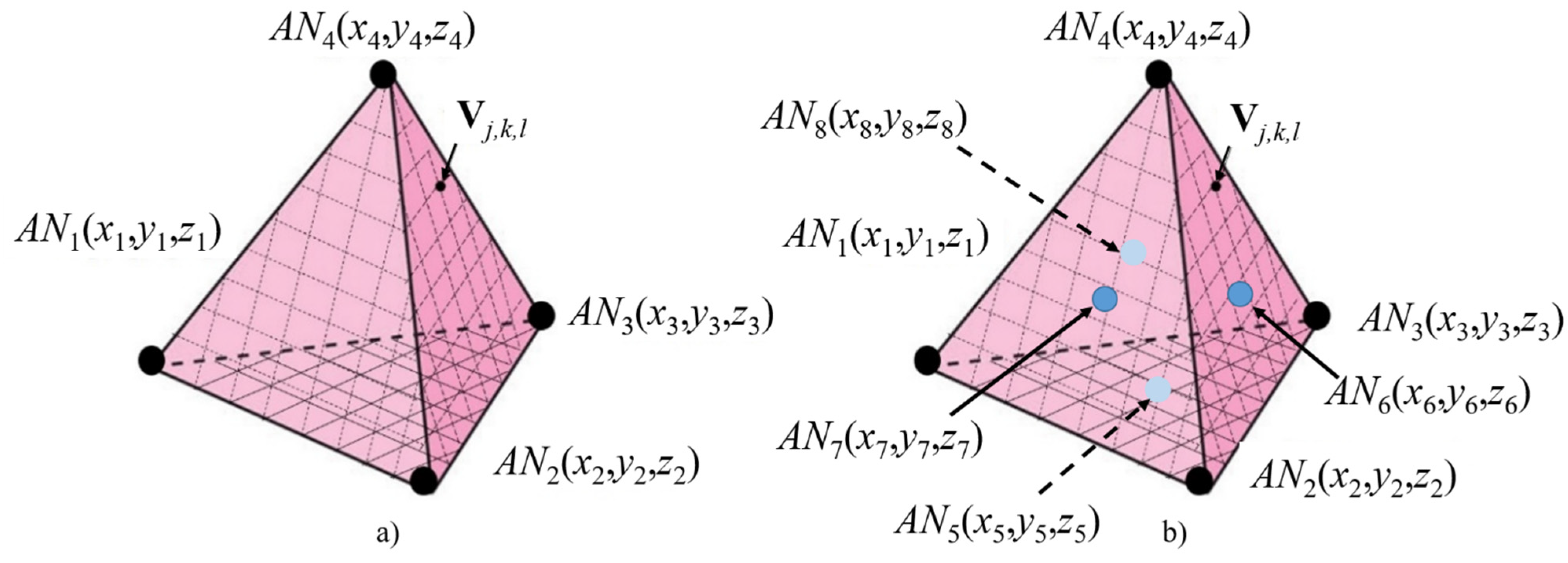
3.2. Three-Dimensional (3D) Localization

In the case of 3D scenarios, the node to be located is meant to be within the 3D convex hull volume V defined by the ANs. For instance, in the case of four equidistant Ans, the convex hull coincides with a regular tetrahedron, as is illustrated in Figure 5a.

Figure 5. The 3D Scenario for (a) four available ANs and (b) up to eight available ANs.

As explained before, a discretization of the searching space is conducted with vertices v_j,k,l in a three-dimensional regular grid with step L. The weight w_j,k,l assignment process is extended to 3D, where (i,k,l) stands for the coordinates in the searching space, though it remains based on distance relationships ζ_i,m. As an example, consider the case in which n₀ is contained within a regular tetrahedron with ₄C₂ = 6 (where ₄C₂ is the combinatorial coefficient) relative distance comparisons.

It is anticipated that performance improvements can be achieved when the number of ANs is increased in the same volume or area as more distance relationships, e.g., ₅C₂, from ANs to n₀ can be used. Therefore, we obtain a different weight assignment from that obtained for four ANs in the tetrahedron. As stated before, a discretization process is performed first. Secondly, the weight assignment process is carried out according to distance relationships ζ_i,m. Finally, the searching equation as that shown in (2) can be reformulated based on the distance sets Δ_{i, (j,k,l)}, and δ_i,(j,k,l), where sub-indices 1 ≤ i ≤ m refer to the corresponding AN_i, and (j,k,l) refers to the coordinate (x, y, z) in a tridimensional space.

As stated before, uncertainty reduction helps to decrease the searching space, allowing lower processing time, required processing capacity, and power consumption. The final location will be determined by an optimal searching process over the feasible region R* = {v_j,k,l, w_j,k,l≠0} where a minimum-error searching equation is formulated as follows:

$${\min }_{j,k,l}[{\rho }_{j,k,l}^{-1}\sum _i|{\Delta }_{i,\left(j,k,l\right)}-{\delta }_{i,\left(j,k,l\right)}|],$$

(2)

where ${\rho }_{j,k,l}=w_{j,k,l}/{\displaystyle \sum _{j,k,l}{w}_{j,k,l}}$ and 1 ≥ i ≥ 4.

A vertex v_j,k,l will be the solution to the localization problem, if such vertex gives the minimum difference between its associated distance set δ_i,(j,k,l) and the estimated distances from ANs to node n₀, Δ_i,(j,k,l), multiplied by the inverse of ${\rho }_{j,k,l}=w_{j,k,l}/{\displaystyle \sum _{j,k,l}{w}_{j,k,l}}$.

Note that the region of interest R can have different shapes and sizes depending on the available ANs and their locations. Additionally, it is worth noting that the inclusion of additional ANs can improve localization accuracy. In the following section, we deduce that uncertainty is reduced significantly when the proposed searching method is combined with a finer discretization which helps to achieve significant improvements. We also evaluate how the weight assignment process can reduce uncertainty. Additionally, the performance of the proposed method is assessed under different scenarios.

We summarize the 3D relational positioning method with the following set of steps:

• Discretize the working operational area or space, obtaining v_j,k,l;
• Calculate the Manhattan distance from AN_i to v_j,k,l, ${\delta }_{i,\left(j,k,l\right)}$;
• Obtain the route from ANs to the node of interest n₀;
• Calculate distance from AN_i to n₀ based on the number of hops in the route Δ_i,(j,k,l);
• Calculate distance relationships between every pair of ANs as ζ_i,m = Δ_i,(j,k,l)/Δ_m,(j,k,l);
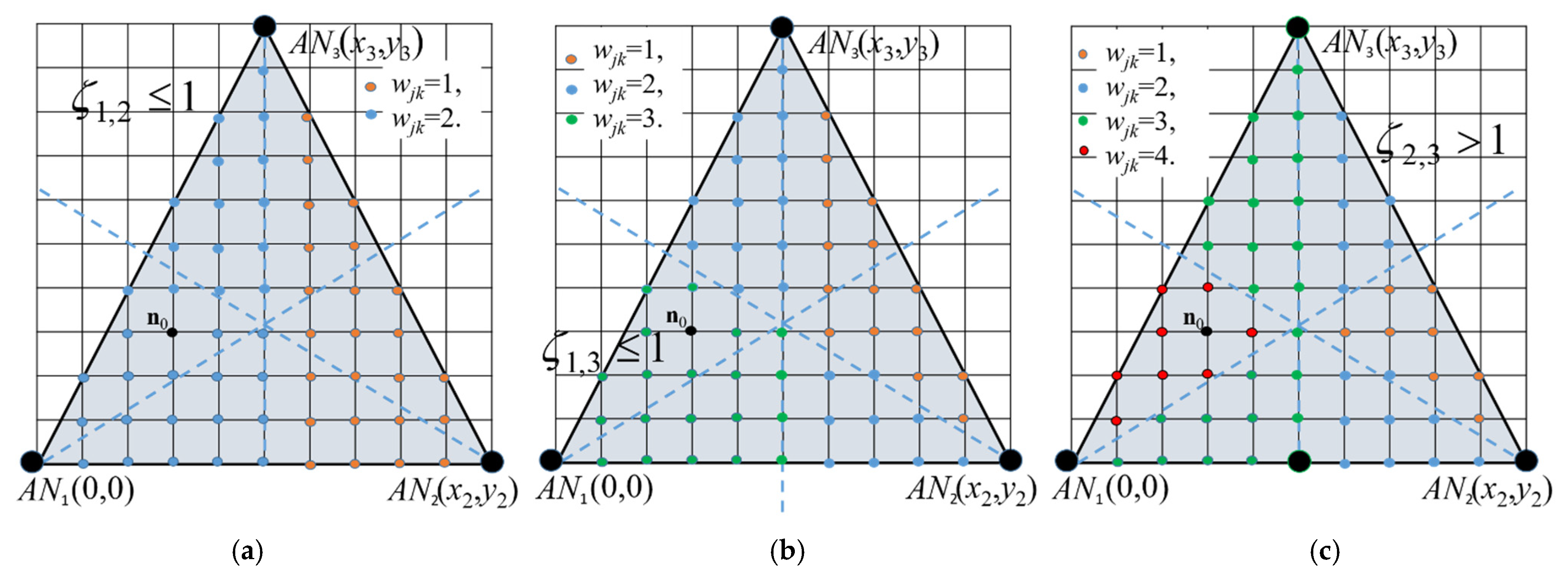
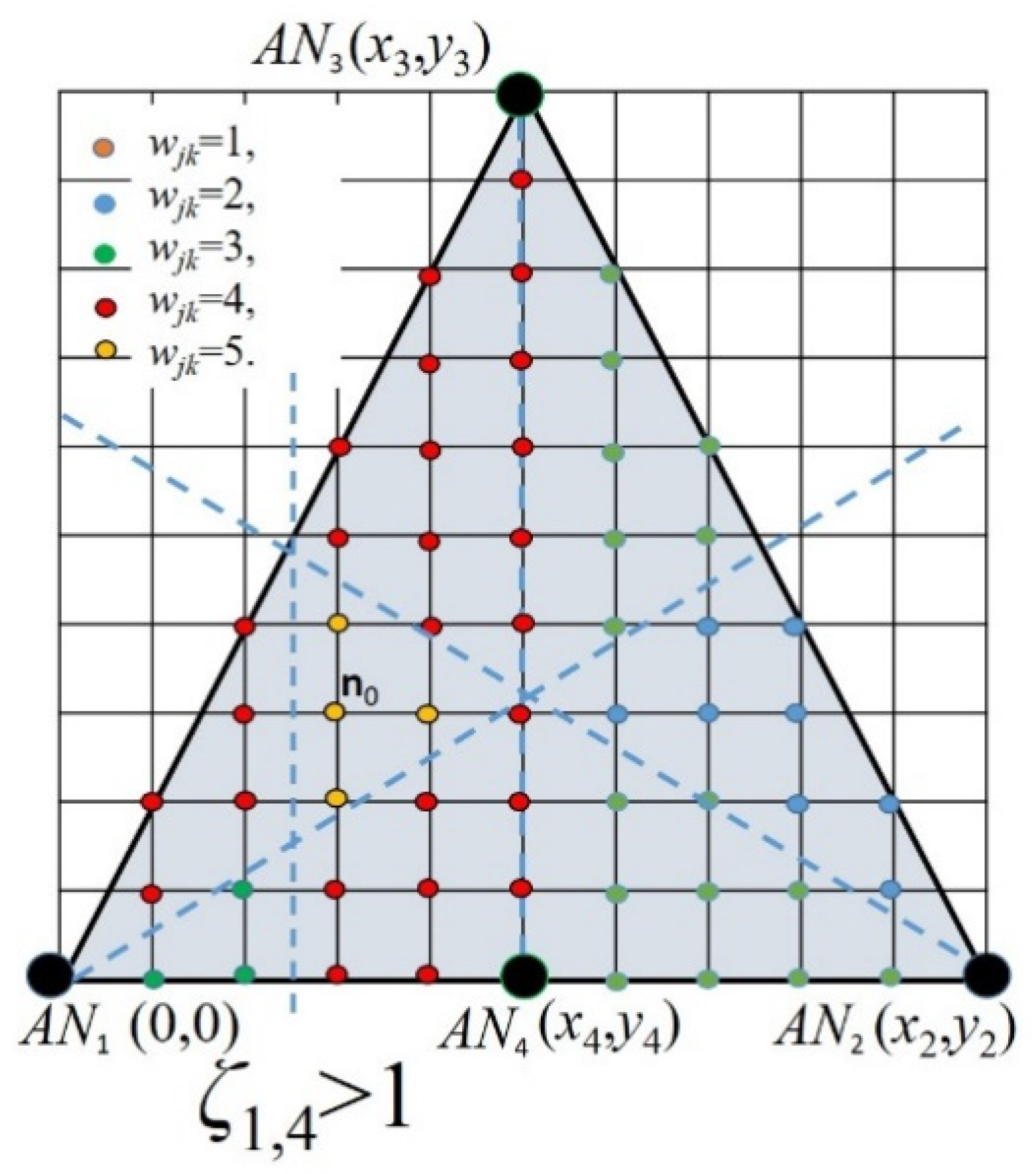
• Modify vertex weight w_j,k,l for every pair of ANs, as follows: If ζ_i,m < 1, then the node is closer to AN_i than to AN_m, hence every vertex weight w_j,k,l closer to AN_i is increased by 1. Otherwise, increase by 1 every vertex weight w_j,k,l closer to AN_m;
• Calculate the location likelihood matrix $\rho$_j,k,l$=\frac{w_{j,k,l}}{{\sum }_{j,k,l}{w}_{j,k,l}}$;
• Perform the minimum-error searching based on equation ${\min }_{j,k,l}[{\rho }_{j,k,l}^{-1}\sum _i|{\Delta }_{i,\left(j,k,l\right)}-{\delta }_{i,\left(j,k,l\right)}|]$ to find the estimated location.

4. Simulations and Results

In this section, we evaluate the performance of the proposed method based on the average quadratic error criterion. Note that influences from protocols of the network layer or other layers are not considered in the evaluation, because results may be affected and such protocols change for different technologies, and therefore, we would have no clear trends of the performance of the method. First, we evaluate the PL relational searching method under two-dimensional network scenarios with three and four ANs.

4.1. The 2D Evaluation

To evaluate the performance of the proposed PL searching method, and without loss of generality, we set ANs’ locations in an equilateral triangle defined by ANs coordinates as follows: AN₁(0,0), AN₂(d,0), AN₃(d cos$\frac{\pi }{3}$, d sin$\frac{\pi }{3}$), when three ANs are available (as in Figure 1), and as in a regular square AN₁(0,0), AN₂(d,0), AN₃(d,d), AN₄(0,d), when four ANs are available. Nodes are deployed randomly according to a uniform pdf in the working area or space; that is, nodes’ coordinates are selected as x~U(0,d) and y~U(0,d). The node to be located is also randomly selected.

In the following analysis, we evaluate the average quadratic error of the Euclidean distance between the estimated position and the true position ε, and we normalize it to the AN separation distance d, which is related to ANs’ coordinates and defines the size of the network scenario, i.e., ε/d. Error normalization is conducted in order to relate results under different scenarios (2D and 3D) in terms of the same scenario constructive variable d (associated with ANs coordinates). This is carried out in order to keep a fair comparison of performance between different scenarios.

In the following simulations, we analyze the positioning method under different network conditions. For the 2D scenarios, we perform a basic analysis considering different values of the coverage radius r₀ and number of nodes n_, in order to prove the feasibility of the method for 2D networks, and we also show that location estimation is improved when the number of ANs is increased.

For instance, in Figure 6, we can observe the performance of the relational searching method for two different 2D scenarios with the same working area, where three and four ANs are considered. In this figure, we can see that a consistent improvement from about 7% to 18% is achieved when we increment the number of ANs from three to four. Additionally, we can see a slight improvement on the algorithm performance as we increase the number of nodes from n = 30 to n = 40, which can be explained by an expected improvement on routes obtained from ANs to the node to locate. As the hop count method is used to estimate distances, better routes may imply better distance estimations. Note that there is an increment of the normalized positioning error ε/d when the maximal transmission range r₀ is increased from r₀ = 2.5 m to r₀ = 5 m. This can also be explained because worse distance estimations from ANs to the node to be located are obtained (as the hop count distance estimation is selected) when r₀ is increased. The performance obtained for r₀ = 2 m, which is worse than the performance for r₀ = 2.5 m can be explained due to the low node density.

Figure 6. Error analysis for different transmission ranges, r₀, using three and four ANs in a 2D scenario with d = 10 m, n = 30, and n = 40 nodes.

In order to consider more realistic scenarios than those evaluated in Figure 6, the AN₃ coordinates are modified. Note that when changing x₃, irregular triangle scenarios are generated. In Table 2 we can observe these results in terms of the normalized localization error ε/d, for different maximal transmission range r_0, n = 40, and different x₃ values. In Table 2, we can infer that the location estimation given by ε/d stays stable as the analyzed shape scenario is changed. Even more, we can find some cases in which the normalized error decreases, as better relationships might be found.

Table 2. Error (ε/d) analysis for different triangle shapes (“x” coordinate of AN₃).

r0(m)	2	2.5	3.333	5
x3 = d sin$\frac{\pi }{3}$	0.1606	0.1410	0.1553	0.209
x3 = d sin$\frac{\pi }{3}$ ± 1	0.1380	0.1308	0.1520	0.2025
x3 = d sin$\frac{\pi }{3}$ ± 2	0.1415	0.1328	0.1448	0.2034
x3 = d sin$\frac{\pi }{3}$ ± 3	0.1406	0.1106	0.1301	0.1810
x3 = d sin$\frac{\pi }{3}$ ± 4	0.1396	0.1220	0.1518	0.1860
x3 = d sin$\frac{\pi }{3}$ ± 5	0.1390	0.1163	0.1545	0.2005

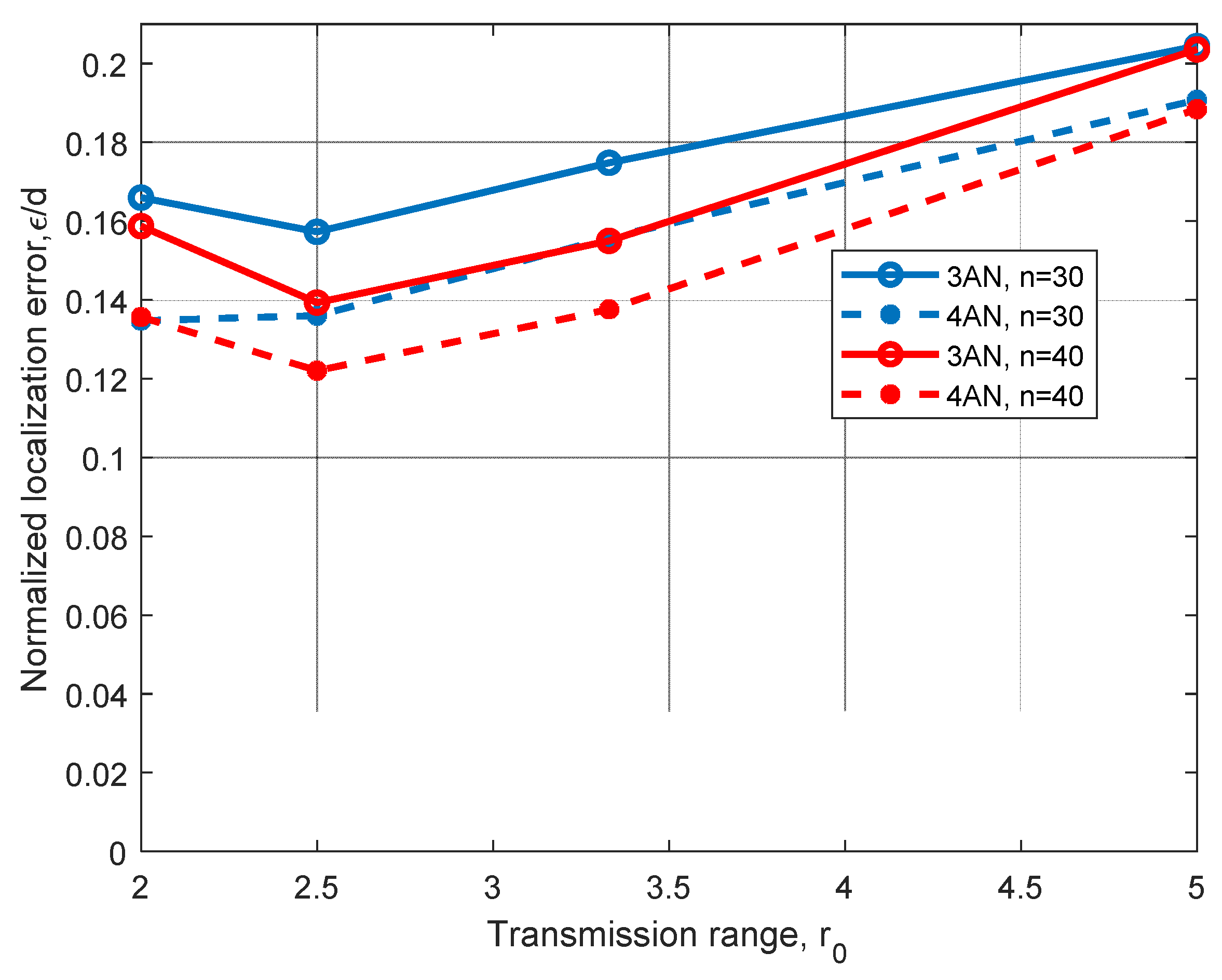
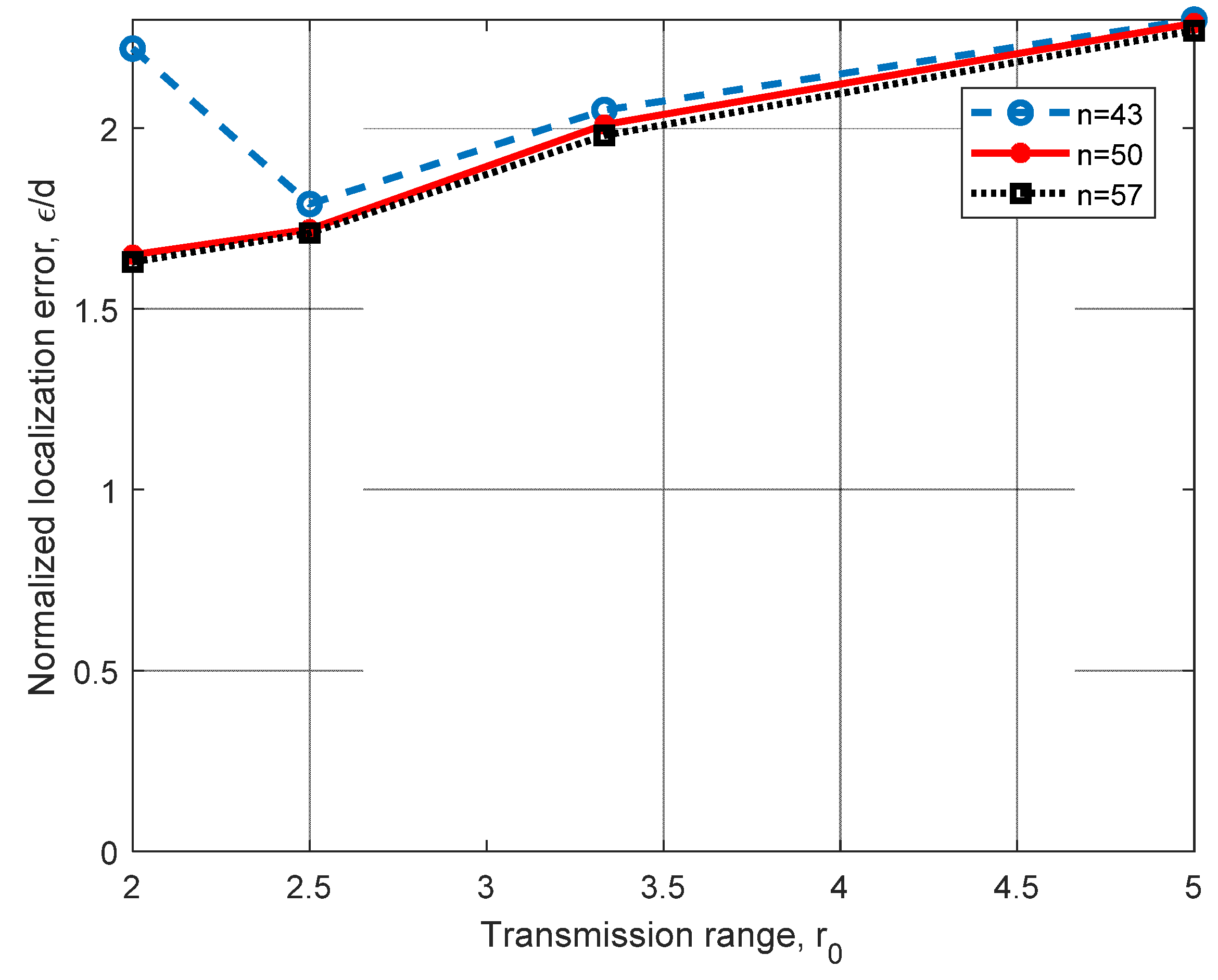
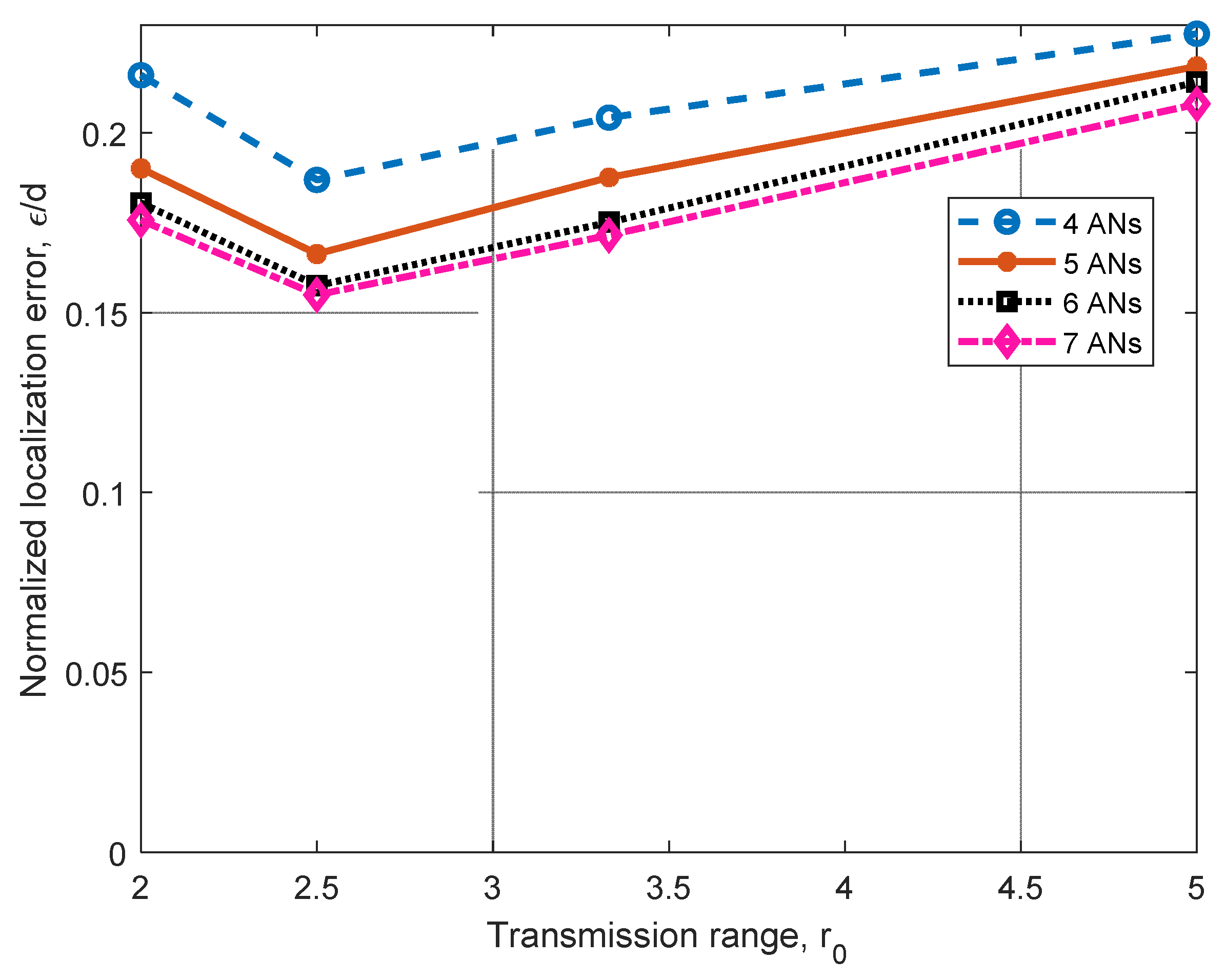
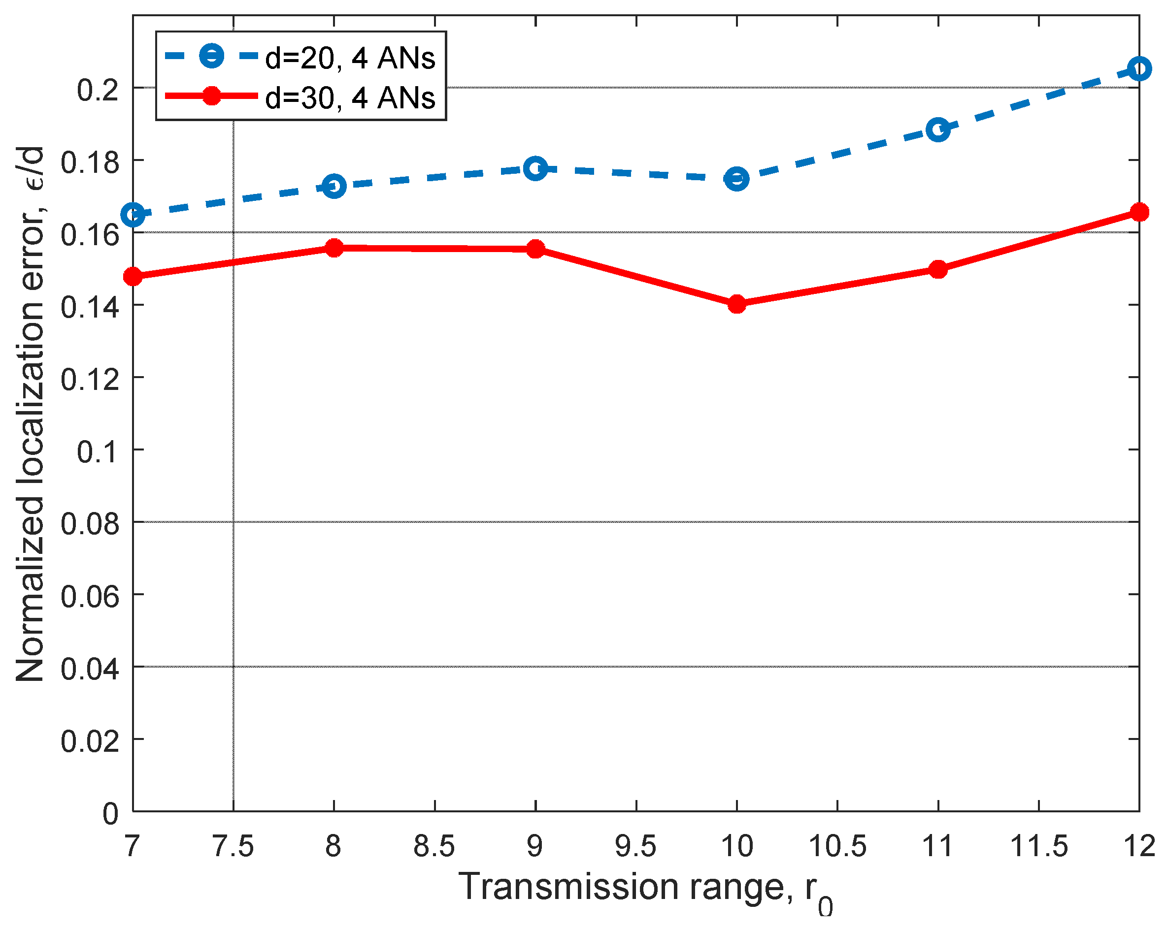
4.2. The 3D Evaluation

Let us consider a 3D scenario defined by a regular tetrahedron, as illustrated in Figure 5a, having four ANs with coordinates AN₁(0,0,0), AN₂(d,0,0), AN₃(d cos$\frac{\pi }{3}$, d sin$\frac{\pi }{3}$,0), and AN₄($\frac{d}{2}$,$\frac{d}{2}$tan$\frac{\pi }{6}$,d). Routes from ANs to node n₀ are obtained according to Dijkstra’s routing algorithm [19]. As stated before, the estimated distance between AN_i and node n₀, Δ_{i, (j,k,l)} is approximated by the number of hops in the route connecting them. In addition, the maximum coverage radius is initially set to r₀ = 2 m, and the number of nodes in the network is set as follows: for the 2D scenario, we randomly deploy 70 to 90 nodes in a dxd square meter area, and as the working area is a triangle defined by ANs coordinates, the proportional number of nodes within the triangle is n = 30 to 40 nodes. For the 3D scenario, 300 to 400 nodes are also randomly deployed in a dxdxd cube meter volume, and as the working space is a tetrahedron defined by ANs coordinates, the proportional number of nodes in such tetrahedron is n = 43 to 57.

For the 3D assessment, we extended the variety of scenarios analyzed, varying more network conditions (ANs locations, coverage radius r₀, and the number of nodes) and under different values of the space discretization unit L. Note that L defines the vertices v_j,k,l on the discretized space and thus the searching points related to distances ${\delta }_{i,(j,k,l)},$ in Equation (2).

Figure 7 shows the performance of the relational searching method for a 3D scenario, as shown in Figure 5a, with AN₁(0,0,0), AN₂(d,0,0), AN₃(d cos$\frac{\pi }{3}$, d sin$\frac{\pi }{3}$,0) and AN₄($\frac{d}{2}$,$\frac{d}{2}$tan$\frac{\pi }{6}$,d), where d = 10 m. In this figure, we analyzed the performance of the method under different coverage ranges, r₀, and the number of nodes n in the working space. In this analysis, we can observe that as r₀ increases, the normalized error ε/d increases; however, the Euclidean quadratic error ε shows stability, as it remains close to 2 m. In this figure, we can also observe that by increasing the number of nodes in the space, we can achieve a significant improvement for r₀ = 2 m. This is because better routes can be found if more nodes are in the network, and this is more significant when r₀ is small. Even that the transmission range r₀ is selected in the range r₀ = [2 m 5 m] for the following evaluations, it can be larger than 5 m; however, the normalized localization error is very close to that obtained for r₀ = 5 m. Simulations were performed for r₀ = 6 m, 7 m, 8 m and n = 43 nodes, obtaining ε/d = 0.2236, 0.2235 and 0.2526, showing error saturation, which is a desirable behavior.

Figure 7. Error analysis for different numbers of nodes n in the network and different transmission ranges, r₀, using four ANs in a 3D scenario, with d = 10 m.

In Figure 8, results from a different perspective are shown; on the x-axis, the average Euclidean quadratic distance error ε (m) is presented, and on the y-axis, the values of the cumulative distribution function describing the percentage of cases when ε is under a given distance are presented.

Figure 8. Quadratic error CDF analysis for different transmission ranges, r₀, and n = 43, using four ANs in a 3D scenario.

Simulations in Figure 8 were performed for a 3D scenario with four ANs, (n = 43, L = 1). Note that results in Figure 8 are not normalized to d. In this analysis, we can observe that for r₀ = 2.5 m, approximately 100% of the calculations are under 3 m of error. The worst analyzed case is when r₀ = 2 m, which can be explained because distance estimations from anchors to the n₀ are based on the hop count, and for a very small r₀, we achieve longer routes, resulting in bad distance estimations. However, this can be alleviated by increasing the number of nodes in the space, as previously observed in Figure 7. From these results, we can infer that the best hop distance estimation is achieved for r₀ = 2.5 m. We can also infer that for r₀ < 2.5 m, the distance might be overestimated, and for r₀ > 2.5 m, the distance might be underestimated.

In practice, it is difficult to guarantee uniform deployment of ANs, as in Figure 5a. Therefore, evaluations were carried out for regular and non-regular scenarios. Simulations were conducted for different shapes of the tetrahedron base, and the results obtained were similar to those reported in Figure 7 and Figure 8. These results are presented in Table 3. Note that moving only AN₃ coordinates gives enough variability to the scenario setup, as the tetrahedron’s base is changed. In these simulations, coordinate x₃ was varied, and coordinate y₃ was fixed in order to keep the same tetrahedron volume to keep the comparison fair. Simulation parameters were set as n = 43, d = 10 m, AN₁(0,0,0), AN₂(d,0,0), AN₃(x₃, d sin$\frac{\pi }{3}$, 0), AN₄($\frac{d}{2}$,$\frac{d}{2}$tan$\frac{\pi }{6}$, h), and h = 10 m.

Table 3. Error (ε/d) analysis for different tetrahedron bases (“x” coordinate of AN₃).

r0(m)	2	2.5	3.333	5
x3 = d sin$\frac{\pi }{3}$	0.2160	0.1869	0.2042	0.2275
x3 = d sin$\frac{\pi }{3}$ ± 1	0.2129	0.1899	0.2080	0.2364
x3 = d sin$\frac{\pi }{3}$ ± 2	0.2232	0.2067	0.2157	0.2269
x3 = d sin$\frac{\pi }{3}$ ± 3	0.2160	0.1821	0.1997	0.2370
x3 = d sin$\frac{\pi }{3}$ ± 4	0.2106	0.1879	0.1927	0.2273
x3 = d sin$\frac{\pi }{3}$ ± 5	0.2128	0.2025	0.2082	0.2286

However, when the tetrahedron height h is increased, we observe a slight degradation of the proposed PL method, which is due to the increased size of the searching space. In Table 4, these results are presented for different transmission ranges, n = 43, d = 10 m and AN₁(0,0,0), AN₂(d,0,0), AN₃(d cos$\frac{\pi }{3}$, d sin$\frac{\pi }{3}$, 0), AN₄($\frac{d}{2}$,$\frac{d}{2}$tan$\frac{\pi }{6}$, h). Note that the proposed method shows robustness under volume increments; that is, for a volume increment of 30% (from h = 10 m to h = 13 m), the normalized error ε/d increment ranges from 3.5% to 17%.

Table 4. Error (ε/d) analysis for different tetrahedron (4 ANs) heights h and transmission ranges r₀.

r0(m)	2	2.5	3.333	5
h = 10 m	0.216	0.1869	0.204213	0.2275
h = 11 m	0.224	0.196075	0.218312	0.262
h = 12 m	0.23	0.2002	0.220778	0.2623
h = 13 m	0.22356	0.193516	0.233377	0.2672

In Figure 9, we analyzed the localization method for different values of the discretization unit L. As we anticipated, a finer discretization grid helps to reduce the normalized error ε/d significantly. In this figure, we can observe that when the discretization unit is decreased to L = $\frac{1}{2}$ m, improvements ranging from 39% to 45% can be achieved. As we continue to decrease L, ε/d diminishes in a lower proportion. With this analysis, we demonstrate that a finer discretization leads to a lower distance error (close to 1 m) for L = $\frac{1}{2}$ m, and to 0.8 m for L = $\frac{1}{3}$ m.

Figure 9. Error analysis for different values of the discretization unit L and different transmission ranges r₀, using four ANs in a 3D scenario, for d = h = 10 m.

However, as we decreased the discretization step L, we increased the number of vertices in the searching space, increasing the uncertainty. In Table 5, we analyzed the entropy function for the 3D scenario illustrated in Figure 5a, for L = 1 m and L = $\frac{1}{2}$ m. The entropy values for L = 1 m and L = 1/2 m without the proposed method on the discretized space are H_L=1 = 5.04 and H_L=1/2 = 6.9735, respectively. Note that the method helps to significantly decrease the uncertainty.

Table 5. Entropy analysis for 4 ANs with different transmission ranges, r₀, and discretization unit L.

r0(m)	2	2.5	3.333	5
HL=1	2.8	2.66	2.86	3.04
HL=1/2	4.94	4.7112	4.78	5.29

In Figure 10, we present the performance comparison for a 3D scenario with four to seven ANs. This analysis was carried out for n = 43 randomly deployed nodes in the tetrahedron illustrated in Figure 5b, with AN₁ to AN₄ deployed as stated before and AN₅, AN₆, AN₇ deployed at the centroid of planes conformed by the corresponding sets (AN₁, AN₂, AN₃), (AN₂, AN₃, AN₄), and (AN₁, AN₂, AN₄), with d = 10. As anticipated, when we increase from 4 ANs to 5 ANs, we can see improvements from approximately 5% to 12% for all the cases reported. Additionally, when we increase from 5 ANs to 6 ANs, improvements from 2% to 6.6% are achieved. Finally, when we increase from 6 ANs to 7 ANs, improvements from 1.6% to 2.84% are observed. Simulations were performed by moving AN₅ on the plane conformed by the set (AN₁, AN₂, AN₃), and it was observed that the achieved improvement decreases as the AN₅ approaches AN₁, AN₂, or AN₃. A similar experiment was conducted regarding AN₆ and AN₇, and similar behavior was observed. For these scenarios, the entropy was also calculated, and results were very similar to those reported in Table 4 for L = 1. Note that when the number of ANs increases, there is an improvement in the location. However, for a given reachability ratio r₀, the further increase in the number of ANs provides marginal improvement.

Figure 10. Error (ε/d) analysis for different transmission ranges r₀ for four to seven ANs with L = 1.

Thus far, we have focused on evaluations for indoor scenarios, which are frequently used on Industry 4.0 applications. However, there are some applications in smart industries and sensor networks in which outdoor environments have to be considered. Since the proposed relational positioning method does not rely on range estimation, there is no need to consider signal impairments associated with outdoor scenarios. However, the scenario size d, as well as the transmission range r0, have to be increased in order to assess outdoor networks. As shown in Figure 11, we evaluated the performance of the relational positioning method for d = 20 m, 30 m, and for transmission ranges r₀ from 6 m to 12 m for the basic set up, n = 43, L = 1, and regular deployment of ANs (AN₁(0,0,0), AN₂(d,0,0), AN₃(d cos$\frac{\pi }{3}$, d sin$\frac{\pi }{3}$,0) and AN₄($\frac{d}{2}$,$\frac{d}{2}$tan$\frac{\pi }{6}$,d)). Results in Figure 11 show that the estimation error does not grow in the same proportion as the size of the network d, as maximal estimation errors for d = 20 m and d = 30 m are in the order of 4.1 m and 4.9 m, respectively, for r₀ = 12 m. Note that as stated before, finer discretization, as well as additional ANs, can help to improve the location estimation.

Figure 11. Error (ε/d) analysis for different transmission ranges, r₀, in outdoor deployment.

It is important to observe that as the method relies on the routes connecting ANs to n₀, better route algorithms might help to obtain better positioning estimations. Note that proactive routing protocols might render better positioning estimations, as routes are updated periodically. However, reactive (on-demand) routing algorithms might lead to large positioning errors if the location estimation is calculated based on old routing data.

5. Conclusions

A position location-searching method suitable for both 2D and 3D sensor networks and based on relative distance relationships was proposed. This method can be used for indoor and outdoor scenarios, and it was demonstrated that its accuracy can be improved without the need to increase the infrastructure requirements. Since in Industry 4.0, traditional indoor and outdoor localization methods are not suitable due to the lack of reliability of distance estimation, the proposed method provides a reliable alternative to solve the need for position location information. The proposed method is robust, as it does not rely on the goodness of estimated distances. Its performance was assessed for multi-hop environments using a low-cost distance estimation method (hop count) considering several ANs for 3D networks. The 3D PL searching method is based on the space discretization once the searching space has been defined and enclosed by a set of ANs and on a vertex weight assignment due to distance relations. It was shown through simulations that the PL searching method improves as we increase the number of ANs in the operational area/space. However, using only four ANs combined with a small discretization step (L = $\frac{1}{3}$ m) is sufficient to achieve the best performance reported. Additionally, marginal improvements can be achieved when the number of nodes in the network increases, as better routes and therefore better distance estimations become available.

References

1. Syberfeldt, A.; Ayani, M.; Holm, M.; Wang, L.; Lindgren-Brewster, R. Localizing Operators in the Smart Factory: A Review of Existing Techniques and Systems. In Proceedings of the ISFA2016, Cleveland, OH, USA, 1–3 August 2016. [Google Scholar]
2. Pahlavan, K.; Krishnamurthy, P. Principles of Wireless Networks: A Unified Approach, 1st ed.; Prentice Hall PTR: Upper Saddle River, NJ, USA, 2002. [Google Scholar]
3. Yavari, M.; Nickerson, B.G. Ultra-Wideband Wireless Positioning Systems; Tech. Rep. TR14-230; Faculty of Computer Science, University of New Brunswick: Fredericton, NB, Canada, 2014. [Google Scholar]
4. Muñoz-Rodriguez, D.; Bouchereau, F.; Vargas-Rosales, C.; Enriquez-Caldera, R. Position Location Techniques and Applications, 1st ed.; Academic Press: Cambridge, MA, USA, 2009. [Google Scholar]
5. Jin, M.H.; Wu, H.K.; Hormg, J.T. An Intelligent Handoff Scheme Based on Location Prediction Technologies. IEEE Eur. Wirel. 2002, 551–557. [Google Scholar]
6. Yash, A.; Kritika, J.; Orkun, K. Smart vehicle monitoring and assistance using cloud computing in vehicular Ad Hoc networks. Int. J. Transp. Sci. Technol. 2018, 7, 60–73. [Google Scholar]
7. Villalpando-Hernandez, R.; Munoz-Rodriguez, D.; Vargas-Rosales, C.; Rizo-Dominguez, L. 3-D Position Location in Ad Hoc Networks: A Manhattanized Space. IEEE Commun. Lett. 2017, 21, 124–127. [Google Scholar] [CrossRef]
8. Sayed, A.H.; Tarighat, A.; Khajehnouri, N. Network-based wireless location: Challenges faced in developing techniques for accurate wireless location information. IEEE Signal Process. Mag. 2005, 22, 24–40. [Google Scholar] [CrossRef]
9. Vargas-Rosales, C.; Maidana, Y.; Villalpando-Hernandez, R.; Azpilicueta, L. Statistical Evaluation of the Positioning Error in Sequential Localization Techniques for Sensor Networks. In Proceedings of the 3rd International Electronic Conference on Sensors and Applications ECSA2016, Copenhagen, Denmark, 28 November–2 December 2016. [Google Scholar]
10. Singh, M.; Khilar, P.M. An Analytical Geometric Range Free Localization Scheme Based on Mobile Beacon Points in Wireless Sensor Network. Wirel. Netw. 2016, 22, 2537–2550. [Google Scholar] [CrossRef]
11. Brena, R.F.; García-Vazquez, J.P.; Galván-Tejada, C.E.; Muñoz-Rodriguez, D.; Vargas-Rosales, C.; Fangmeyer, J., Jr. Evolution of Indoor Positioning Technologies: A Survey. J. Sens. 2017, 2017, 2630413. [Google Scholar] [CrossRef]
12. Zafari, F.; Gkelias, A.; Leung, K. A Survey of Indoor Localization Systems and Technologies. IEEE Commun. Surv. Tutor. 2019, 21, 2568–2599. [Google Scholar] [CrossRef] [Green Version]
13. Kim, E.; Choi, E. A 3DAd Hoc Localization System Using Aerial Sensor Nodes. IEEE Sens. J. 2015, 15, 3716–3723. [Google Scholar] [CrossRef]
14. Xu, Y.; Zhuang, Y.; Gu, J. An improved 3D Localization Algorithm for the Wireless Sensor Networks. Int. J. Distrib. Sens. Netw. 2015, 11, 315714. [Google Scholar] [CrossRef] [PubMed]
15. Yang, X.; Yan, F.; Liu, J. 3D Localization Algorithm Based on Voronoi Diagram and Rank Sequence in Wireless Sensor Network. Sci. Program. J. 2017, 2017, 4769710. [Google Scholar] [CrossRef] [Green Version]
16. Nath, S.; Venkatesan, N.E.; Kumar, A.; Kumar, V. Theory and Algorithms for Hop-Count-Based Localization with Random Geometric Graph Models of Dense Sensor Networks. ACM Trans. Sens. Netw. 2012, 8, 1–38. [Google Scholar] [CrossRef]
17. Saeed, N.; Nam, H.; Al-Naffouri, T.; Alouini, M. A State-of-the-Art Survey on Multidimensional Scaling-Based Localization Technique. IEEE Commun. Surv. Tutor. 2019, 21, 3565–3583. [Google Scholar] [CrossRef] [Green Version]
18. Tao, J.; Tao, R.; Buehrer, M. Collaborative Position Location for Wireless Networks Using Iterative Parallel Projection Method. In Proceedings of the IEEE Globecom, Miami, FL, USA, 6–10 December 2010. [Google Scholar]
19. Tommiska, M.; Skytta, J. Dijkstra’s Shortest Path Routing Algorithm in Reconfigurable Hardware. In Proceedings of the 11th Conference on Field-Programmable Logic Applications, Belfast, UK, 27–29 August 2001; pp. 653–657. [Google Scholar]
Publisher’s Note: MDPI stays neutral with regard to jurisdictional claims in published maps and institutional affiliations.
Article Metrics
Citations
Article Access Statistics
Multiple requests from the same IP address are counted as one view.