Towards Robust Representations of Spatial Networks Using Graph Neural Networks

Abstract

The effectiveness of a machine learning model is impacted by the data representation used. Consequently, it is crucial to investigate robust representations for efficient machine learning methods. In this paper, we explore the link between data representations and model performance for inference tasks on spatial networks. We argue that representations which explicitly encode the relations between spatial entities would improve model performance. Specifically, we consider homogeneous and heterogeneous representations of spatial networks. We recognise that the expressive nature of the heterogeneous representation may benefit spatial networks and could improve model performance on certain tasks. Thus, we carry out an empirical study using Graph Neural Network models for two inference tasks on spatial networks. Our results demonstrate that heterogeneous representations improves model performance for down-stream inference tasks on spatial networks.

1. Introduction

The representation of any data fed to a machine learning model impacts the usefulness of that data [1]. The model cannot learn what it cannot see and a data representation will present its perspective of the data to the model [2].

A spatial network is defined as a network where the nodes and edges are spatial entities with a metric imposed on them [3]. Examples of spatial networks include street networks, rail networks, social networks. Spatial networks can be described through representations for a machine learning task. A type of representation is the homogeneous graph representation (we use the terms data representation and graph representation interchangeably). A homogeneous graph representation is defined as one where there is only one node and edge type in the graph [4]. For example, we can describe a street network using a homogeneous graph representation. Here, the graph nodes will denote street segments and the graph edges will denote adjacency or intersection. Nonetheless, homogeneous graph representations fail to capture the multi-type nature of spatial networks. Typically, spatial networks exist as a combination of objects with mixed types and relations. For example, the street network will exist alongside other spatial entities such as buildings or water bodies. We can address this limitation by describing spatial networks using heterogeneous graph representations. A heterogeneous graph representation is defined as one where there is at least two types of nodes or edges in the graph [4]. Thus, a heterogeneous graph representation offers a rich perspective of the data by describing the multi-type nature of spatial networks [4].

Machine learning models perform better when the choice of representation captures the explanatory factors of variation behind the data [2]. This is particularly important for spatial networks where entities exhibit inter-dependence. Let us take for example, a heterogeneous graph representation of a spatial network describing streets and buildings, where the nodes are street segments or buildings and the edges are spatial relations. 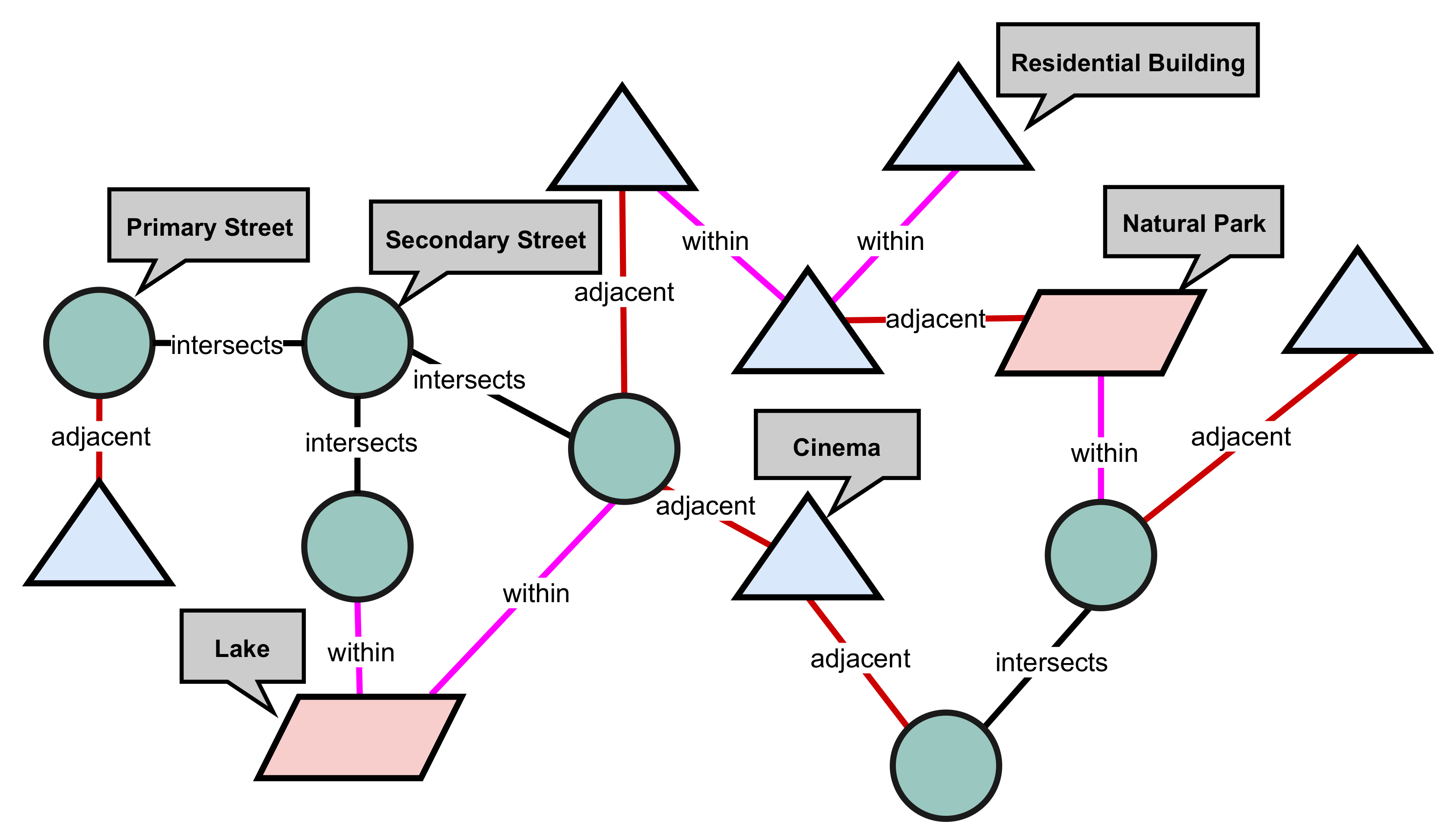There is a higher likelihood of a node being a residential building if it is sufficiently connected to one or more residential streets [5,6]. Intuitively, residential streets are likely to be constructed near or around residential buildings. From the machine learning models’ perspective, this is a better representation and could improve model performance. It follows then that the heterogeneous graph representation could improve model performance for machine learning tasks on spatial networks. See Figure 1 for an illustration of the heterogeneous graph representation of a spatial network.

Graph Neural Networks (GNNs) are a type of artificial neural network that is designed to learn directly on graphs. In contrast to traditional machine learning methods which are designed to work on structured data, GNNs are capable of embedding both the relational and contextual information about spatial elements during the learning process [7,8]. However, many applications of GNNs to spatial problems have been on homogeneous graph representations [8]. This may be due to the fact that deriving the homogeneous data representation typically only involves retrieving the physical representation [8]. Compared to deriving the heterogeneous graph representation which could easily be non-trivial, e.g., due to an arbitrary number of possible relations. We are of the opinion that learning on heterogeneous graph representations of spatial networks is an important direction, especially within the context of GNNs. Describing spatial entities closer to their true state using heterogeneous graph representations could present insights into the model that would otherwise be ignored. We posit that heterogeneous graph representations could improve model performance for spatial networks. Consequently, we adopt the GNN paradigm of learning for our experiments.

While advances in machine learning techniques and a proliferation of spatial data have benefited Geo-AI efforts in solving many inference tasks, there have been concerns about the robustness of general models versus specialised models for Geo-AI. Studies have shown that specialised models for spatial tasks usually perform better than general models for spatial data [8,9]. For example, Aodha et al. [10] demonstrate that encoding the geographical location as a probability prior improves the model performance of off-the-shelf fine-grained image classifiers. Similarly, Chu et al. [11] who show that leveraging geographical information could significantly improve model performance for image classifiers in resource-constrained environments. Yan et al. [12] develop mathematical embeddings for places using spatial context which outperforms mainstream embeddings. This begs the question: What defines a specialised model for spatial data? We adopt the definition by Goodchild [13] which outlines the following criteria to identify a specialised model for spatial data.

1.

Invariance test—the model results should vary across space.

2.

Representation test—the model should contain spatial representations.

3.

Formulation test—the model formulation should use spatial concepts.

4.

Outcome test—the model inputs and outputs should differ.

A model is said to be specialised for spatial data if it meets at least one of the four criteria. It is important to mention that equal importance is assumed for all the criteria. In this article, we focus on criteria 2—the representation test.

In this article, we study the link between data representations and the performance of machine learning models on spatial problems. Fundamentally, we seek to understand the impact of data representations on model performance. We focus on Graph Neural Network models for the problem of semantic inference on spatial networks. Spatial semantics can be defined as the descriptions or meanings of spatial objects, such as the type of a street, the use of a building. The process of predicting these semantics is referred to as semantic inference. We formulate two semantic inference tasks to guide our study: inference of street types and inference of building types (Section 3). These tasks are formulated specially to address the semantic inference problem on OpenStreetMap [5]. We propose an approach to derive heterogeneous graph representations from spatial entities of different types (Section 4). We develop this approach into a reusable code package called HetSpatial. Then, we develop a neural network framework for transductive learning on heterogeneous graph representations to address the inference tasks (Section 5). Similarly, we train models for the homogeneous graph representations using state of the art GNN methods. We compare the performance for models trained using the heterogeneous graph representation and homogeneous graphs representations. Our evaluations show model improvements of up to 40% average F-score using heterogeneous graph representations and 20% average F-score using homogeneous graph representations. To the best of our knowledge, this is the first attempt to empirically measure the impact of representations on model performance for spatial tasks. We release the code and data used for our experiments. The deepening integration of artificial intelligence and geographical information science vis-à-vis Geo-AI demands investigation into the efficient development of prediction models. We believe that our contributions in this paper will benefit Geo-AI by offering insights on the impact of representations on model performance for geo-spatial data [9,13]. Efficiently integrating multiple data sources for inference have been identified as one of the challenges of Geo-AI [14]. Towards this, heterogeneous representations could be a promising solution, e.g., for multi-modal learning, hybrid forms of spatial networks (socio-spatial networks) described using heterogeneous representations [15,16].

2. Background

Our study seeks to address the semantic inference problem in spatial networks. We discuss machine learning approaches to this problem. Corcoran et al. [6] attempt to predict the semantics of streets on OpenStreetMap using the street geometries. They focus on inferring street types, using geometric properties such as length and linearity. The street segments are modelled as graphs and a Markov random field model is used to perform inference. They use data from Boston, achieving 68% precision and 65% recall on the classification tasks. Iddianoze and McArdle [5] develop machine learning models using contextual information to predict the semantics of streets on OpenStreetMap. They define contextual information as the type of objects that lie within the neighbourhood of a street. Similarly, they focus on street types as the semantics of the streets. They train tree-based models to perform inference. Bonafilia et al. [17] developed both weakly-supervised and semi-supervised machine learning models for building maps. They focus on building detection and road segmentation. Their models achieve improved performance by using data collected from OpenStreetMap. Iddianozie and McArdle [7] proposed the use of transfer learning to develop transferable models to mitigate the data availability problem for enriching spatial semantics. Using a statistical multi-measure, they are able to determine apriori the suitability of a model for a domain.

Our work in this article focuses on Graph Neural Networks (GNNs) which are a type of Artificial Neural Networks designed to work on graphs. GNNs can be broadly classified into spectral and spatial approaches. Spectral GNNs derive object representations through operations on the graph Laplacian matrix, which could be very expensive to compute, thereby affecting scalability [18,19,20,21]. Spatial GNNs derive representations directly from the graph, operating on spatially close neighbours of a graph object [22,23]. Graph Neural Networks (GNNs) are capable of encoding the relational inductive bias in structures, hereby addressing a limitation of standard machine learning methods [7,9,24,25]. This capability has been leveraged to improve model performance. He et al. [26] proposed a hybrid neural architecture that is comprised of a Convolutional Neural Network (CNNs) and a Graph Neural Network (GNN). Their architecture is targeted at inferring the attributes of street networks. Their evaluations show that incorporating the GNN allows their architecture to mitigate the receptive field limitation of CNNs. Iddianozie and McArdle [8] develop effective Graph Neural Network models to infer spatial semantics using a node importance sampling technique. Their technique enables the GNN to outperform vanilla GNNs on the street semantics inference task. However, they focus on homogeneous graph representations, whereas, heterogeneous graph representations could offer a richer representation of data and improve model performance [4]. Our work in this article extends the applications of GNNs to the semantic inference of spatial networks using heterogeneous graph representations. We can also classify Graph Neural Networks based on the type of graph representations they are designed to work on as: Homogeneous Graph Neural Networks and Heterogeneous Graph Neural Networks. Similar to our earlier definitions of homogeneous and heterogeneous graph representations, a graph neural network is said to be homogeneous if it is designed to work on homogeneous graph representations and heterogeneous if it is designed to work on heterogeneous graph representations. GCN [19], GAT [23], GraphSAGE [22] are some examples of Homogeneous GNNs while HetGCN [27] and HAN [28] are some examples of Heterogeneous GNNs. We study both homogeneous and heterogeneous GNNs in this paper, in order to understand the relationship between model performance and data representations.

3. Preamble

We define important concepts in this section.

Table 1. Notations and definitions.

Notation	Definition
$\mathcal{G}=(\mathcal{V},\mathcal{E})$	A graph representation
$\mathcal{V}$	set of nodes in $\mathcal{G}$
$\mathcal{E}$	set of edges in $\mathcal{G}$
$\mathcal{P}$	semantic path
${\mathcal{D}}_{\mathcal{G}}$	the network schema of $\mathcal{G}$
$\left|\mathcal{V}\right|$	number of nodes in $\mathcal{G}$
$\left|\mathcal{A}\right|$	number of node types in $\mathcal{G}$
$\left|\mathcal{R}\right|$	number of relation types in $\mathcal{G}$
$\mathbf{h}$	node representation
$\mathcal{Y}$	set of class labels for nodes in $\mathcal{G}$
$\mathcal{N}\left(v\right)$	Neighbourhood of a node v

outlines notations and their definitions.

Definition 1.

Spatial Entity: A spatial entity $\mathcal{S}=(\mathcal{M},\mathcal{N})$ is defined as an object that is embedded in space, where $\mathcal{M}$ is a set of geo-coordinates that defines its bounds or location in space and $\mathcal{N}$ is a set of real-valued features that describes $\mathcal{S}$.

Definition 2.

Graph Representation: We define a graph representation as $\mathcal{G}=(\mathcal{V},\mathcal{E})$, where $\mathcal{V}$ and $\mathcal{E}$ denote the object set and relation set, respectively. The objects are mapped to types based on a function $\phi :\mathcal{V}\to \mathcal{A}$, the relations are mapped to types based on a function $\psi :\mathcal{E}\to \mathcal{R}$. Thehomogeneousgraph representation is one where $\left|\mathcal{A}\right|=1$ and $\left|\mathcal{R}\right|=1$ and theheterogeneousgraph representation is one where where $\left|\mathcal{A}\right|+\left|\mathcal{R}\right|>2$.

Definition 3.

Semantic Path: A semantic path $\mathcal{P}$ is a path on an instance of a graph representation $\mathcal{G}$, denoted in the form $A_1\stackrel{R_1}{\to }{A}_2\stackrel{R_2}{\to }\cdots \stackrel{R_l}{\to }{A}_{l+1}$, that defines a composite relation $R=R_1\circ R_2\circ \cdots \circ R_l$ between graph objects $A_1,A_2,\cdots ,A_{l+1}$ where ∘ denotes the composition operator on relations.

Definition 4.

Network Schema: A network schema ${\mathcal{D}}_{\mathcal{G}}$ defines the object and relational constraints for a graph representation $\mathcal{G}=(\mathcal{V},\mathcal{E})$ which is a directed graph representation where the objects are mapped to types as $\phi :\mathcal{V}\to \mathcal{A}$ and the relations are mapped to types as $\psi :\mathcal{E}\to \mathcal{R}$. A graph representation defined by a network schema is called an instance of that network schema.

3.1. Graph Neural Networks

Graph neural networks are designed to learn a representation $\mathbf{h}$ for the nodes of a graph using the node and edge connectivity. $\mathbf{h}$ is computed for a node $v\in \mathcal{G}$ by an incremental update using the aggregations of the neighbours of v. The neighbours are defined as the nodes within the k-hop neighbourhood of v. The representation of a node v at the k-th layer of the GNN can be defined as:

$${\mathbf{h}}_v^k={\mathrm{COMBINE}}^k\left({\mathbf{h}}_v^{k-1},{\mathrm{AGGREGATE}}^k\left(\left\{\left({\mathbf{h}}_v^{k-1},{\mathbf{h}}_u^{k-1},e_{uv}\right)\forall u\in \mathcal{N}\left(v\right)\right\}\right)\right)$$

where ${\mathbf{h}}_v^k$ is the representation of a node v at the k-th layer, $e_{uv}$ is the attribute vector and $\mathcal{N}\left(v\right)$ is the set of nodes within the k-hop neighbourhood of v.

Problem Definition

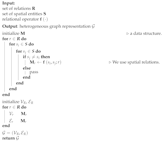
Our problem definition is two-fold. Firstly, given a set of spatial elements presented in any generic format. We seek to derive graph representations for these elements. In this article, we derive both homogeneous and heterogeneous graph representation as stated in Definition 2. Secondly, we seek to infer the object types $\mathcal{A}$ in $\mathcal{G}$. Recall that the object type mapping is defined by the function $\phi$. The labels of $\mathcal{V}$ is given by $\mathcal{Y}=\{y_1,\cdots ,y_c\}\in {\mathbb{R}}^c$, where c is the number of class labels that we consider for that particular instance of $\mathcal{G}$. In this article, we focus on inferring object types. The objective of the second problem is to develop a function $\mathcal{F}\left(·\right)$ which given a graph representation $\mathcal{G}$, supervisedly learns the mapping between $\mathcal{V}$ and $\mathcal{Y}$.

4. Methods

4.1. Constructing Heterogeneous Graph Representations

The heterogeneous graph representations is a graph representation with more than one node type and/or edge type. Given a set of spatial elements with their spatial coordinates, we define the edge relations between spatial elements using known spatial relations such as intersects and within-x distance. In Figure 2, we present an abstraction of the heterogeneity in spatial networks. Note that in this paper, we focus on streets and buildings which is depicted accordingly in Figure 1.

In this article, we consider a heterogeneous graph representation as a directed graph representation. We follow the traditional definitions of concepts from graph theory. See

Table 2. Graph theory concepts and definitions.

Concept	Definition
Adjacent nodes	The nodes of a graph representation are adjacent if an edge connects them.
Incidence	A node and an edge of a graph are incident if the edge connects the node to another node.
Node degree	The number of edges incident to the node.
Directed graph	A graph representation is said to be directed if the edges have a direction.
Connected graph	A graph representation is said to be connected if all of its nodes can be accessed from any other node.

for a definition of graph concepts used in this article. Our focus is on deriving heterogeneous spatial representations for spatial elements. There are two challenges that need to be discussed. The first challenge is the difference between the physical representations of spatial elements and general network representation as defined by graph theory. We define the physical representations of spatial elements as the convention used for storing the elements in ubiquitous systems and geo-spatial data stores such as maps. Within the context of spatial elements, while certain types of spatial elements are physically represented as networks, others are not. Street networks are an example of spatial networks that usually are physically represented as networks. Because their physical representation follows the network conventions of graph theory, there is little to no additional overhead required to derive their graph representation. In this case, the graph representation of a street network could be one where the nodes are street segments and the edges indicate adjacency between the street segments. Other elements such as buildings and natural bodies are not necessarily represented physically as networks. Hence, at the very least, deriving their graph representations requires a scoping of the relations to be considered.

The second challenge is that there exists an arbitrary number of spatial elements and relations that could be considered. Bear in mind that the spatial elements to be considered while deriving a graphical representation should be beneficial to the task at hand. For example, when trying to build a model that infers the type of a street as residential, encoding the relation between that street and other buildings (where the type of the building could be encoded as a node feature) may be beneficial to the model than say its relation to bus stations [5]. Similarly, the type of relations we can define on spatial entities varies widely. For example, we could encode the relation between buildings using spatial measures such as euclidean distance between buildings or buildings that share the same age range or buildings whose household income fall in the same range. It could be said then that the type of relations considered in a heterogeneous graph representation depends on the task at hand.

Ultimately, we want to be able to generate representations for spatial entities that strikes a balance between adequate representation of the real-life perspective and suitability to the task at hand. In this article, we implement a new package that derives the heterogeneous graph representation for a place. We call this package HetSpatial. The package uses a place name and a set of relations to derive the heterogeneous graph representation for that place. At this time, HetSpatial supports streets and buildings as spatial entities and uses spatial relations to encode relations between the entities. The package is developed in the python programming language. We provide the algorithm that describes at a high level how the package works in Algorithm 1, where $\mathbf{S}$ refers to a set of homogeneous spatial entities which could be presented in a generic format such as a table, $\mathbf{R}$ is the set of relations to be considered, our implementation considers spatial relations.

Algorithm 1: Derive Heterogeneous Graph Representation

Computational Complexity

The run-time and memory complexity of Algorithm 1 is $\mathcal{O}\left(\right|\mathbf{R}|\ast (\left|\mathbf{S}\right|\ast \left|\mathbf{S}\right|-1\left)\right)$, where $\left|\mathbf{S}\right|$ is the number of homogeneous spatial entities being considered and $\left|\mathbf{R}\right|$ is the number of relations.

4.2. Learning on Heterogeneous Graph Representations of Spatial Networks

The neural architecture for learning on a heterogeneous graph representation is different from that of a homogeneous graph representation. We discuss pertinent aspects of the architectural differences and describe a suitable architecture.

4.2.1. Graph Structure

The heterogeneous graph representation is one that has different types of nodes and edges. Training this representation using a neural model, we need to consider that there could be differences between the characteristics of the node and edge attributes such as the size and meaning. For example, with the node type street, we may consider the length and width of the street segment as input features, whereas, for buildings, we may consider the age of the building, number of levels, area as input features. The number of node classes being inferred could vary across node types. Hence, the problem will be to design an architecture that is able to efficiently handle these intricacies that exist in heterogeneous graph representations [28]. We discuss a suitable neural architecture in Section 4.2.3.

4.2.2. Modelling Semantics

Similar to the difference imposed by the heterogeneity of the node and edge types on the graph structure representation, the heterogeneous representations of the spatial networks deals with different semantic types. In heterogeneous graphs, we can explain semantic relations using semantic paths. A semantic path is a relation connecting objects. To illustrate, given two relations: intersects and within, a semantic path between two streets could be street—intersects →street, a path between a building and a street could be building—within→streets. When the semantic path traverses more than two objects, we may refer to it as a meta-path. Now, given the different paths or meta-paths present in a graph, we can see that certain paths will be better suited for certain tasks. For example, if we seek to infer the street type, it may be the case that the street—intersects→street path will be better suited than the building—within→ streets path. It then raises the question, how do we determine the best suited semantic path for a particular task. The attention mechanism has been used in many machine learning approaches [23,28]. We use the attention mechanism in our neural architecture to compute importance values for the semantic paths with respect to a learning task. We now describe the architecture of the neural model.

4.2.3. Neural Architecture

The neural architecture we use in this article is hierarchical, learning on the graph structure using the semantic paths [23,28]. In order to differentiate between the node types during learning for a particular task, we define a transformation matrix Q to enable a projection of nodes to a different feature space based on their type. We describe this in Equation (1).

$${\mathbf{h}}_i^{\prime }={\mathbf{Q}}_{\mathcal{P}i}·{\mathbf{h}}_i$$

(1)

Here, ${\mathbf{h}}_i$ refers to the original feature of node i and ${\mathbf{h}}_i^{\prime }$ is the embedding derived for the same node. Next, we employ the concept of attention in [23] to assign importance to a node. In essence, given a node pair $(i,j)$ connected, we can learn how important either nodes will be to each other. Due to the heterogeneous nature of the graph, the importance of node i to node j may not be the same as the importance of node j to node i. Hence, this is the non-symmetric nature of heterogeneous graphs. We define the attention $\left(a\right)$ between two nodes $(i,j)$ as

$$e_{ij}^{\mathcal{P}}=a({\mathbf{h}}_i^{\prime },{\mathbf{h}}_j^{\prime }).$$

(2)

During training, we only calculate $e_{ij}$ for nodes $j\in {\mathcal{N}}_i$, where ${\mathcal{N}}_i$ refers to the neighbourhood of node i. We use the softmax activation function to normalize the attention values between node pairs to obtain the weight coefficient ${\alpha }_{ij}^{\mathcal{P}}$

$${\alpha }_{ij}^{\mathcal{P}}=softma{x}_j\left(e_{ij}^{\mathcal{P}}\right)=\frac{\exp \left(\sigma \left({\mathrm{a}}_{\mathcal{P}}^T·[{\mathbf{h}}_i^{\prime }\parallel {\mathbf{h}}_j^{\prime }]\right)\right)}{{\sum }_{k\in {\mathcal{N}}_i^{\mathcal{P}}}\exp \left(\sigma \left({\mathrm{a}}_{\mathcal{P}}^T·[{\mathbf{h}}_i^{\prime }\parallel {\mathbf{h}}_k^{\prime }]\right)\right)}$$

(3)

In Equation (3), $\alpha$ refers to the softmax function, ${\mathrm{a}}_{\mathcal{P}}$ is the node attention vector for a semantic path $\mathcal{P}$, ${}^T$ denotes transposition, ∥ is the concatenation operator. The embedding ${\mathbf{j}}_i^{\mathcal{P}}$ for a node i from a specific semantic path $\mathcal{P}$ can be derived from its neighbourhood, thus:

$${\displaystyle {\mathbf{j}}_i^{\mathcal{P}}=\sigma \left(\sum _{j\in {\mathcal{N}}_i^{\mathcal{P}}}{\alpha }_{ij}^{\mathcal{P}}·{\mathbf{h}}_j^{\prime }\right)}$$

(4)

It has been demonstrated in [8,23] that using more than one attention head will benefit model performance and stability. We employ K attention heads in this article, we compute the node attention K times and concatenate, extending Equation (4) as follows.

$${\displaystyle {\mathbf{j}}_i^{\mathcal{P}}{=\parallel }_{k=1}^K\sigma \left(\sum _{j\in {\mathcal{N}}_i^{\mathcal{P}}}{\alpha }_{ij}^{\mathcal{P}}·{\mathbf{h}}_j^{\prime }\right)}$$

(5)

In addition to deriving the semantic-path based node embeddings, we seek to also determine embeddings for the semantic paths themselves using the attentional model. Following the proposal in [28], we define the weights for n group of semantic paths

$$({\mathrm{\Omega }}_0^{\mathcal{P}},\cdots ,{\mathrm{\Omega }}_n^{\mathcal{P}})=a({\mathbf{j}}_0^{\mathcal{P}},\cdots ,{\mathbf{j}}_n^{\mathcal{P}})$$

(6)

Here, ${\mathrm{\Omega }}^{\mathcal{P}}$ is the weights computed for a particular semantic path $\mathcal{P}$. The importance $\tau$ of each semantic path is learned by firstly transforming the node embedding $\mathbf{j}$

$${\displaystyle {\tau }_i^{\mathcal{P}}=\left(\sum _{i\in \mathcal{V}}{\mathrm{m}}^T·\tanh (\mathbf{W}·{\mathbf{j}}_i^{\mathcal{P}}+\mathbf{b})\right)·{\left|\mathcal{V}\right|}^{-1}}$$

(7)

Here, m is a vector of attention values, $\mathbf{W}$ is the weight matrix and $\mathbf{b}$ is the bias vector. We derive ${\mathrm{\Omega }}_i^{\mathcal{P}}$ from the individual semantic path importances by normalizing ${\tau }_i^{\mathcal{P}}$ using the derived importances for all semantic paths n. Hence, ${\mathrm{\Omega }}_i^{\mathcal{P}}=\mathrm{normalized}\left({\tau }_i^{\mathcal{P}}\right)$. The final node representation $\mathbf{J}$ is derived from the semantic path weights ${\mathrm{\Omega }}_i^{\mathcal{P}}$ and the node embeddings ${\mathbf{j}}_i^{\mathcal{P}}$

$${\displaystyle \mathbf{J}=\sum _{i=1}^n{\mathrm{\Omega }}_i^{\mathcal{P}}·{\mathbf{j}}_i^{\mathcal{P}}}$$

(8)

In this article, we use eight attention heads to train our model as this is shown to be stable in [8].

5. Experiments

We describe the experiments carried out for our study. The goal of our experiments was to better understand the relation between representations and model performance for spatial inference tasks.

5.1. Data

To construct the graph representations required for our experiments, we collect the spatial elements from OpenStreetMap. We use data from the following cities: Dublin, Frankfurt, Toronto, and Manchester. These cities were chosen because the semantic quality of OpenStreetMap is generally better in large cities [29]. Given that our problem is a semantic inference one, we adapt the definition of semantics from [7] as the descriptive details about spatial objects, e.g., the class of streets such as residential streets and the use of buildings such as commercial buildings on OpenStreetMap.

We construct the heterogeneous graph representations for these cities from OpenStreetMap using Algorithm 1. We consider two types of spatial objects: streets and buildings, and two types of relations: intersects and within. The intersects relation denotes a spatial intersection between two objects and the within denotes objects that lie within x distance of another object. In this article, we set x to 500 m for all representations.

The homogeneous graph representations are constructed for streets using only the intersects relation between street segments. For buildings, we use only the within relation between buildings, we set the distance to 500 m.

All the graph representations used in this article are connected graphs, in cases where there are disconnected components, we select the largest graph component for our experiments. Furthermore, we use the dual graph representation (or line graph) for our experiments. That means in all cases, the nodes are the spatial objects and the edges denote relations. For the purpose of our experiments, we generate numeric features from a normal distribution for the graph representations. We limit the size of each feature to 5. Our problem is a node classification and the node labels refer to either street types or building types. For the homogeneous case, we have separate graph representations for the street and for the buildings, whereas, for the heterogeneous case, we have one graph representation for both the streets and the buildings. We visualise the network schema for the homogeneous and heterogeneous graph representations in Figure 3. The street types considered are residential, secondary and tertiary streets. The building types are residential buildings, parking and bicycle parking. For the experiments, we train on 20%, 40%, 50% and 70% splits of the graph nodes. We use 20% and 10% of the graph nodes for the validation and testing, respectively. The same validation and test nodes are used for all the training splits. We present the number of train, validation and test nodes used in

Table 3. Data Split for the homogeneous and heterogeneous models. The train split shown here is 70% of the entire dataset.

	Train		Validation		Test
Dataset	Streets	Buildings	Streets	Buildings	Streets	Buildings
Dublin	29,253	3847	8358	1099	4179	549
Frankfurt	6794	1862	1941	532	970	266
Toronto	26,749	3691	7642	1054	3821	527
Manchester	4688	121	1339	34	669	17
(a) Homogeneous Models
Dublin	17,479	12,780	4994	3651	2497	1825
Frankfurt	10,874	2669	3107	762	1553	381
Toronto	48,659	8911	13,902	2546	6951	1273
Manchester	20,373	331	5821	94	2910	47
(b) Heterogeneous Models

. During training, we label only the training nodes in the input graph representation using a generated mask. Notice that in Table 3, there is a disparity between the number of nodes for the homogeneous and heterogeneous graph representation. This is because either graph representation is generated independently, albeit from the same domain and with different relational constraints imposed on them. The derived graph representations are provided as input to the neural network model.

5.2. Model Development

Using the embedding described in Equation (8), we are able to train a model iteratively for our heterogeneous graph representations. The input to the neural network is a graph representation with partially labelled nodes, similar to the graph in Figure 1 and the output are class predictions for the unlabelled nodes. We model the loss at each iteration using cross-entropy. The cross-entropy loss is defined

$$l=-\mathcal{Y}·\log \left({\mathcal{Y}}^{\prime }\right)$$

where $\mathcal{Y}$ is the labels for the labelled nodes, ${\mathcal{Y}}^{\prime }$ is the predicted labels for the same set of nodes derived from the embedding $\mathbf{J}$. We efficiently minimize the loss using the Adam optimization rule at each iteration [30]. We use eight attention heads in the network, a learning rate of 0.005, we set drop out for attention to 0.6 and use a regularization parameter of 0.001. The final layer of the network is fit with a softmax activation function. We train our network for 300 iterations. At each iteration, we validate our model on the validation nodes. We impose early stopping by saving the best performing model on the validation nodes, with a patience of 10 epochs. All our models are trained using PyTorch and the Deep Graph Library [31,32].

Baselines

We use three state of the art architectures to train the baseline models. These are the homogeneous graph neural networks. We implement the Graph Convolutional Network (GCN) from [19] as a 2-layer feed-forward network with 16 hidden features. The $RELU$ activation function is used for the hidden layer. We use a learning rate of $0.0001$. We implement the GraphSAGE Network from [22] as a 3-layer feed-forward network with 16 hidden features. The activation function for the hidden layers is the $RELU$. We use a learning rate of $0.001$. We implement the Graph Attention Network from [23] as a 2-layer feed-forward network with 8 hidden features, 8 attention heads and a learning rate of 0.001. The final layers of these architectures are activated using the softmax function. We train the baselines for 300 iterations. We impose early stopping by saving the best performing model on the validation nodes. An in-depth discussion of these baselines are contained in the original papers, and we direct the interested reader to them for further details.

5.3. Results

We present the results of our experiments in

Table 4. Table showing the macro F1-score results for building type inference. The values in bold and underlined represent the best and second best performing approaches for each city/split, respectively.

Dataset	Split	GCN	GAT	GraphSAGE	HetSpatial
Dublin	20%	0.33 ± 0.012	0.36 ± 0.029	0.32 ± 0.002	0.33 ± 0.010
	40%	0.33 ± 0.014	0.40 ± 0.031	0.34 ± 0.050	0.33 ± 0.004
	50%	0.57 ± 0.045	0.57 ± 0.037	0.32 ± 0.002	0.33 ± 0.007
	70%	0.33 ± 0.011	0.54 ± 0.047	0.39 ± 0.063	0.33 ± 0.007
Frankfurt	20%	0.50 ± 0.018	0.51 ± 0.019	0.47 ± 0.014	0.41 ± 0.010
	40%	0.49 ± 0.025	0.50 ± 0.030	0.45 ± 0.006	0.41 ± 0.008
	50%	0.49 ± 0.029	0.52 ± 0.030	0.45 ± 0.005	0.41 ± 0.012
	70%	0.50 ± 0.026	0.48 ± 0.024	0.47 ± 0.022	0.41 ± 0.007
Toronto	20%	0.65 ± 0.035	0.49 ± 0.014	0.48 ± 0.002	0.49 ± 0.001
	40%	0.62 ± 0.027	0.51 ± 0.020	0.48 ± 0.003	0.49 ± 0.002
	50%	0.66 ± 0.020	0.47 ± 0.013	0.48 ± 0.003	0.49 ± 0.001
	70%	0.63 ± 0.028	0.48 ± 0.002	0.48 ± 0.002	0.49 ± 0.002
Manchester	20%	0.50 ± 0.225	0.36 ± 0.080	0.40 ± 0.163	0.42 ± 0.028
	40%	0.36 ± 0.080	0.58 ± 0.234	0.42 ± 0.162	0.42 ± 0.022
	50%	0.74 ± 0.227	0.52 ± 0.215	0.73 ± 0.250	0.41 ± 0.019
	70%	0.58 ± 0.252	0.74 ± 0.254	0.49 ± 0.199	0.41 ± 0.027

,

Table 5. Table showing the macro F1-score results for street type inference. The values in bold and underlined represent the best and second best performing approaches for each city/split, respectively.

Dataset	Split	GCN	GAT	GraphSAGE	HetSpatial
Dublin	20%	0.29 ± 0.001	0.32 ± 0.006	0.29 ± 0.001	0.56 ± 0.348
	40%	0.29 ± 0.001	0.31 ± 0.005	0.29 ± 0.002	0.64 ± 0.345
	50%	0.29 ± 0.001	0.32 ± 0.007	0.29 ± 0.002	0.52 ± 0.333
	70%	0.29 ± 0.003	0.31 ± 0.004	0.29 ± 0.001	0.58 ± 0.290
Frankfurt	20%	0.29 ± 0.008	0.33 ± 0.012	0.28 ± 0.004	0.52 ± 0.300
	40%	0.28 ± 0.003	0.33 ± 0.018	0.28 ± 0.003	0.55 ± 0.307
	50%	0.28 ± 0.003	0.33 ± 0.015	0.28 ± 0.003	0.60 ± 0.310
	70%	0.28 ± 0.003	0.34 ± 0.013	0.28 ± 0.003	0.50 ± 0.281
Toronto	20%	0.30 ± 0.005	0.32 ± 0.005	0.27 ± 0.002	0.32 ± 0.087
	40%	0.29 ± 0.004	0.29 ± 0.003	0.27 ± 0.003	0.36 ± 0.081
	50%	0.28 ± 0.004	0.31 ± 0.007	0.27 ± 0.002	0.33 ± 0.101
	70%	0.27 ± 0.002	0.30 ± 0.007	0.27 ± 0.002	0.33 ± 0.179
Manchester	20%	0.32 ± 0.013	0.34 ± 0.021	0.31 ± 0.007	0.75 ± 0.313
	40%	0.31 ± 0.002	0.31 ± 0.012	0.31 ± 0.002	0.65 ± 0.329
	50%	0.31 ± 0.007	0.32 ± 0.013	0.30 ± 0.003	0.78 ± 0.317
	70%	0.31 ± 0.006	0.35 ± 0.020	0.30 ± 0.003	0.62 ± 0.373

,

Table 6. Table showing the micro F1-score results for building type inference. The values in bold and underlined represent the best and second best performing approaches for each city/split, respectively.

Dataset	Split	GCN	GAT	GraphSAGE	HetSpatial
Dublin	20%	0.92 ± 0.013	0.94 ± 0.013	0.93 ± 0.011	0.93 ± 0.007
	40%	0.93 ± 0.010	0.94 ± 0.008	0.93 ± 0.009	0.93 ± 0.006
	50%	0.95 ± 0.008	0.96 ± 0.008	0.93 ± 0.009	0.93 ± 0.005
	70%	0.92 ± 0.012	0.95 ± 0.008	0.93 ± 0.009	0.93 ± 0.004
Frankfurt	20%	0.73 ± 0.023	0.80 ± 0.013	0.81 ± 0.023	0.69 ± 0.02
	40%	0.77 ± 0.022	0.80 ± 0.02	0.82 ± 0.021	0.69 ± 0.024
	50%	0.74 ± 0.031	0.81 ± 0.028	0.82 ± 0.017	0.70 ± 0.026
	70%	0.75 ± 0.020	0.83 ± 0.025	0.82 ± 0.017	0.70 ± 0.018
Toronto	20%	0.90 ± 0.013	0.91 ± 0.011	0.92 ± 0.009	0.96 ± 0.006
	40%	0.87 ± 0.013	0.86 ± 0.016	0.93 ± 0.012	0.96 ± 0.006
	50%	0.89 ± 0.014	0.84 ± 0.014	0.92 ± 0.012	0.96 ± 0.005
	70%	0.86 ± 0.016	0.92 ± 0.009	0.93 ± 0.009	0.96 ± 0.007
Manchester	20%	0.86 ± 0.078	0.84 ± 0.064	0.87 ± 0.077	0.73 ± 0.085
	40%	0.85 ± 0.076	0.90 ± 0.072	0.85 ± 0.077	0.71 ± 0.066
	50%	0.95 ± 0.040	0.90 ± 0.070	0.94 ± 0.058	0.71 ± 0.057
	70%	0.90 ± 0.088	0.94 ± 0.064	0.86 ± 0.075	0.70 ± 0.074

and

Table 7. Table showing the micro F1-score results for street type inference. The values in bold and underlined represent the best and second best performing approaches for each city/split, respectively.

Dataset	Split	GCN	GAT	GraphSAGE	HetSpatial
Dublin	20%	0.75 ± 0.005	0.62 ± 0.008	0.75 ± 0.005	0.72 ± 0.180
	40%	0.75 ± 0.006	0.59 ± 0.008	0.75 ± 0.009	0.79 ± 0.247
	50%	0.75 ± 0.006	0.58 ± 0.008	0.75 ± 0.007	0.70 ± 0.251
	70%	0.74 ± 0.006	0.62 ± 0.006	0.75 ± 0.006	0.78 ± 0.180
Frankfurt	20%	0.71 ± 0.013	0.57 ± 0.013	0.73 ± 0.017	0.72 ± 0.180
	40%	0.73 ± 0.010	0.59 ± 0.021	0.73 ± 0.013	0.75 ± 0.199
	50%	0.72 ± 0.012	0.62 ± 0.013	0.73 ± 0.012	0.78 ± 0.213
	70%	0.73 ± 0.016	0.61 ± 0.011	0.73 ± 0.015	0.71 ± 0.247
Toronto	20%	0.62 ± 0.006	0.52 ± 0.008	0.67 ± 0.009	0.70 ± 0.121
	40%	0.64 ± 0.006	0.64 ± 0.007	0.67 ± 0.008	0.73 ± 0.113
	50%	0.65 ± 0.006	0.55 ± 0.009	0.67 ± 0.008	0.68 ± 0.151
	70%	0.67 ± 0.007	0.57 ± 0.009	0.67 ± 0.006	0.66 ± 0.153
Manchester	20%	0.81 ± 0.017	0.74 ± 0.02	0.84 ± 0.016	0.85 ± 0.202
	40%	0.85 ± 0.011	0.84 ± 0.013	0.84 ± 0.011	0.78 ± 0.224
	50%	0.83 ± 0.013	0.67 ± 0.016	0.84 ± 0.013	0.85 ± 0.229
	70%	0.84 ± 0.014	0.67 ± 0.014	0.84 ± 0.013	0.73 ± 0.298

. We use the macro and micro F1-score to evaluate the model performance. The macro F1-score treats all classes equally irrespective of size, whereas the micro F1-score gives uniform importance to each sample making the macro F1-score better suited for showing the effects of class imbalance. The results shown are the average scores over 20 runs on the test sets, we also show the standard deviation alongside. The best results for each case are in bold and second-best results are underlined. The columns GCN, GAT, GraphSAGE are the results for the homogeneous models which also serve as the baselines. The HetSpatial column is the result for the heterogeneous model. The split column indicates the size of training data used for the particular model. We make the following observations from the results.

• In Table 4, which refers to the macro F1-score for building type inference, the results are not significantly impacted by the training size. Particularly for the GraphSAGE and the heterogeneous models. This provides evidence that model performance is not significantly impacted by the size of the training data for building type inference. Further, the homogeneous models seem to perform best for the building type inference task, with the heterogeneous models following closely behind.
• Table 5 refers to the macro F1-score for street type inference. The heterogeneous models perform best across all training sizes for all datasets. The homogeneous models show similar performance for all training sizes. This suggests that the homogeneous models may not benefit from an increase in training data for the task of street type inference.
• We add Table 6 and Table 7 for completeness. We observe that the models perform sufficiently well and stable in most cases. However, there is no clear benefit to the impact of train size on model performance and the homogeneous and heterogeneous models perform relatively similar with no clear winner.

Our observations demonstrate that model performance can be improved based on the data representation used. Specifically, the heterogeneous representation improves model performance for street type inference while the homogeneous representation is better suited for building type inference. To express the differences succinctly, we compute the percentage improvement derived from either the heterogeneous models or the homogeneous models using the mean macro F1-score. For the heterogeneous models, we use the mean results over the splits in Table 4 and Table 5, i.e., sum the values, divided by four. For the homogeneous models, we compute the mean results using the best performing model at each split, also from Table 4 and Table 5. The percentage improvement for the street type inference problem using the heterogeneous models is Dublin—26.0%, Frankfurt—21.0%, Toronto—3.5%, Manchester—37.0%, where the percentage improvement for the building type inference problem using the homogeneous models is Dublin—13.75% Frankfurt—9.75%, Toronto—15.0%, Manchester—22.5%. Considering class imbalance and paying attention to Table 5 which is the macro F1-score, we see a clear benefit to the heterogeneous model as it outperforms the homogeneous models for the street type inference in all cases. However, this is not the case for building type inference as seen in Table 4. We suspect that this may be as a result of the smaller number of building nodes available to the model for training compared to the number of street nodes. Perhaps, for heterogeneous representations, the size of the node types used for training could impact the inference performance for that node type. This suggests that type imbalance could be a limitation of heterogeneous graph representations. An interesting direction for future work will be to investigate the impact of type imbalance in heterogeneous graph representations to model performance. It may be that in the presence of type imbalance, using the homogeneous graph representation may be better for model performance.

6. Conclusions

In this article, we have studied the problem of data representations for the semantic inference of spatial networks using Graph Neural Networks. Based on the fact that data representations impact the performance of a machine learning model [2], we seek to explore the link between data representation and model performance. We argue that the expressive nature of heterogeneous graph representations of spatial networks offers richer structural and semantic information which may improve model performance for certain tasks than their homogeneous counterparts. We focus on street type and building type inference problems in spatial networks. Our empirical evaluations show that heterogeneous graph representations may indeed be better suited for the street type inference problem than the homogeneous graph representation.

As part of our contributions, we propose an approach to generate heterogeneous representations of spatial networks from generic representations, which we developed into a python package called HetSpatial and release for public use available on https://github.com/chiddianozie/hetspatial (accessed on 14 June 2021). Furthermore, we implement a neural architecture for learning on heterogeneous graph representations for inferring the semantics of different spatial objects. Then, we evaluate this neural architecture against homogeneous learning approaches. We release the code and datasets for our experiments. 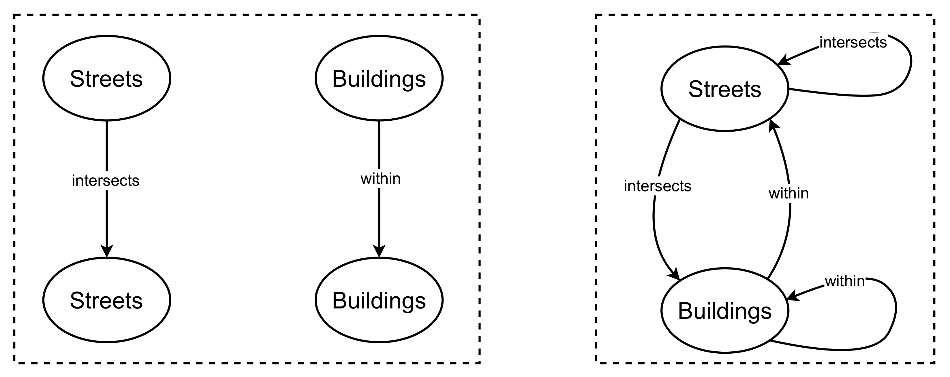For future work, we will improve the HetSpatial package to cover more spatial entities and relations, as shown in Figure 2.

Advancements in Geo-AI will benefit from a deeper understanding of specialised models for spatial data. Our work in this article contributes to this understanding by offering insight into the relationship between data representations and model performance on geo-spatial data. A promising frontier for Geo-AI is the efficient integration of multiple data sources for data-driven tasks. One example is a combination of image and textual data for inference, also known as multi-modal learning [16]. Another example is hybridizing spatial networks by interfacing them with social networks, into a type of socio-spatial network [15]. In this regard, we hope our work will inspire conviction that the expressive nature of heterogeneous representations makes them worth exploring.

References

1. Liu, Z.; Lin, Y.; Sun, M. Representation Learning for Natural Language Processing; Springer Nature: London, UK, 2020. [Google Scholar]
2. Bengio, Y.; Courville, A.; Vincent, P. Representation learning: A review and new perspectives. IEEE Trans. Pattern Anal. Mach. Intell. 2013, 35, 1798–1828. [Google Scholar] [CrossRef] [PubMed]
3. Barthélemy, M. Spatial networks. Phys. Rep. 2011, 499, 1–101. [Google Scholar] [CrossRef] [Green Version]
4. Shi, C.; Li, Y.; Zhang, J.; Sun, Y.; Philip, S.Y. A survey of heterogeneous information network analysis. IEEE Trans. Knowl. Data Eng. 2016, 29, 17–37. [Google Scholar] [CrossRef]
5. Iddianozie, C.; Bertolotto, M.; Mcardle, G. Exploring Budgeted Learning for Data-Driven Semantic Inference via Urban Functions. IEEE Access 2020, 8, 32258–32269. [Google Scholar] [CrossRef]
6. Corcoran, P.; Jilani, M.; Mooney, P.; Bertolotto, M. Inferring semantics from geometry: The case of street networks. In Proceedings of the 23rd SIGSPATIAL International Conference on Advances in Geographic Information Systems, Seattle, DC, USA, 3–6 November 2015; ACM: New York, NY, USA, 2015; p. 42. [Google Scholar]
7. Iddianozie, C.; McArdle, G. A transfer learning paradigm for spatial networks. In Proceedings of the 34th ACM/SIGAPP Symposium on Applied Computing, Limassol, Cyprus, 8–12 April 2019; pp. 659–666. [Google Scholar]
8. Iddianozie, C.; McArdle, G. Improved Graph Neural Networks for Spatial Networks Using Structure-Aware Sampling. ISPRS Int. J. Geo-Inf. 2020, 9, 674. [Google Scholar] [CrossRef]
9. Janowicz, K.; Gao, S.; McKenzie, G.; Hu, Y.; Bhaduri, B. GeoAI: Spatially Explicit Artificial Intelligence Techniques for Geographic Knowledge Discovery and Beyond; Taylor & Francis: Oxfordshire, UK, 2020. [Google Scholar]
10. Mac Aodha, O.; Cole, E.; Perona, P. Presence-only geographical priors for fine-grained image classification. In Proceedings of the IEEE/CVF International Conference on Computer Vision, Seoul, Korea, 27–28 October 2019; pp. 9596–9606. [Google Scholar]
11. Chu, G.; Potetz, B.; Wang, W.; Howard, A.; Song, Y.; Brucher, F.; Leung, T.; Adam, H. Geo-aware networks for fine-grained recognition. In Proceedings of the IEEE/CVF International Conference on Computer Vision Workshops, Seoul, Korea, 27–28 October 2019. [Google Scholar]
12. Yan, B.; Janowicz, K.; Mai, G.; Gao, S. From itdl to place2vec: Reasoning about place type similarity and relatedness by learning embeddings from augmented spatial contexts. In Proceedings of the 25th ACM SIGSPATIAL International Conference on Advances in Geographic Information Systems, Redondo Beach, CA, USA, 7–10 November 2017; pp. 1–10. [Google Scholar]
13. Goodchild, M. Issues in spatially explicit modeling. In Agent-Based Models of Land-Use and Land-Cover Change, Report and Review of an International Workshop, 4–7 October 2001; LUCC International Project Office: Louvain-la-Neuve, Belgium, 2001; pp. 13–17. [Google Scholar]
14. Hu, Y.; Gao, S.; Lunga, D.; Li, W.; Newsam, S.; Bhaduri, B. GeoAI at ACM SIGSPATIAL: Progress, challenges, and future directions. Sigspat. Spec. 2019, 11, 5–15. [Google Scholar] [CrossRef]
15. Shelton, T.; Poorthuis, A.; Zook, M. Social media and the city: Rethinking urban socio-spatial inequality using user-generated geographic information. Landsc. Urban Plan. 2015, 142, 198–211. [Google Scholar] [CrossRef]
16. Baltrušaitis, T.; Ahuja, C.; Morency, L.P. Multimodal machine learning: A survey and taxonomy. IEEE Trans. Pattern Anal. Mach. Intell. 2018, 41, 423–443. [Google Scholar] [CrossRef] [PubMed] [Green Version]
17. Bonafilia, D.; Gill, J.; Basu, S.; Yang, D. Building High Resolution Maps for Humanitarian Aid and Development with Weakly-and Semi-Supervised Learning. In Proceedings of the IEEE Conference on Computer Vision and Pattern Recognition Workshops, Long Beach, CA, USA, 16–17 June 2019; pp. 1–9. [Google Scholar]
18. Bruna, J.; Zaremba, W.; Szlam, A.; LeCun, Y. Spectral networks and locally connected networks on graphs. arXiv 2013, arXiv:1312.6203. [Google Scholar]
19. Kipf, T.N.; Welling, M. Semi-supervised classification with graph convolutional networks. arXiv 2016, arXiv:1609.02907. [Google Scholar]
20. Duvenaud, D.K.; Maclaurin, D.; Iparraguirre, J.; Bombarell, R.; Hirzel, T.; Aspuru-Guzik, A.; Adams, R.P. Convolutional networks on graphs for learning molecular fingerprints. In Proceedings of the Advances in Neural Information Processing Systems, Montreal, QC, Canada, 7–12 December 2015; pp. 2224–2232. [Google Scholar]
21. Defferrard, M.; Bresson, X.; Vandergheynst, P. Convolutional neural networks on graphs with fast localized spectral filtering. In Proceedings of the Advances in Neural Information Processing Systems, Barcelona, Spain, 5–10 December 2016; pp. 3844–3852. [Google Scholar]
22. Hamilton, W.; Ying, Z.; Leskovec, J. Inductive representation learning on large graphs. In Proceedings of the Advances in Neural Information Processing Systems, Long Beach, CA, USA, 4–9 December 2017; pp. 1024–1034. [Google Scholar]
23. Veličković, P.; Cucurull, G.; Casanova, A.; Romero, A.; Lio, P.; Bengio, Y. Graph attention networks. arXiv 2017, arXiv:1710.10903. [Google Scholar]
24. Battaglia, P.W.; Hamrick, J.B.; Bapst, V.; Sanchez-Gonzalez, A.; Zambaldi, V.; Malinowski, M.; Tacchetti, A.; Raposo, D.; Santoro, A.; Faulkner, R.; et al. Relational inductive biases, deep learning, and graph networks. arXiv 2018, arXiv:1806.01261. [Google Scholar]
25. Wu, Z.; Pan, S.; Chen, F.; Long, G.; Zhang, C.; Philip, S.Y. A comprehensive survey on graph neural networks. IEEE Trans. Neural Netw. Learn. Syst. 2020, 32, 4–24. [Google Scholar] [CrossRef] [PubMed] [Green Version]
26. He, S.; Bastani, F.; Jagwani, S.; Park, E.; Abbar, S.; Alizadeh, M.; Balakrishnan, H.; Chawla, S.; Madden, S.; Sadeghi, M.A. RoadTagger: Robust Road Attribute Inference with Graph Neural Networks. In Proceedings of the AAAI Conference on Artificial Intelligence, New York, NY, USA, 7–12 February 2020; pp. 10965–10972. [Google Scholar]
27. Schlichtkrull, M.; Kipf, T.N.; Bloem, P.; Van Den Berg, R.; Titov, I.; Welling, M. Modeling relational data with graph convolutional networks. In Proceedings of the European Semantic Web Conference, Crete, Greece, 7–13 June 2018; pp. 593–607. [Google Scholar]
28. Wang, X.; Ji, H.; Shi, C.; Wang, B.; Ye, Y.; Cui, P.; Yu, P.S. Heterogeneous graph attention network. In Proceedings of the World Wide Web Conference, San Francisco, CA, USA, 7–13 May 2019; pp. 2022–2032. [Google Scholar]
29. Haklay, M. How good is volunteered geographical information? A comparative study of OpenStreetMap and Ordnance Survey datasets. Environ. Plan. B Plan. Des. 2010, 37, 682–703. [Google Scholar] [CrossRef] [Green Version]
30. Kingma, D.P.; Ba, J. Adam: A method for stochastic optimization. arXiv 2014, arXiv:1412.6980. [Google Scholar]
31. Paszke, A.; Gross, S.; Massa, F.; Lerer, A.; Bradbury, J.; Chanan, G.; Killeen, T.; Lin, Z.; Gimelshein, N.; Antiga, L.; et al. Pytorch: An imperative style, high-performance deep learning library. arXiv 2019, arXiv:1912.01703. [Google Scholar]
32. Wang, M.; Yu, L.; Zheng, D.; Gan, Q.; Gai, Y.; Ye, Z.; Li, M.; Zhou, J.; Huang, Q.; Ma, C.; et al. Deep Graph Library: Towards Efficient and Scalable Deep Learning on Graphs. arXiv 2019, arXiv:1909.01315. [Google Scholar]
Figure 1. Figure showing a heterogeneous graph representation of spatial entities from a map. To the left is a map snippet with streets and buildings highlighted. To the right is the graph representation with the triangles representing buildings on the maps, circles representing the streets. The edges between the shapes denote some defined relation such as distance or spatial intersection. An abstract depiction of heterogeneous graph representations is shown in Figure 2.
Applsci 11 06918 g001
Figure 2. An abstract depiction of a heterogeneous graph representation of spatial entities. The triangles represents buildings, circles represents streets, parallelograms represents natural bodies. The relations between the entities is defined using relations such as the spatial within, spatial intersects, spatial adjacent.
Applsci 11 06918 g002
Figure 3. Figure showing the network schema for the homogeneous and heterogeneous graph representations used in our experiments. To the left, is the network schema of the homogeneous representations for streets and buildings. To the right, is the network schema of the heterogeneous graph representations.
Applsci 11 06918 g003