A Short-Term Prediction Model of PM_2.5 Concentration Based on Deep Learning and Mode Decomposition Methods

Abstract

Based on a set of deep learning and mode decomposition methods, a short-term prediction model for PM_2.5 concentration for Beijing city is established in this paper. An ensemble empirical mode decomposition (EEMD) algorithm is first used to decompose the original PM_2.5 timeseries to several high- to low-frequency intrinsic mode functions (IMFs). Each IMF component is then trained and predicted by a combination of three neural networks: back propagation network (BP), long short-term memory network (LSTM), and a hybrid network of a convolutional neural network (CNN) + LSTM. The results showed that both BP and LSTM are able to fit the low-frequency IMFs very well, and the total prediction errors of the summation of all IMFs are remarkably reduced from 21 g/m³ in the single BP model to 4.8 g/m³ in the EEMD + BP model. Spatial information from 143 stations surrounding Beijing city is extracted by CNN, which is then used to train the CNN+LSTM. It is found that, under extreme weather conditions of PM_2.5 < 35 g/m³ and PM_2.5 > 150 g/m³, the prediction errors of the CNN + LSTM model are improved by ~30% compared to the single LSTM model. However, the prediction of the very high-frequency IMF mode (IMF-1) remains a challenge for all neural networks, which might be due to microphysical turbulences and chaotic processes that cannot be resolved by the above-mentioned neural networks based on variable–variable relationship.

1. Introduction

Particulate matter in the air with aerodynamic diameters <2.5 μm (PM_2.5) not only threaten the quality of local atmospheric environments, but also the long-term regional and global climate [1,2,3,4,5,6]. The dynamics of the ultrafine particles, such as corrosion and weathering of materials, might impact human health, especially in megacities [7,8,9,10,11]. From previous studies, PM_2.5 concentrations can be estimated by two traditional approaches, deterministic and statistical methods [12,13,14,15,16,17,18,19,20]. The former is based on the theory of atmospheric dynamics, applying physical and chemical processes of atmospheric pollutants to establish a numerical model for prediction. Its accuracy depends on how accurate the sources of pollution, the real-time emissions and the description of the physical and chemical processes [21,22]. In contrast, the statistical method establishes the prediction models using a large number of existing historical data, based on statistical methods, such as linear regression analysis and nonlinear machine learning. Generally, statistical models are more efficient for discovering the relationship between pollutants and potential predictors, yet lack explicit description of physical mechanisms [23,24,25,26,27,28,29].

In recent years, machine learning methods have brought new tools to the prediction of PM_2.5 concentration, e.g., neural networks. Sun et al. (2013) optimized a hidden Markov model (HMM), which significantly reduced the false alarm rate of PM_2.5 concentration in Northern California [30]. Zhang et al. (2015) used a neural network to predict PM_2.5 concentration through the observations of O₃, CO, PM₁₀ and other air pollutants [25]. They found that the accuracy of the neural network model is better than multivariate regression models. A deep autoencoder (DA) and a long short-term memory (LSTM) model was used to predict PM₁₀ and PM_2.5, and both DA and LSTM models performed well [14].

Due to the complexity of the PM_2.5 variability, hybrid models with multiple neural networks have been proposed recently, which usually perform better than a single model. Xu et al. (2018) introduced a GM-ARMA hybrid model to forecast short-term PM_2.5 conditions [31]. Compared to the single GM or ARMA model, the GM-ARMA model achieved a better fitting. Huang et al. (2018) constructed a hybrid model of one-dimensional convolution and LSTM [9]. They used the PM_2.5 concentration, accumulated wind speeds and precipitation as predictors, and obtained a better prediction skill than the single LSTM model. Shi et al. (2018) combined a random forest neural network and a back-propagation (BP) neural network [21]. Zhang et al. (2020) used a CPSO-BP neural network [24]. They adopted the Chaos Particle Swarm Optimization (CPSO) algorithm to update the initial weights and thresholds of the BP neural network. Most of these studies showed that the prediction of a hybrid model is better than a single model.

One of the challenges for PM_2.5 prediction is that the forecasting errors tend to increase during heavily polluted days, which is a common problem for machine learning methods. As is known, during heavily polluted days the PM_2.5 concentrations can be influenced by multi-scale processes from hourly to annual variability, such as weather conditions, pollution sources and emissions, which presents a tough challenge for machine learning. We know that a single machine learning model can perform very well for single-frequency time sequences but is not good at learning multi-frequency sequences. In this paper, an innovative idea to solve this problem is proposed: a multi-frequency sequence of the target time series can be decomposed into a set of intrinsic mode functions (IMF). For each IMF, we can use different machine learning methods to obtain the maximal learning efficiency and, therefore, the best forecast skill. Following this protocol, we first decomposed the PM_2.5 sequence into several IMFs with low- to high-frequencies, using ensemble empirical mode decomposition (EEMD). Then, we constructed a hybrid machine learning model with multiple neural networks, and each neural network was trained individually for each IMF. By doing so, we are able to see how efficient the individual neural network component is at learning and predicting the IMFs, the sum of which stands for the original PM_2.5 sequence.

2. Data and Methods

2.1. The Source of Data

The PM_2.5 data used in this paper are from China National Environmental Monitoring Center https://quotsoft.net/air/ (accessed on 20 July 2021). The PM_2.5 concentration timeseries of Beijing city is obtained by an average of 12 stations, from 1 January 2014 to 17 November 2018. In addition, the data of 143 stations in North China (105° E–125° E, 32° N–43° N) were used in Section 3.3. The meteorological data are from http://rp5.ru (accessed on 20 July 2021), including air temperatures, dew-point temperatures, sea-level pressure, and winds.

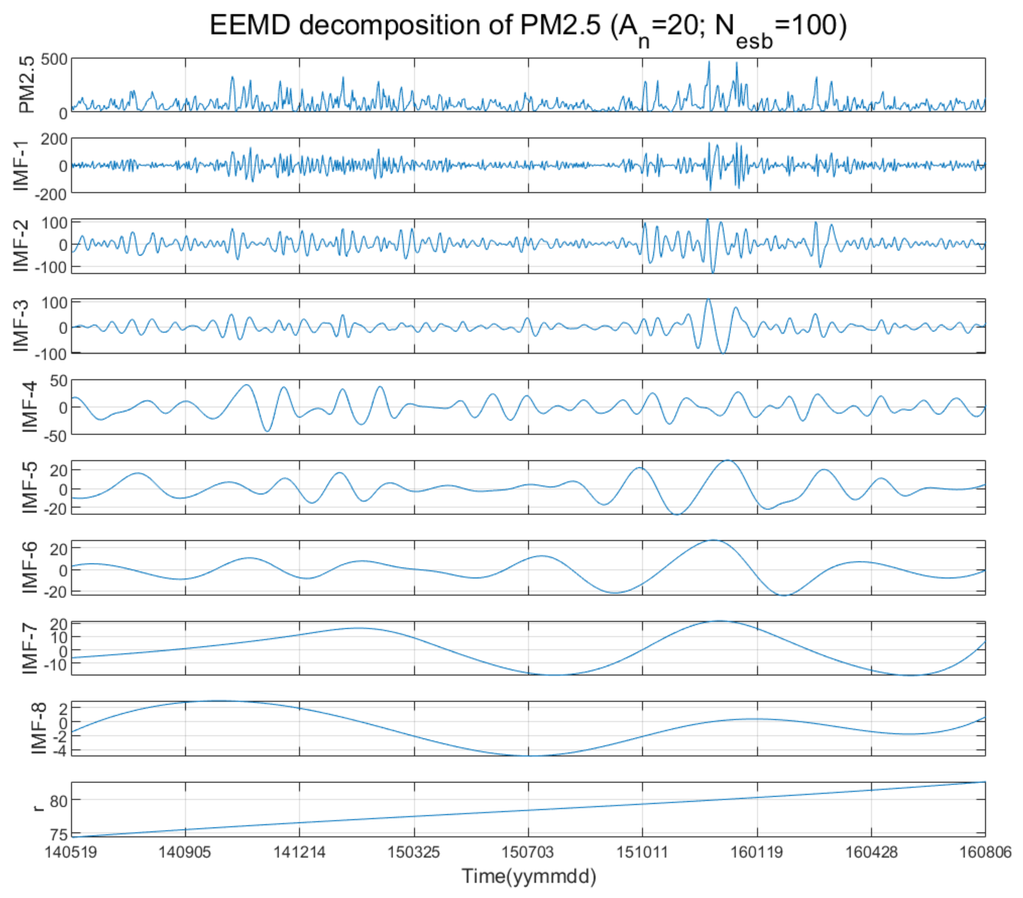
2.2. Ensemble Empirical Mode Decomposition (EEMD)

Ensemble empirical mode decomposition (EEMD) was first proposed by Wu and Huang [32]. It decomposes a timeseries of complex signals into a finite number of intrinsic mode functions (IMF). In this paper, the EEMD algorithm was used to decompose the original PM_2.5 sequence into 9 IMF components from high to low frequencies. Compared to the original PM_2.5 sequence, each IMF component contains less variability which can be trained and predicted by each neural network component. The detailed information of EEMD and its decomposition algorithm can be found in Appendix A.

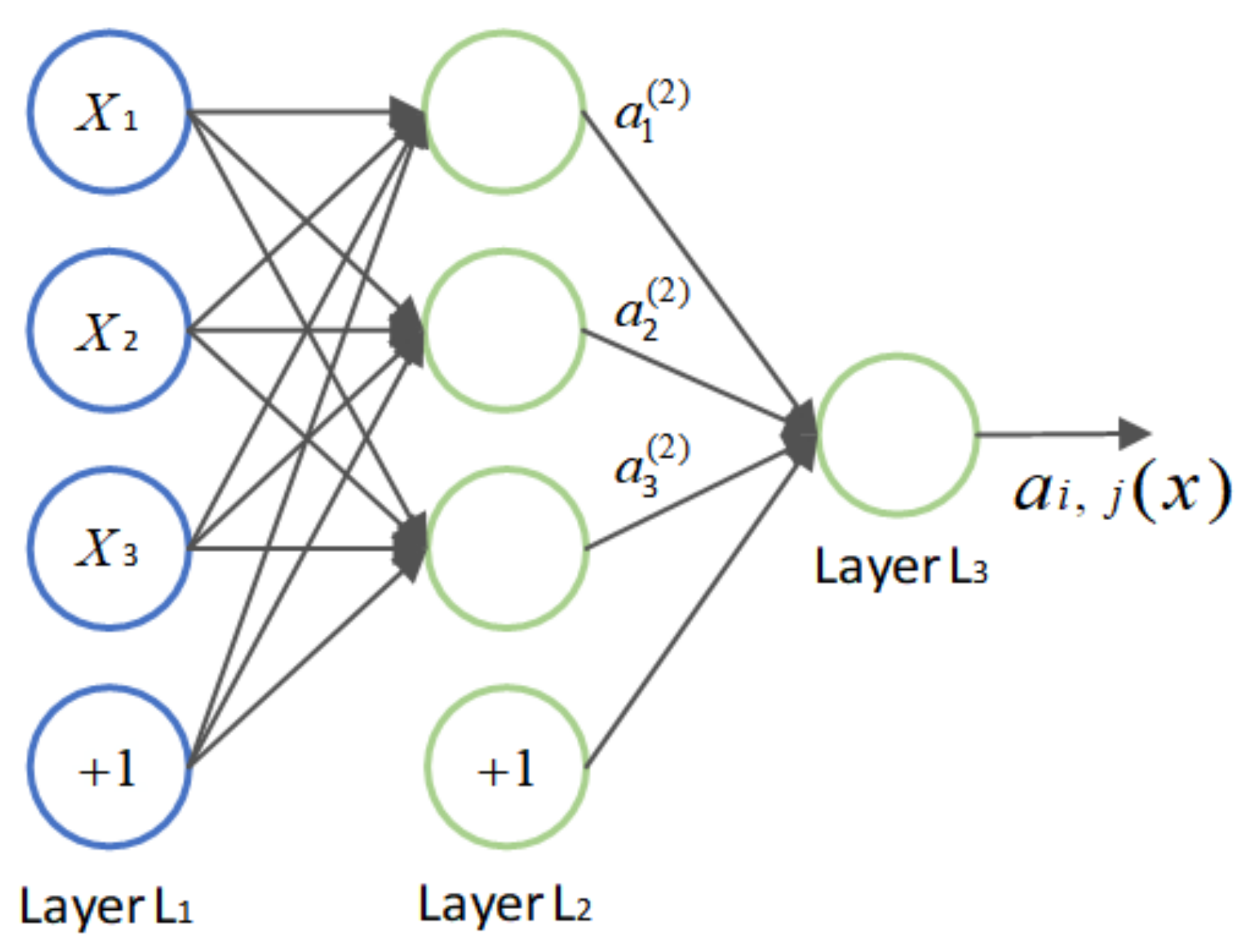
2.3. BP Neural Network

Back propagation (BP) algorithm is a supervised learning neural network, composed of one input layer, one or more hidden layers and one output layer. BP is able to produce the best fit between the input and output variables, based on back propagation of errors between truth and expected outputs from the neural network. In this study, BP neural network was used to fit the relationship between PM_2.5 concentration and meteorological variables. The detailed algorithm of BP can be found in Appendix B.

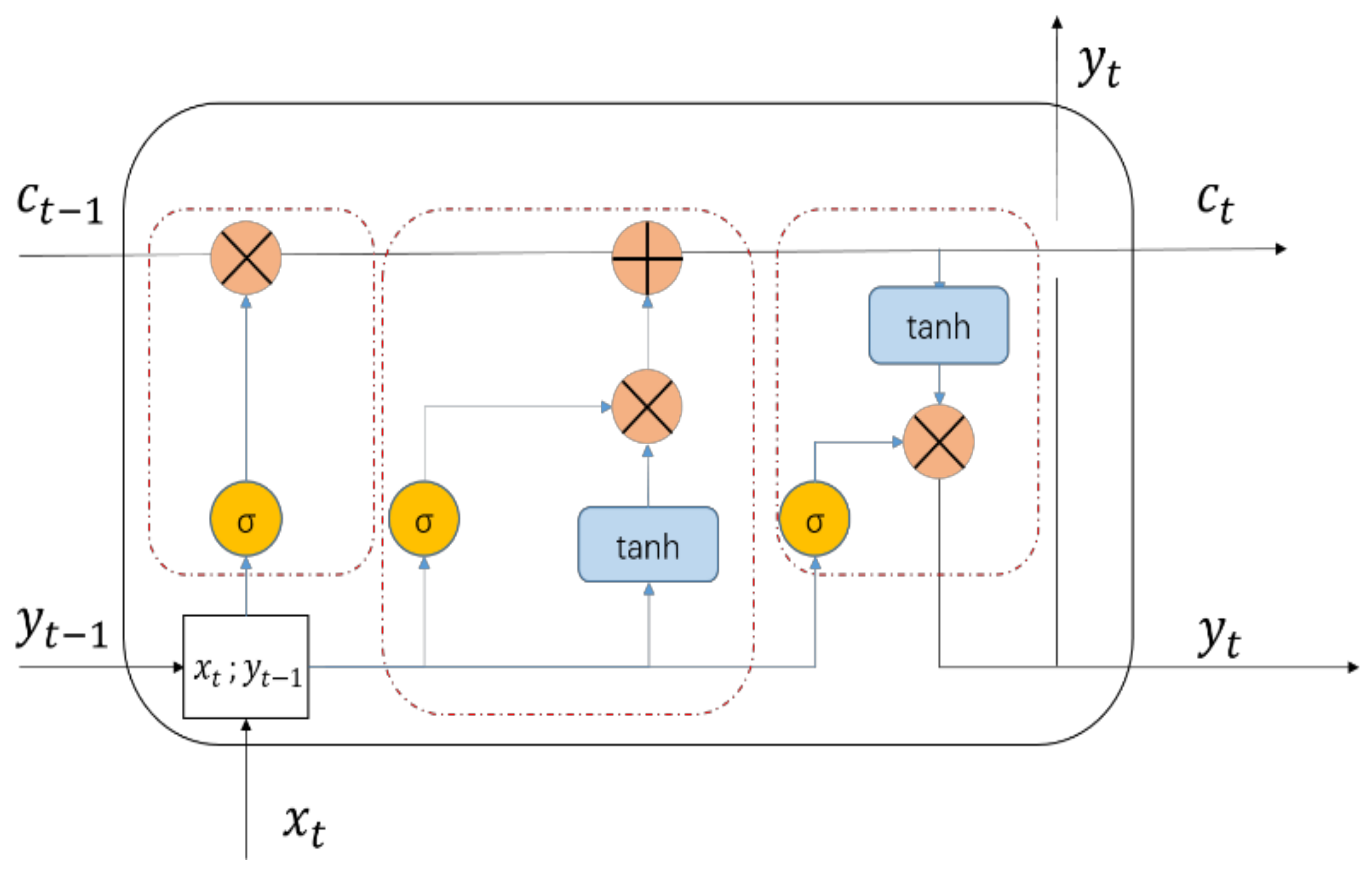
2.4. CNN-LSTM Neural Network

Convolutional neural network (CNN) is capable of extracting the spatial features of an element with its surrounding units by applying a convolutional algorithm within a certain coverage area. Long short-term memory (LSTM) is a recurrent neural network, that is able to link the present PM_2.5 to the past information of itself. Compared to the BP algorithm, LSTM does not need meteorological data to predict future PM_2.5 concentrations, but depends on the long-term correlation of the PM_2.5 sequences, which have been extensively studied by Varotsos et al. [33] for typical megacities. In this study, with the aim to explore the spatial features and the autocorrelation of the PM_2.5 timeseries, a hybrid algorithm of CNN-LSTM was used to design the prediction model for IMFs from EEMD. By doing so, the timeseries of PM_2.5 in a certain area was regarded as a 3D image, which enables CNN to capture the spatial information. Then, the extracted information from CNN was transformed into a vector in time, used by LSTM prediction. The detailed algorithm of CNN and LSTM can be found in Appendix C.

2.5. Experimental Design

PM_2.5 concentrations are associated with meteorological conditions, such as winds, temperatures, humidity, etc., and the BP neural network provides an efficient tool to fit the nonlinear PM_2.5 concentrations and the meteorological variables. On the other hand, the PM_2.5 timeseries is temporally autocorrelated and spatially correlated, especially for those low-frequency IMFs. Therefore, in this paper we designed a set of sensitivity experiments consisting of different combinations of the EEMD, BP, CNN and LSTM algorithms.

Table 1. Experimental design.

Experiment	Model	Input	Output
1	BP	M + d_PM2.5	d_PM2.5
2	EEMD+BP	M + d_PM2.5	d_PM2.5
3	LSTM	6 h_PM2.5	d_PM2.5
4	CNN+LSTM	6 h_PM2.5	d_PM2.5

Note: M = meteorological variables, d_PM_2.5 = daily PM_2.5 concentrations, 6 h_PM_2.5 = PM_2.5 concentrations at every 6 h.

shows the experimental design. Exp. 1 applies the BP to the original PM_2.5 directly. In Exp. 2, the original PM_2.5 was first decomposed by EEMD into IMFs, each of which was fit by individual BP. Summation of all IMF prediction is regarded as the output (d_PM_2.5). Exp. 3 applies LSTM to the original PM_2.5 without using meteorological variables and Exp. 4 uses a hybrid CNN+LSTM model. Note that Exp. 3 and 4 apply 6 hr PM_2.5, rather than daily PM_2.5, to explore the capability of LSTM in dealing with high-frequency timeseries.

3. Results

3.1. PM_2.5 Time-Decomposition by EEMD

Figure 1 shows the 9 IMFs decomposed from the original PM_2.5 sequence. According to their frequencies, the IMF-1,2 stand for daily to weekly variability in a time scale of 4.9 to 9.9 days, the IMF-3,4 for monthly variability (18.1 to 39.4 days), the IMF-5,6 for intra-seasonal to seasonal variability, the IMF-7,8 for annual cycles, and the IMF-9 (r) is the trend. Since the IMF-1 is obtained by subtracting IMFs 2 to 9 from the original timeseries, so that the summation of all IMFs is exactly equal to the original one; therefore, the summation of the predictions of all IMFs can be treated as the prediction for the original timeseries. One can imagine that the BP neural network can be competent for those low-frequency IMFs but will be challenged by the high-frequency IMFs. To optimize the prediction efficiency, the BP neural network is trained individually by each IMF, and thus, the network parameters and weights are different for each IMF. This is the key point that makes a mixed BP prediction model better than a single model applied directly to the original PM_2.5 timeseries, which contains full time-scale variability.

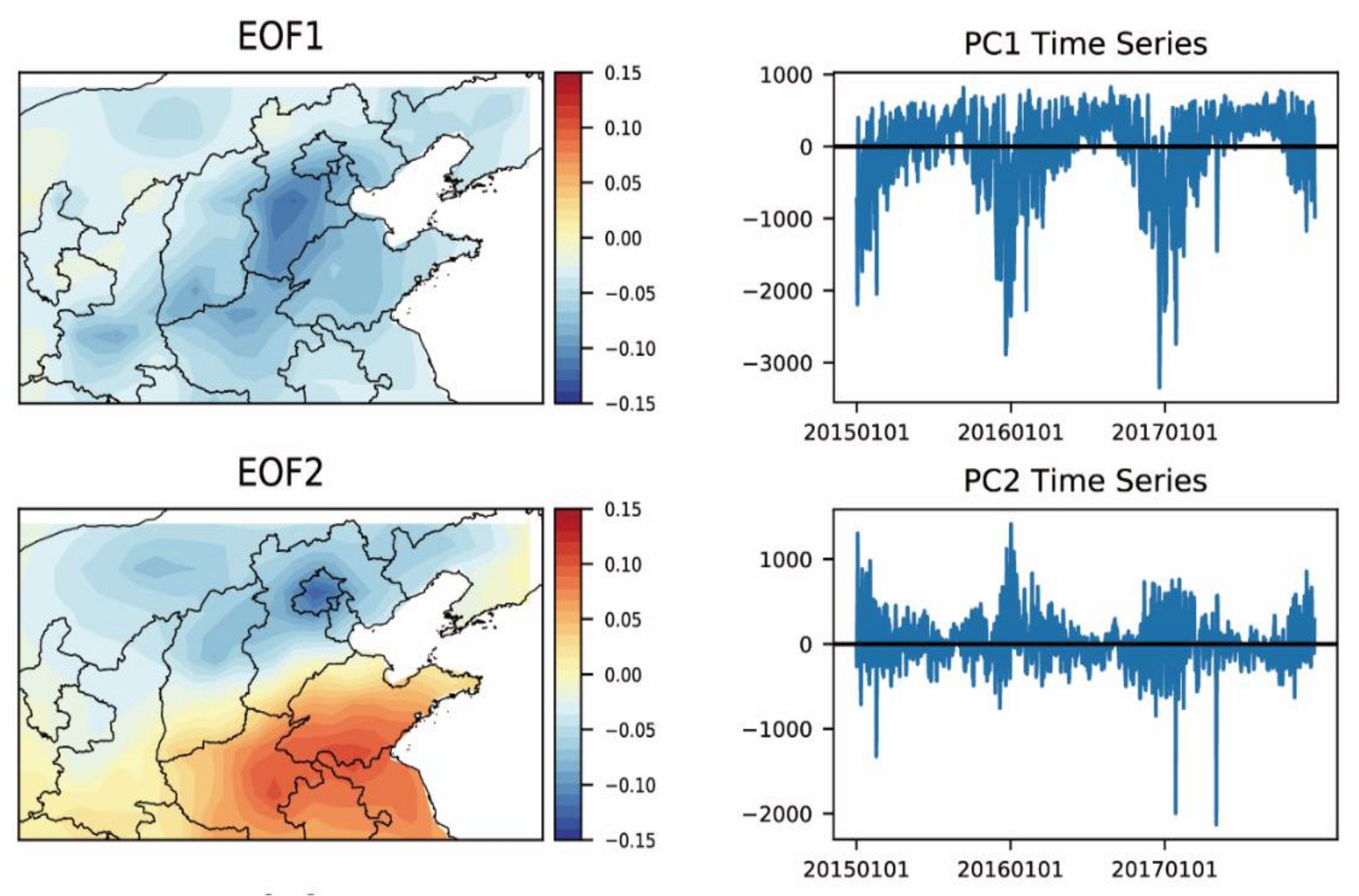
3.2. PM_2.5 Spatial Analysis by EOF

In order to demonstrate spatial features of the PM_2.5 concentration in Beijing city and the 143 stations in Northern China, an EOF analysis is applied. Due to scattering distribution of the stations, the data were interpolated to a gridded map with a resolution of 0.75° × 0.75°. Figure 2 shows the first and second modes of EOFs and PCs. The first EOF shows a PM_2.5 concentration core in Hebei province to the southwest of Beijing city, accounting for 50.2% of total variance. According to the PC1 sequence, this PM_2.5 core shows a reasonable annual cycle, reaching its maximum in winter seasons. EOF2 shows a south-to-north dipole mode, accounting for 9% of total variance. This contrasting pattern becomes prominent in winter seasons, when the overall PM_2.5 concentration of the area is high.

Figure 3 shows the time-lag correlation coefficients of Beijing and the surrounding 143 stations. The first, second and third rows show, respectively, the spatial distribution of correlation coefficient of PM_2.5 concentrations between Beijing and the surrounding areas with a 6, 12 and 24 h time lag. The left to right panels stand for low, medium and high PM_2.5 concentration scenarios. For low-concentration scenarios, we see that the PM_2.5 of Beijing is transferred from the northwest area (1st column). It indicates that the low concentration of Beijing PM_2.5 is advected by the north wind [28]. In contrast, for the high-concentration scenario in winter seasons, the PM_2.5 of Beijing outbreaks locally within Hebei province (third column).

3.3. Experimental Analyses

To assess the performance of the neural networks, we adopted the following calculations for errors and correlation coefficients: mean absolute error (MAE), root mean square error (RMSE), index of agreement (IA), determination coefficient (R²) and mean absolute percentage error (MAPE), which are defined as follows:

$$\mathrm{MAE}=\frac{1}{\mathrm{N}} {\displaystyle \sum }_{\mathrm{i}=1}^{\mathrm{N}}\left|{\mathrm{O}}_{\mathrm{i}}-{\mathrm{P}}_{\mathrm{i}}\right|$$

$$\mathrm{RMSE}=\sqrt{\frac{1}{\mathrm{N}} {\displaystyle \sum }_{\mathrm{i}=1}^{\mathrm{N}}{\left({\mathrm{O}}_{\mathrm{i}}-{\mathrm{P}}_{\mathrm{i}}\right)}^2}$$

$$\mathrm{IA}=1-\frac{{{\displaystyle \sum }}_{\mathrm{i}=1}^{\mathrm{N}}{\left({\mathrm{O}}_{\mathrm{i}}-{\mathrm{P}}_{\mathrm{i}}\right)}^2}{{{\displaystyle \sum }}_{\mathrm{i}=1}^{\mathrm{N}}{\left(\left|{\mathrm{O}}_{\mathrm{i}}-\overline{\mathrm{O}}\right|+\left|{\mathrm{P}}_{\mathrm{i}}-\overline{\mathrm{O}}\right|\right)}^2}$$

$${\mathrm{R}}^2={(\frac{1}{\mathrm{N}-1}{\displaystyle \sum }_{\mathrm{i}=1}^{\mathrm{N}}(\frac{{\mathrm{O}}_{\mathrm{i}}-\overline{\mathrm{O}}}{{\mathsf{\sigma }}_{\mathrm{O}}})(\frac{{\mathrm{P}}_{\mathrm{i}}-\overline{\mathrm{P}}}{{\mathsf{\sigma }}_{\mathrm{P}}}))}^2$$

$$\mathrm{MAPE}=\mathrm{median}\left(\left|{\mathrm{O}}_{\mathrm{i}}-\right.\left.{\mathrm{P}}_{\mathrm{i}}\right|/{\mathrm{P}}_{\mathrm{i}}\right)$$

where N is the number of samples. O and P represent the observed and predicted values. Overbar and σ represent the average and the standard deviation of corresponding variables.

In all experiments, the PM_2.5 sequence between 19 May 2014 and 31 December 2016 was used for training (90%) and testing (10%). The sequence from 1 January 2017 to 31 December 2017 was used for prediction. Figure 4 shows the wavelet spectrum of the original PM_2.5 sequence, the differences of wavelet spectrum between the original sequence and the ones trained from Exp. 1 by the BP algorithm and Exp. 2 by the EEMD+BP algorithm. Comparing Figure 4b and Figure 4c, we see that, when BP is applied directly to the original sequence (Exp. 1, Figure 4b), the errors are reduced all over the spectrum, with maximum errors between 64 to 128 days. However, if applying an EEMD decomposition before BP fitting (Exp. 2, Figure 4c), the errors can be further reduced, especially in the time period of 8 to 64 days. It indicates that individual BP training can produce an optimized fit for each IMF, especially for medium to low-frequency sequences. However, if the BP training is applied to the original sequence, although it still produces the best fit in principal, the fitting errors span the entire frequency spectrum.

Figure 5 shows the comparison of observed and predicted values for high-frequency modes (IMFs 1 and 2) and low-frequency modes (IMFs 3 to 8). For high-frequency modes, the MAE is reduced from 27.6 in Exp. 1 to 24.8 in Exp. 2. In contrast, the MAE is reduced from 21.0 to 4.8 for the low-frequency modes. Note that the R² of the Exp. 2 reaches 0.99 (Figure 5d), indicating that the individually trained BP network works perfectly for the low-frequency IMFs. However, we also see that the BP algorithm faces the same challenge in dealing with high-frequency IMFs for both Exp. 1 and 2. This is understandable, as the IMF-1 includes stochastic processes that cannot be trained by a neural network based on a variable–variable relationship.

As shown in the EOF maps in Figure 3, the PM_2.5 variability in Beijing can be affected by the surrounding area, implying that spatial information would be helpful for improving the Beijing PM_2.5 prediction. In Exp. 3, a LSTM network was applied directly to the original PM_2.5 sequence. In contrast to the BP algorithm, LSTM is able to train the PM_2.5 sequence without additional meteorological variables, as it tests the autocorrelation of the sequence itself. In Exp. 4, a CNN algorithm was used to gather the spatial information, that was then transferred to the LSTM for prediction. This is to test how spatial information can help the prediction of PM_2.5 in Beijing.

Figure 6 compares the MAEs for all experiments in five pollution levels. Comparing Exp. 1 and 2 (BP vs. EEMD-BP), the EEMD-BP network is better than the BP network for all pollution levels. This is expected, as each EEMD-decomposed IMF was trained individually by a BP network, and the low-frequency modes are perfectly fitted and predicted (Figure 5). Comparing Exp. 1 and 3 (BP vs. LSTM), we see that LSTM is worse than BP for the low-concentration level (PM_2.5 < 35), but performs better than BP for medium to high levels (PM_2.5 > 35). This implies that for high-concentration PM_2.5 sequences, its autocorrelation is stronger than its correlation with external meteorological conditions. Comparing Exp. 3 and 4 (LSTM vs. CNN-LSTM), the CNN-LSTM is better than the LSTM only in the very low (PM_2.5 < 35) and very high (PM_2.5 > 150) concentration conditions. Generally speaking, under the condition of PM_2.5 < 115, the MAEs of four neural networks are in about the same level (~20), while under the condition of PM_2.5 > 115, the hybrid models of EEMD-BP and CNN-LSTM perform better than the single BP and LSTM models.

4. Summary and Discussion

In this study, a short-term PM_2.5 concentration prediction model is established based on four deep learning neural networks (namely, EEMD, BP, CNN and LSTM). The EEMD algorithm is designed to decompose the original PM_2.5 timeseries to high- to low-frequency IMFs. Each IMF component, along with meteorological variables, is trained and predicted by three other neural networks. The summation of all IMF prediction can be treated as the prediction for the original PM_2.5 concentration. To assess the model effectiveness, we designed four sensitivity experiments and compared their MAEs in five pollution levels. It is found that the performance of a hybrid model is generally better than a single model, which is consistent with most previous studies.

To reduce the prediction errors, previous studies have investigated different combinations of neural networks to improve the structure of the prediction model [9,21,24,32]. However, the prediction of the PM_2.5 concentration in heavily polluted seasons still remains a challenge. Different from all previous studies, we assumed that a PM_2.5 timeseries in winter seasons contains full timescale variability due to complexity of weather conditions, pollution sources and emissions, which makes it really challenging for any neural network to be trained based on a limited data set. Therefore, in this study the EEMD algorithm is first used to decompose the original PM_2.5 sequence to several IMFs from high to low frequencies. Each IMF component is trained and predicted by an individual neural network. The results showed that both BP and LSTM are able to fit very well the low-frequency IMFs. Although high-frequency IMF components remain a challenge due to some chaotic processes, the total prediction errors of the summation of all IMFs are remarkably reduced.

The PM_2.5 concentration is obviously related to the surrounding area, notably Hebei province. To investigate the impact of spatial information on the PM_2.5 prediction in Beijing city, 143 stations in Northern China were used to construct a CNN-LSTM hybrid model. The results showed that, under extreme conditions of PM_2.5 < 35 and PM_2.5 > 150, the CNN-LSTM outperforms the single LSTM by ~30%. This implies that a PM_2.5 timeseries has its own temporal and spatial variability. A well-designed hybrid model on the PM_2.5 intrinsic modes and characteristics can improve its prediction skills. Regarding the very high-frequency component (IMF-1), we found that its spectrum is very similar to white noise, which might be due to microphysical processes, such as turbulence and chaotic processes, that cannot be learned by a simple neural network model. This may provide us with a new topic for future research.

References

1. Aznarte, J.L.; Siebert, N. Dynamic Line Rating Using Numerical Weather Predictions and Machine Learning: A Case Study. IEEE Trans. Power Deliv. 2017, 32, 335–343. [Google Scholar] [CrossRef]
2. Baker, K.R.; Foley, K.M. A nonlinear regression model estimating single source concentrations of primary and secondarily formed PM2.5. Atmos. Environ. 2011, 45, 3758–3767. [Google Scholar] [CrossRef]
3. Chen, Y.; Schleicher, N.; Fricker, M.; Cen, K.; Liu, X.; Kaminski, U.; Yu, Y.; Wu, X.; Norra, S. Long-term variation of black carbon and PM2.5 in Beijing, China with respect to meteorological conditions and governmental measures. Environ. Pollut. 2016, 212, 269–278. [Google Scholar] [CrossRef]
4. Chen, Y. Spatial and Temporal Variation Characteristics of PM2.5 Pollution in Autumn and Winter in Eastern Coastal Areas. J. Agric. Catastrophol. 2019, 9, 53–56. [Google Scholar]
5. Feng, X.; Li, Q.; Zhu, Y.; Hou, J.; Jin, L.; Wang, J. Artificial neural networks forecasting of PM2.5, pollution using air mass trajectory based geographic model and wavelet transformation. Atmos. Environ. 2015, 107, 118–128. [Google Scholar] [CrossRef]
6. Cracknell, A.P.; Varotsos, C.A. New aspects of global climate-dynamics research and remote sensing. Int. J. Remote Sens. 2011, 32, 579–600. [Google Scholar] [CrossRef]
7. Ferm, M.; Watt, J.; O’Hanlon, S.; De Santis, F.; Varotsos, C. Deposition measurement of particulate matter in connection with corrosion studies. Anal. Bioanal. Chem. 2006, 384, 1320–1330. [Google Scholar] [CrossRef]
8. Hrust, L.; Klaić, Z.B.; Križan, J.; Antonić, O.; Hercog, P. Neural network forecasting of air pollutants hourly concentrations using optimised temporal averages of meteorological variables and pollutant concentrations. Atmos. Environ. 2009, 43, 5588–5596. [Google Scholar] [CrossRef]
9. Huang, C.J.; Kuo, P.H. A Deep CNN-LSTM Model for Particulate Matter (PM2.5) Forecasting in Smart Cities. Sensors 2018, 18, 2220. [Google Scholar] [CrossRef] [PubMed] [Green Version]
10. Huang, F.; Li, X.; Wang, C.; Xu, Q.; Wang, W.; Luo, Y.; Tao, L.; Gao, Q.; Guo, J.; Chen, S.; et al. PM2.5 spatiotemporal variations and the relationship with meteorological factors during 2013–2014 in Beijing, China. PLoS ONE 2015, 10, e0141642. [Google Scholar]
11. Varotsos, C.; Ondov, J.; Tzanis, C.; Öztürk, F.; Nelson, M.; Ke, H.; Christodoulakis, J. An observational study of the atmospheric ultra-fine particle dynamics. Atmos. Environ. 2012, 59, 312–319. [Google Scholar] [CrossRef]
12. Huang, N.E.; Shen, Z.; Long, S.R.; Wu, M.C.; Shih, H.H.; Zheng, Q.; Yen, N.; Tung, C.C.; Liu, H.H. The Empirical Mode Decomposition and the Hilbert Spectrum for Nonlinear and Non-Stationary Time Series Analysis. Proc. Math. Phys. Eng. Sci. 1998, 454, 903–995. [Google Scholar] [CrossRef]
13. Huang, Y.; Song, F.; Liu, Q.; Li, W.; Zhang, W.; Chen, K. A bird’s eye view of the air pollution-cancer link in China. Chin. J. Cancer 2014, 33, 176–188. [Google Scholar] [CrossRef] [PubMed]
14. Jin, X.; Yang, N.; Wang, X.; Bai, Y.; Su, T.; Kong, J. Deep Hybrid Model Based on EMD with Classification by Frequency Characteristics for Long-Term Air Quality Prediction. Mathematics 2020, 8, 214. [Google Scholar] [CrossRef] [Green Version]
15. Li, S.; Xie, G.; Ren, J.; Guo, L.; Yang, Y.; Xu, X. Urban PM2.5 Concentration Prediction via Attention-Based CNN–LSTM. Appl. Sci. 2020, 10, 1953. [Google Scholar] [CrossRef] [Green Version]
16. Li, X.; Zhang, Q.; Zhang, Y.; Zheng, B.; Wang, K.; Chen, Y.; Wallington, T.J.; Han, W.; Shen, W.; Zhang, X.; et al. Source contributions of urban PM2.5 in the Beijing–Tianjin–Hebei region: Changes between 2006 and 2013 and relative impacts of emissions and meteorology. Atmos. Environ. 2015, 123, 229–239. [Google Scholar] [CrossRef] [Green Version]
17. Lv, Y.; Fu, Y.; Xin, S.G.; Wang, Y. The Harm of PM2.5 to Human Body. Liaoning Chem. Ind. 2017, 46, 618–620. [Google Scholar]
18. Nunnari, G.; Dorling, S.; Schlink, U. Modelling SO2 concentration at a point with statistical approaches. Environ. Model. Softw. 2004, 19, 887–905. [Google Scholar] [CrossRef]
19. Stern, R.; Builtjes, P.; Schaap, M.; Timmermans, R.; Vautard, R.; Hodzic, A.; Memmesheimer, M.; Feldmann, H.; Renner, E.; Wolke, R.; et al. A model inter-comparison study focussing on episodes with elevated PM10 concentrations. Atmos. Environ. 2008, 42, 4567–4588. [Google Scholar] [CrossRef]
20. Qu, Y.; Qian, X.; Song, H.; He, J.; Li, J.; Xiu, H. Machine-learning-based model and simulation analysis of PM2.5 concentration prediction in Beijing. Chin. J. Eng. 2019, 41, 401–407. [Google Scholar]
21. Shi, M. PM2.5 Concentration Prediction Based on Space-Time Mixed Model; Yanshan University: Hebei, China, 2018. [Google Scholar]
22. Siwek, K.; Osowski, S. Improving the accuracy of prediction of PM10 pollution by the wavelet transformation and an ensemble of neural predictors. Eng. Appl. Artif. Intell. 2012, 25, 1246–1258. [Google Scholar] [CrossRef]
23. Zhang, C.N.; Wang, M.H.; Hu, Z.D.; Yuan, Y.; Liu, H.; Qiu, F. Temporal and spatial distribution of PM2.5 concentration and the correlation of PM2.5 and meteorological factors in Kunming City. J. Yunnan Univ. (Nat. Sci. Ed.) 2016, 38, 90–98. [Google Scholar]
24. Zhang, L.; Wang, T.; Liu, S.; Fang, K. Prediction Model of PM2.5 Concentration Based on CPSO-BP Neural Network. J. Gansu Sci. 2020, 32, 47–62. [Google Scholar]
25. Zhang, Y.W.; Hu, J.Y.; Wang, R. PM2.5 forecasting model based on neural network. J. Jiangsu Norm. Univ. (Nat. Sci. Ed.) 2015, 33, 63–65. [Google Scholar]
26. Zhao, C.X.; Wang, Y.Q.; Wang, Y.J.; Zhang, H.L.; Zhao, B.Q. Temporal and Spatial Distribution of PM2.5 and PM10 Pollution Status and the Correlation of Particulate Matters and Meteorological Factors During Winter and Spring in Beijing. Environ. Sci. 2014, 35, 418–427. [Google Scholar]
27. Zhao, W.F.; Lin, R.S.; Tang, W.; Zhou, Y. Forecasting Model of Short-Term PM2.5 Concentration Based on Deep Learning. J. Nanjing Norm. Univ. (Nat. Sci. Ed.) 2019, 42, 32–41. [Google Scholar]
28. Zhou, Q.; Jiang, H.; Wang, J.; Zhou, J. A hybrid model for PM2.5, forecasting based on ensemble empirical mode decomposition and a general regression neural network. Sci. Total Environ. 2014, 496, 264–274. [Google Scholar] [CrossRef] [PubMed]
29. Yao, X.F.; Ge, B.Z.; Zheng, H.T.; Ma, Y.; Gao, C.; Wang, Z. Spatiotemporal Distribution Characteristics of PM2.5 Concentration and Its Main Control Factors in China Based on Multivariate Data Analysis. Clim. Environ. Res. 2018, 23, 596–606. [Google Scholar]
30. Sun, W.; Zhang, H.; Palazoglu, A.; Singh, A.; Zhang, W.; Liu, S. Prediction of 24-hour-average PM2.5 concentrations using a hidden Markov model with different emission distributions in Northern California. Sci. Total Environ. 2013, 443, 93–103. [Google Scholar] [CrossRef] [PubMed]
31. Xu, H.; Zhang, L. The Forecast of PM2.5 Concentration Based on GM-ARMA Model——Taking Yangzhou as an Example. J. Nantong Vocat. Univ. 2018, 32, 67–71. [Google Scholar]
32. Wu, Z.; Huang, N.E. Ensemble empirical mode decomposition: A noise assisted data analysis method. Adv. Adapt. Data Anal. 2009, 1, 1–41. [Google Scholar] [CrossRef]
33. Varotsos, C.; Ondov, J.; Efstathiou, M. Scaling properties of air pollution in athens, greece and baltimore, maryland. Atmos. Environ. 2005, 39, 4041–4047. [Google Scholar] [CrossRef]
Figure 1. PM2.5 original sequence and decomposed IMFs. IMFs 1–8 are the eight intrinsic modal functions, corresponding to high to low frequencies. Among them, the IMF-1,2 stand for daily to weekly variability in a time scale of 4.9 to 9.9 days, the IMF-3,4 for monthly variability (18.1 to 39.4 days), the IMF-5,6 for intra-seasonal to seasonal variability, the IMF-7,8 for annual cycles, and the IMF-9 (r) is the trend.
Applsci 11 06915 g001
Figure 2. The EOF analysis of PM2.5 concentration in Northern China. The left column depicts the first and second modes of EOF, and the right column depicts the corresponding PC sequences.
Applsci 11 06915 g002
Figure 3. The time-lagged correlation coefficient map between PM2.5 in Beijing and other areas in North China. The first, second and third columns, respectively, show the spatial distribution of time-lag correlation coefficient of PM2.5 concentration in Beijing when the daily mean value is low, medium and high. From top to bottom, they show the correlation between Beijing and the surrounding areas in the first 6, 12 and 24 h, respectively. The black dot area indicates that the correlation has passed the 99% significance test, which was calculated by t-test and p-value.
Applsci 11 06915 g003
Figure 4. (a) The wavelet spectrum of the original PM2.5 sequence. (b) The differences of wavelet spectrum between the original sequence and the ones trained from Exp. 1 by the BP algorithm, and (c) Exp. 2 by the EEMD+BP algorithm.
Applsci 11 06915 g004
Figure 5. Comparison of observed and predicted values for high-frequency modes (IMFs 1 and 2) and low-frequency modes (IMFs 3 to 8) with different models. (a) MAE and correlation coefficient for high-frequency modes (IMFs 1 and 2) for test 1; (b) MAE and correlation coefficient for high-frequency modes (IMFs 1 and 2) for test 2; (c) MAE and correlation coefficient for low-frequency modes (IMFs 3 to 8) for test 1; (d) MAE and correlation coefficient for low-frequency modes (IMFs 3 to 8) for test 2.
Applsci 11 06915 g005
Figure 6. MAE of different models under different pollution levels.
Applsci 11 06915 g006