Predicting the Performance of Solar Power Generation Using Deep Learning Methods

Abstract

In recent years, many countries have provided promotion policies related to renewable energy in order to take advantage of the environmental factors of sufficient sunlight. However, the application of solar energy in the power grid also has disadvantages. The most obvious is the variability of power output, which will put pressure on the system. As more grid reserves are needed to compensate for fluctuations in power output, the variable nature of solar power may hinder further deployment. Besides, one of the main issues surrounding solar energy is the variability and unpredictability of sunlight. If it is cloudy or covered by clouds during the day, the photovoltaic cell cannot produce satisfactory electricity. How to collect relevant factors (variables) and data to make predictions so that the solar system can increase the power generation of solar power plants is an important topic that every solar supplier is constantly thinking about. The view is taken, therefore, in this work, we utilized the historical monitoring data collected by the ground-connected solar power plants to predict the power generation, using daily characteristics (24 h) to replace the usual seasonal characteristics (365 days) as the experimental basis. Further, we implemented daily numerical prediction of the whole-point power generation. The preliminary experimental evaluations demonstrate that our developed method is sensible, allowing for exploring the performance of solar power prediction.

1. Introduction

The globally installed renewable energy power generation capacity accounts for structural changes that are gradually taking place. Recently, the grid-connected solar power generation capacity has significantly increased, and wind energy and solar energy will continue to dominate the renewable energy industry in the future, which is the continuous development and concern of all countries in the world [1,2,3]. However, the application of solar energy in the power grid also has disadvantages. The most obvious is the variability of power output, which will put pressure on the system. As more grid reserves are needed to compensate for fluctuations in power output, the variable nature of solar power may hinder further deployment or reduce carbon emission reduction potential.

The construction process of solar power plants is often due to the short construction period and insufficient technical support, resulting in poor technical skills of the on-site construction personnel and inaccurate equipment installation. Therefore, the operation and maintenance of solar power plants and system management decisions need to rely on monitoring systems and regular inspections to find potential problems. At the same time, the monitoring system records the data to improve the operating efficiency of the equipment and reduce the failure and shutdown rate of the equipment to ensure the stable operation of solar power plants. During the operation of the system, different factors such as environment, climate, and sunshine intensity will directly affect the power generation. How to collect relevant data to make predictions so that the solar system can increase the power generation of solar power plants is an important topic that every solar supplier is constantly thinking about.

All sources of solar power are sensitive to weather and environmental changes, but the existing literature mainly focuses on photovoltaic (PV) power generation and changes in solar radiation because it is the most relevant source [4]. For instance, the factor of global temperature will influence the efficiency and power output of the cell [5,6,7,8,9,10]. For every 1 °C increase in temperature, the efficiency of photovoltaic (PV) modules decreases by about 0.5% [11]. Temperature changes will affect the capacity of underground conductors and soil temperature [12]. Also, the temperature may influence operating costs and affect equipment efficiency [13]. For solar energy, cloud cover, which directly affects the surface downwelling shortwave radiation, is the most important climate factor to be considered. Solar irradiation and cloudiness would affect solar power output [10,14,15,16,17,18,19,20]. Factors including dirt, dust, snow, atmospheric particles, and others will also influence energy output [7,10,14,19,21,22,23,24]. In addition, wind speed also affects photovoltaic production [15,16]. In summary, for the above factors (i.e., climate, haze, environmental dust, bird droppings, etc.), long-term data tracking can be used to effectively determine the rate of performance degradation. It is one of the key observation items for the daily maintenance of solar energy systems. If we can quickly and accurately determine the cause of system abnormalities, and make immediate judgments for abnormal situations, it will increase the power plant bulk sales benefits. A 25% improvement of the accuracy in solar panel prediction could reduce 1.56% of the generation cost, which about US$ 46.5 million [25]. Therefore, solar power generation prediction is an important grid integration in the solar management system [26,27].

The problem with solar power generation is that the amount of power generation is not easy to predict in advance and will vary according to weather conditions and site conditions at specific locations. Therefore, this study is based on the following situation, that is, when the solar inverter and field equipment is operating normally, the complete power monitoring data of the solar power station can be obtained through the monitoring system. Then, we can calculate the efficiency of the solar power system based on the total sunshine intensity accumulated on that day and the power generation capacity of the power plant, to understand the impact of climate and environmental factors on the power generation performance of the solar system.

The motivation for this work can be divided into the following two parts:

• Exploring effective methods for establishing accurate prediction models for solar power generation in order to plan for power generation and power consumption in advance.
• In terms of supporting the maintenance of solar power plants, predictive models can help us analyze the factors most likely to affect the performance of solar power generation, so as to quickly and accurately determine the cause of system abnormalities, and immediately take appropriate measures to troubleshoot.

The view is taken, therefore, in this work, we utilized the historical data generated by the monitoring system to establish a prediction model of power generation by deep learning and statistical methods, and to perform statistical regression analysis of the selection of relevant feature variables. Finally, different algorithms are used to explore the results of the prediction models and performance measurement indicators. It is expected that the prediction method proposed in this paper can be further applied to more solar power plants, to improve the accuracy of power generation equipment and the power generation performance of the system.

2. Related Work

In recent years, some data mining and artificial intelligence technologies have been applied to the field of energy applications [28,29,30], especially the prediction of renewable solar energy [31,32,33,34,35]. A lot of renewable energy forecast problems have been solved by utilizing the multilayer perceptron neural network, the radial basis function neural network, and the support vector machine [31,32,33,34,35]. In addition, the emerging artificial intelligence of deep learning has the capacity for improvement in learning hierarchical features over previous AI models. The Deep learning algorithm could provide an efficient representation of the data set and improving generalization [36,37,38]. According to [39], we can find the models and prediction results established using machine learning or deep learning methods based on the forecast models applied to solar power generation in recent years, which can be roughly divided into physical models [40], statistical models [41], and the mixed model [42,43].

Among them, the physical model is mainly based on the analysis and construction of the mathematical model of the energy conversion process of the solar cell module. Generally, the linear reflection of the temperature of the solar cell module and the solar radiation intensity is used as the main parameter, and the forecast by the local weather station is used. The information uses mathematical formulas to calculate and predict power generation. Therefore, a certain degree of understanding of the physical characteristics of solar cell modules is required to increase the accuracy of prediction.

Furthermore, it is a statistical model, which mainly includes two categories: time series [44] and statistical learning. Time series is mainly established by collecting and studying historical monitoring data values and then finding suitable data structures (such as autocorrelation, trend, or seasonality). Models, the more commonly used model methods include SLT, TLSM, ARMA, and ARIMA, etc.; and statistical learning predictive models include MLR, SVM [45], and manual labor that can input multiple feature parameters or can be verified based on the passage of time. Artificial Neural Network (ANN) can improve the prediction accuracy through the pre-processing and post-processing of historical data. Among them, the models developed by ANN include ENN, RNN, GRNN, RBFNN, DRNN, GRU, and LSTM, etc. Among the many models, LSTM is one of the most widely used by people.

Finally, explain the hybrid model (PHANN), which is mainly constructed based on any combination of physical models and statistical models. They can be a combination of physical methods and statistical methods, such as GA or CSRM combined with ANN; they can also be pure statistical methods, such as ARIMA and SVM, ARMA and KNN, or FKM and RBFNN, to try to get the best predictive effect.

By reviewing the above-mentioned prediction model categories for solar power, and considering that during the energy conversion process of solar photovoltaic, the intensity change of output power is mainly based on the passage of time, this research further searches for the period from 2017 to 2019, based on the research situation of categorized neural deep learning technology and applied to the power generation prediction of solar power plants, among which the experimental results of each item are shown in

Table 1. 2017–2019 Experimental results based on deep learning and applied to solar power prediction.

Citing the Author	Annual	Method of Prediction	Time Limit	Use Parameters	Experiment Location	Accuracy
Mahmoud et al. [46]	2017	Deep LSTM network	1 h	Historical power generation	(Egypt) Aswan	(RMSE) 82.15
Son et al. [47]	2018	DNN	24 h	Weather forecast	(Korea) Seoul	(MAE) 2.90%
Lee et al. [48]	2019	RNN-LSTM DNN	1 h	Field records and cloud data	(Korea) Gumi City	(MAE) 0.23%

.

According to the research of Karar Mahmoud [46] and others, five recursive nerves based on historical power generation and LSTM were designed to predict the hourly PV output power, although the final experimental results did not use any weather information data. But historical data based on deep learning can still reduce the prediction error rate compared with other methods (MLR, BRT).

Moreover, Junseo Son [47] and others designed a 6-layer feed-forward deep neural network (DNN) and applied it to a grid-connected solar power plant in Seoul, South Korea, and based on the weather information from the previous day. The daily power generation prediction is finally defined in the experimental results. This method does not need to use any on-site sensor information and can still show a considerable or even better prediction than the traditional prediction method, and then again compared with the ANN model, is better.

Finally, Donghun Lee [48] and others applied the power generation information of the solar power plant installed in Gumi City, South Korea. By comparing the input solar irradiance, ambient temperature, and turbidity index under different models, and finally, the experimental results show that the LSTM model performs better than other models based on DNN, ANN, and ARIMA. Especially when the output power is unstable. Based on the development of Rumelhart’s research results [49], its structure is a neural network that performs linear recursion on the time structure, so the main prediction method used in this study.

In this work, the weather parameters are utilized to predict the solar power system at the Xinying site at Tainan City. All input parameters are methodically selected based on analyzing the Pearson correlation coefficient. The different combinations of multiple weather metrics are applied to the LSTM model to evaluate and compare the performance metrics. Finally, the weather parameter model which has the greatest performance is utilized with different artificial neural network models to derive prediction models and analyze the prediction accuracy of each model. In the next section, the forecast metrics are analysis and the research methods are explored. This section evaluates multiple deep learning models, while in Section 4, the performance metrics are utilized to compare the accuracy between models.

3. Method and Model

Since the selection of key feature variables has the most obvious impact on the prediction performance of the model, the variables with lower correlation after correlation analysis were eliminated at the beginning of the experiment. It is difficult to judge whether the prediction is based only on an experiment with the initially selected variables as the experimental sample and the selected algorithm is good. Therefore, in order to make the predicted performance of the model more accurate, subsequent experiment plans will continue to try different algorithms. It is hoped that the optimized results of the experiment can be obtained, and the feature variables of the optimized model can be used for subsequent research. As a result, this study is divided into two stages to perform various experimental schemes, in stage 1, is mainly to compare and identify the model’s performance by using different feature variables, and stage 2 is to test the predicting performance when different algorithms are adopted.

We first analyzed a large amount of historical data of the monitoring system set up by the solar energy research site, and added data from relevant government agencies and weather stations, and correlated the feature variables in the initial prediction model with solar energy performance. Our correlation analysis quantifies how each forecast parameter affects the other and the solar power generation. Subsequently, we applied multiple deep learning techniques to derive prediction models for solar energy generation using various forecast metrics, and then analyzed the prediction accuracy of each model.

3.1. Research Process

In this work, we mainly employed the data recorded by the Environmental Protection Administration (in Taiwan), the Central Weather Bureau (in Taiwan), and the monitoring system set up in the research site. As mentioned previously, this study is divided into two stages to perform various experimental schemes, in stage 1, it is mainly to compare and identify the model’s performance by using different feature variables, and stage 2 is to test the predicting performance when different algorithms are employed. The neural network is the core technique for electricity-generated prediction. The research process must first perform pre-training processing of historical data, including deleting abnormal or missing data and data normalization, and then perform analysis and test of the correlation coefficient of the feature variables. Finally, input the selected feature variables into the neural network model to perform the prediction and validation of solar energy. And then they compared the difference of key performance indicators that using different feature variables on LSTM and discussing the results with the implementation of the SimpleRNN, GRU, and Bidirectional neural models.

3.2. Data Collection

The monitoring data used in this paper mainly comes from the monitoring system we set in the research place, and the monitoring system is mainly built by connecting countless sensors scattered in the site through communication transmission. The main equipment on the site, one is a real-time power generation data collector of the solar cell module, another is a pyranometer used to analyze the module maximum power which is mainly affected, and temperature of the array module, and the other is a hygro-thermograph and anemometer. By the above equipment, we can analyze the correlation of atmospheric environment factors and power generation.

In order to strengthen environmental-climate factors that we lacked on-site, and we through collecting the history monitoring data at the Environmental Observation Station of the Environmental Protection Administration and the Central Weather Bureau, including the related feature data set of the wind direction, ozone, particulate matter, Sulphur dioxide, and rainfall. To strengthen the original data that we lacked in the monitoring system, we expect to find the potential factors of the solar power generation prediction, and then improve the results of prediction effectively.

Installation Situation of the Solar Power Plant

The site for this study was selected as a solar power plant to be built in southern Taiwan (i.e., Tainan City). The total area of the land is about 7.1 hectares. The set-up capacity of the site using idle vacant land is 6388 kWp. The concentrated solar inverter is used to convert the electric energy waveform. Subsequently, the transformer is used to increase the voltage to 11.4 kV and then merged into the Taipower grid. It is roughly estimated that the average annual cumulative power generation can reach Approximately 9.02 million kWh. Converted into basic electricity consumption for 2580 households for one year.

3.3. Normalization and Feature Data Analysis

The data set collected in this research is from 1 November 2018 to 31 January 2020, a total accumulation of 457 days. As the monitoring system and sensors malfunction or fail during the data collection process, interrupted and abnormal data often appear. Therefore, we must sort the data fields of the Environmental Protection Administration and meteorological station by using the transformation of the matrix in the process of data normalization and combine them with the monitoring system data of the research site, at last individually deleted abnormal feature data and insufficient columns. In addition, because the generating process of solar power needs daylight, we adopt to have the data just collect which from 6 a.m. to 17 p.m., then analyzes the results of the association between each feature data through the Pearson Correlation. After abandonment, the feature data which had a worse association was used as the training sample, the testing sample, and the prediction sample of the power generation prediction.

In statistics, correlation coefficients are used to measure the strength of a linear association between two variables and are denoted by r. Furthermore, the prediction dataset of solar power generation is the continuous sample data of the time series, which records the feature data per hour. This research work will use Pearson product-moment correlation coefficient to measure the linear correlation between two variables X and Y, through covariance of the two variables divided by the product of their standard deviations, and it is between +1 and −1, which is defined as follows:

$${\rho }_{X,Y}=\frac{\mathrm{cov}\left(X,Y\right)}{{\sigma }_X{\sigma }_y}=\frac{E\left[\left(X-{\mu }_x\right)\left(Y-{\mu }_y\right)\right]}{{\sigma }_X{\sigma }_y}$$

(1)

We can get the sample correlation coefficient r based on the equation defined as overall correlation coefficient, and $\overline{X}$, $\overline{Y}$ respectively is the mean of the products of the standard scores of the X, Y as follows:

$$r=\frac{{{\displaystyle \sum }}_{i=1}^n\left(X_i-\overline{X}\right)\left(Y_i-\overline{Y}\right)}{\sqrt{{{\displaystyle \sum }}_{i=1}^n{\left(X_i-\overline{X}\right)}^2}\sqrt{{{\displaystyle \sum }}_{i=1}^n{\left(Y_i-\overline{Y}\right)}^2}}$$

(2)

Therefore, the Pearson product-moment correlation coefficient can be used to observe whether the current data is approximately linear or the scattered data. When the calculated data is extremely messy, the correlation coefficient will approach zero; When the data consist of a straight line that approaches a positive slope, the correlation coefficient will approach 1.0. On the other hand, if the data consist of a straight line that approaches a negative slope, the correlation coefficient will approach −1.0.

Finally, as shown in

Table 2. Pearson correlation coefficient comparison table.

Correlation Strength	Positive Correlation	Negative Correlation
Extremely low	0~0.09	0~−0.09
low	0.1~0.29	−0.1~−0.29
in	0.3~0.69	−0.3~−0.69
high	0.7~0.89	−0.7~−0.89
Extremely high	0.9~1	−0.9~−1

, according to the positive and negative values of the correlation coefficient, it respectively indicates positive and negative correlations, and the size of the coefficient value represents the strength of the correlation. If we do not consider the correlation of the positive and negative, we can divide the value. If it less than 0.1, it represents almost no correlation, among 0.1~0.29 represents low correlation, among 0.3~0.69 represents medium correlation, among 0.7~0.89 represents high correlation, and among 0.9~1 represents almost complete correlation.

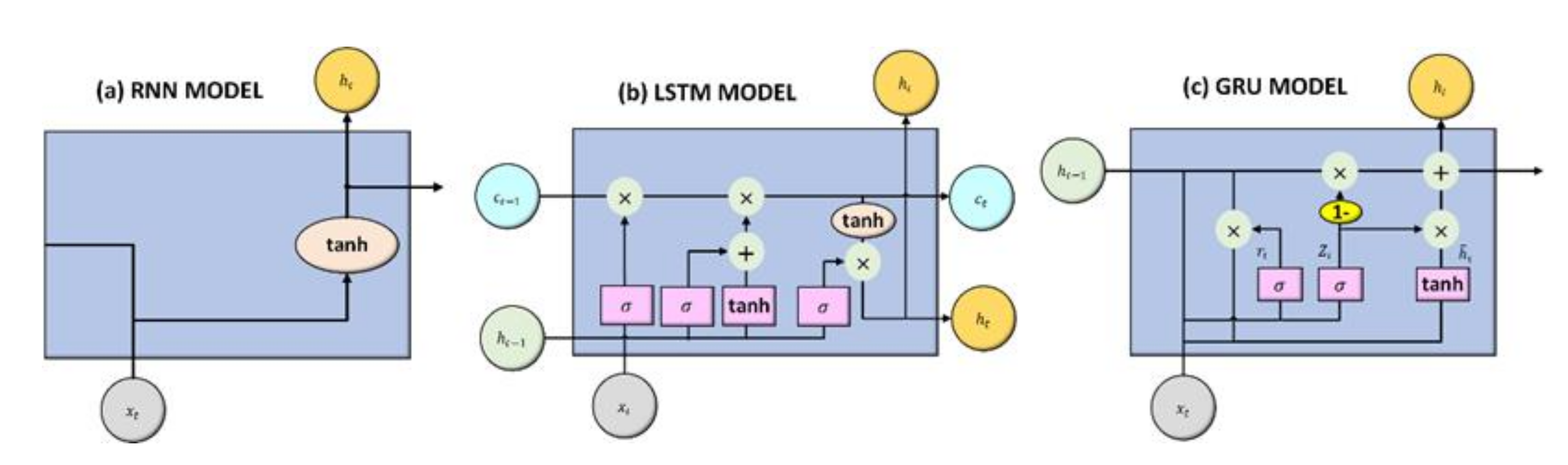
3.4. Time-Sequential Predictive Algorithm (RNN, LSTM, GRU, and Related Models)

The different time-sequential predictive models are utilized to validate and compare the capability and performance in predicting the generated solar power. In this study, the RNN, LSTM, and GRU are applied to explore efficiency and accuracy. In addition, the combination of bidirectional training with sequential predictive models is also utilized to evaluate the performance. The general structure of RNN, LSTM, and GRU is shown in Figure 1.

Recursive neural network (recursive neural network) is regarded as a generalization of the recurrent neural network, which is mainly based on the development of Rumelhart’s research results [49]. Its linear recursion on the time structure derive of the t vector will propagate to t-1, t-2, … Traditional RNNs can’t capture long-term memory because the final vector produces coefficients of continuous multiplication, resulting in the input of the starting vector in the forward process. The weak influence of the vector causes the problem of the disappearance of the gradient and causes the long-term memory to be hidden by the short-term memory. The RNNs that are designed to support sequences of arbitrary length can often only handle time sequences that are not too long [50].

The long short-term memory, which is a special type of RNN, has a significant advantage in consecutive events between relevant timestamps [51]. The LSTM has a lot of outperformed applications in renewable energy prediction [52,53]. The input, output, and forget gate in LSTM memory blocks could update and control the flow of consequent information which are relatively advantageous for the short-term prediction of renewable energy. The LSTM could continuously update the consequent data by utilizing the input, output, and forget gate of memory blocks.

In addition, Chung et al. proposed gated recurrent unit (GRU) which combines the input gate and forget gate in LSTM [54]. This lightweight version of LSTM could accelerate execution and reserve computational resources. The LSTM and GRU learning performance are significantly improved than traditional RNN when applied to different data sets and corresponding tasks.

In addition to the three models described above, the Bidirectional RNN was proposed by Mike Schuster in 1997 [55], which combined regular recurrent neural networks. The Bidirectional RNN extended the training process in the direction of positive and negative times. The results of the two training directions comprehensively state the transmission of recursive neural networks. The prediction value is generally performed in one direction from the front to the back, which can only be predicted through the previous information. The calculation process of the model may need to use the information from the future time. Therefore, the predictions could use the bidirectional to execute two one-way recursive neural networks at the same time and combine operations. The Bidirectional RNN provides the input value to these two recursive directions at the same time and the final output value is jointly determined by these two unidirectional recursive neural networks. In this study, the Bidirectional-simpleRNN, the Bidirectional-LSTM, and the Bidirectional-GRU are utilized to predict the generated solar power and the efficiency and accuracy are evaluated and compared.

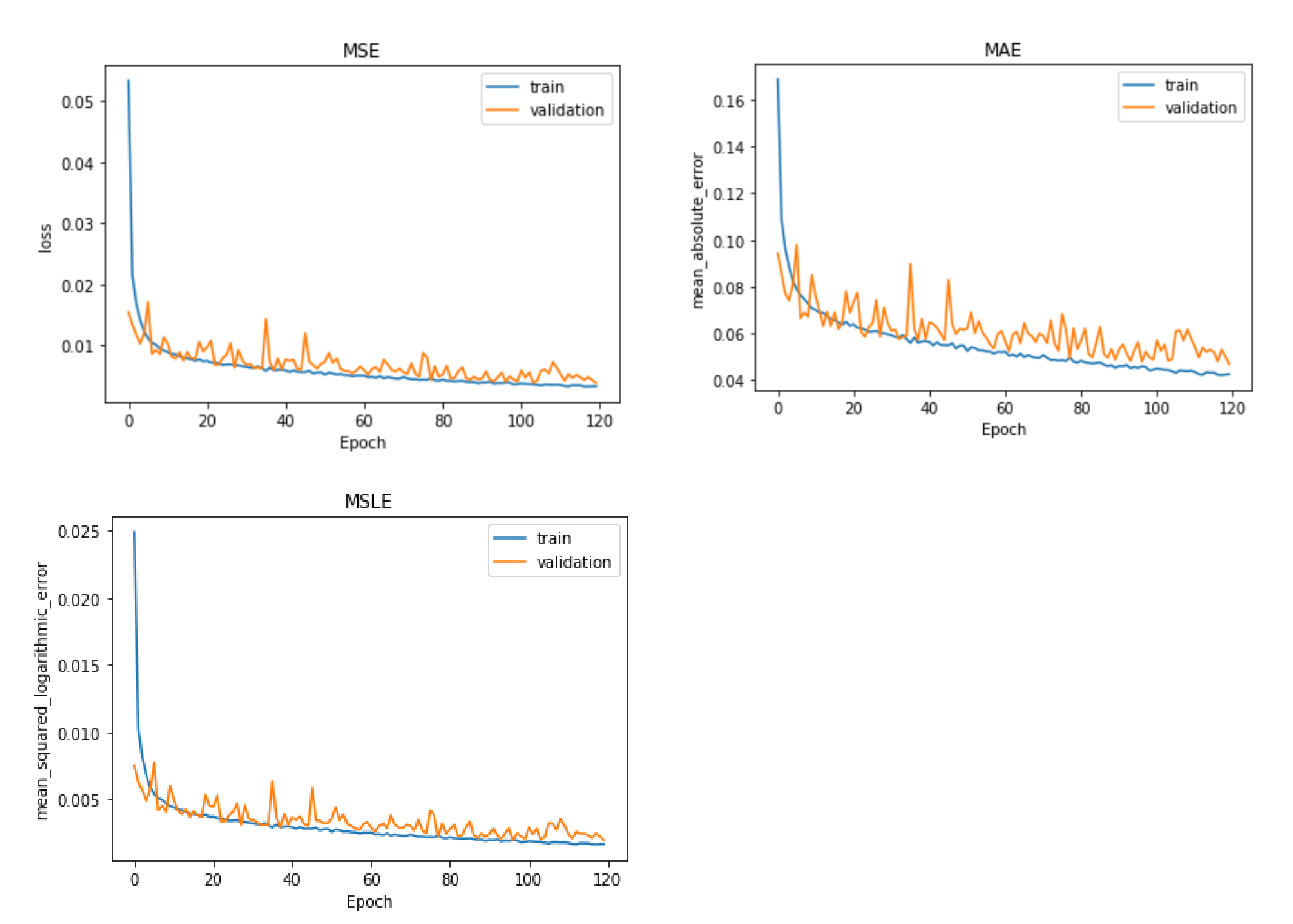
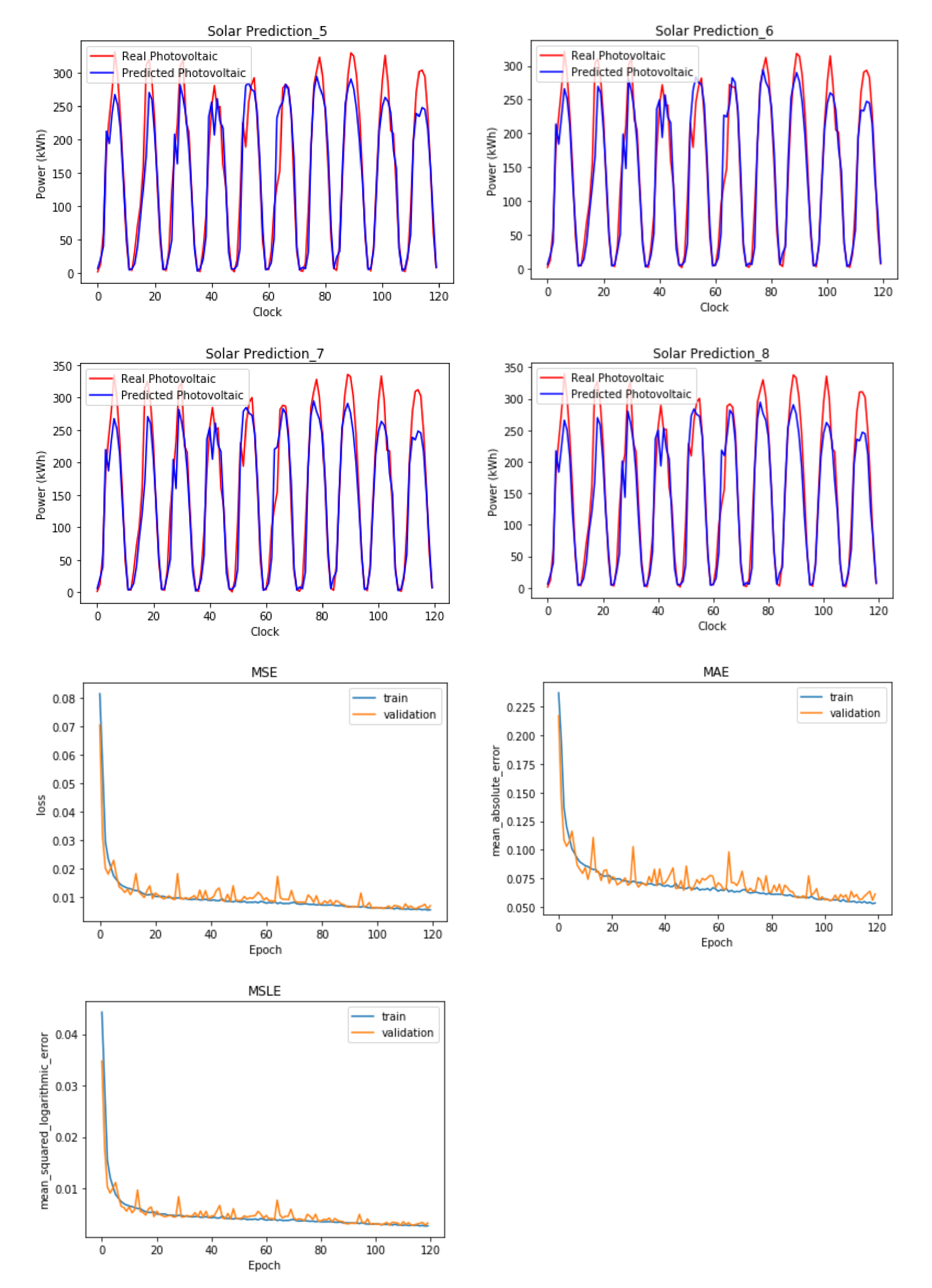
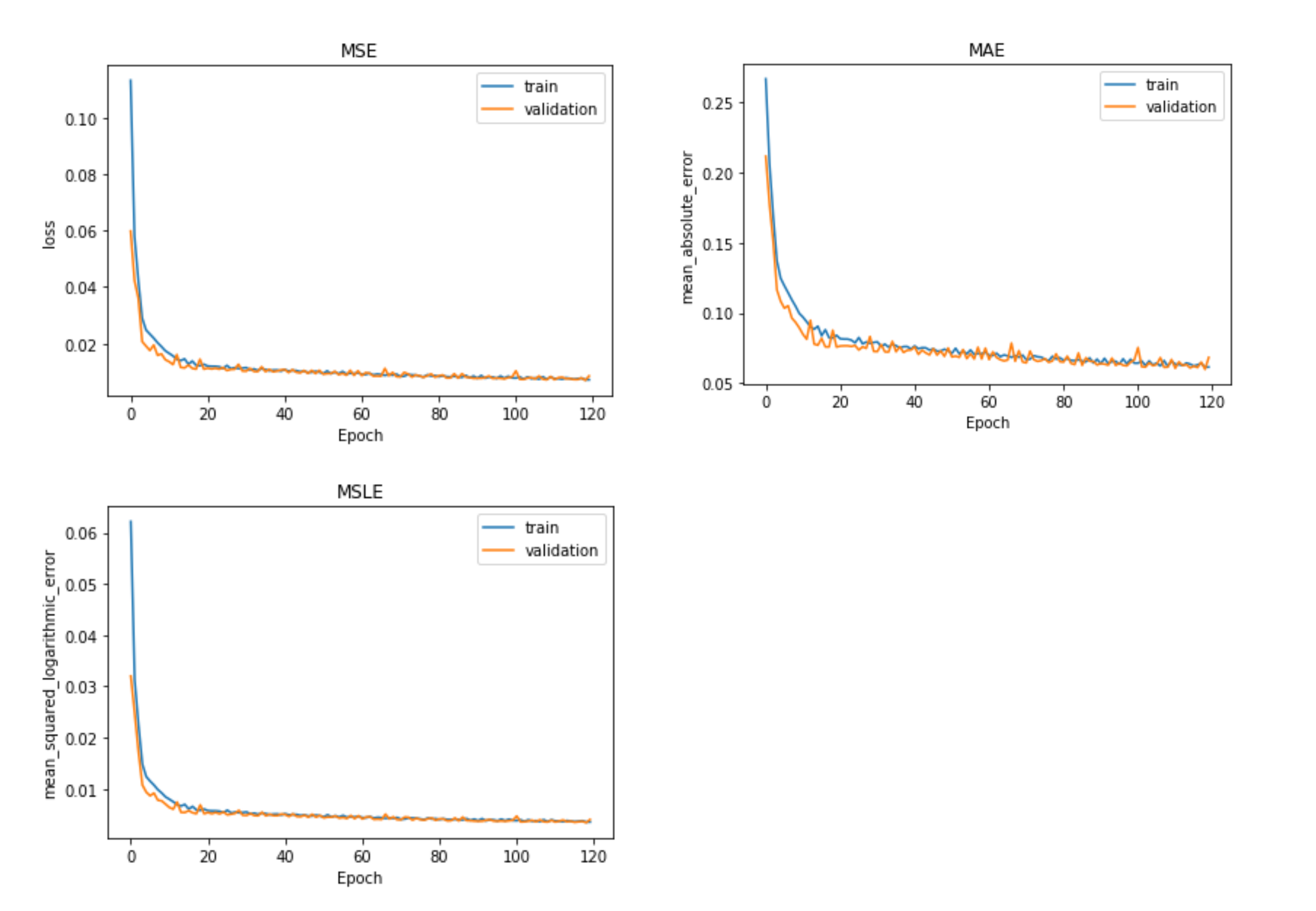
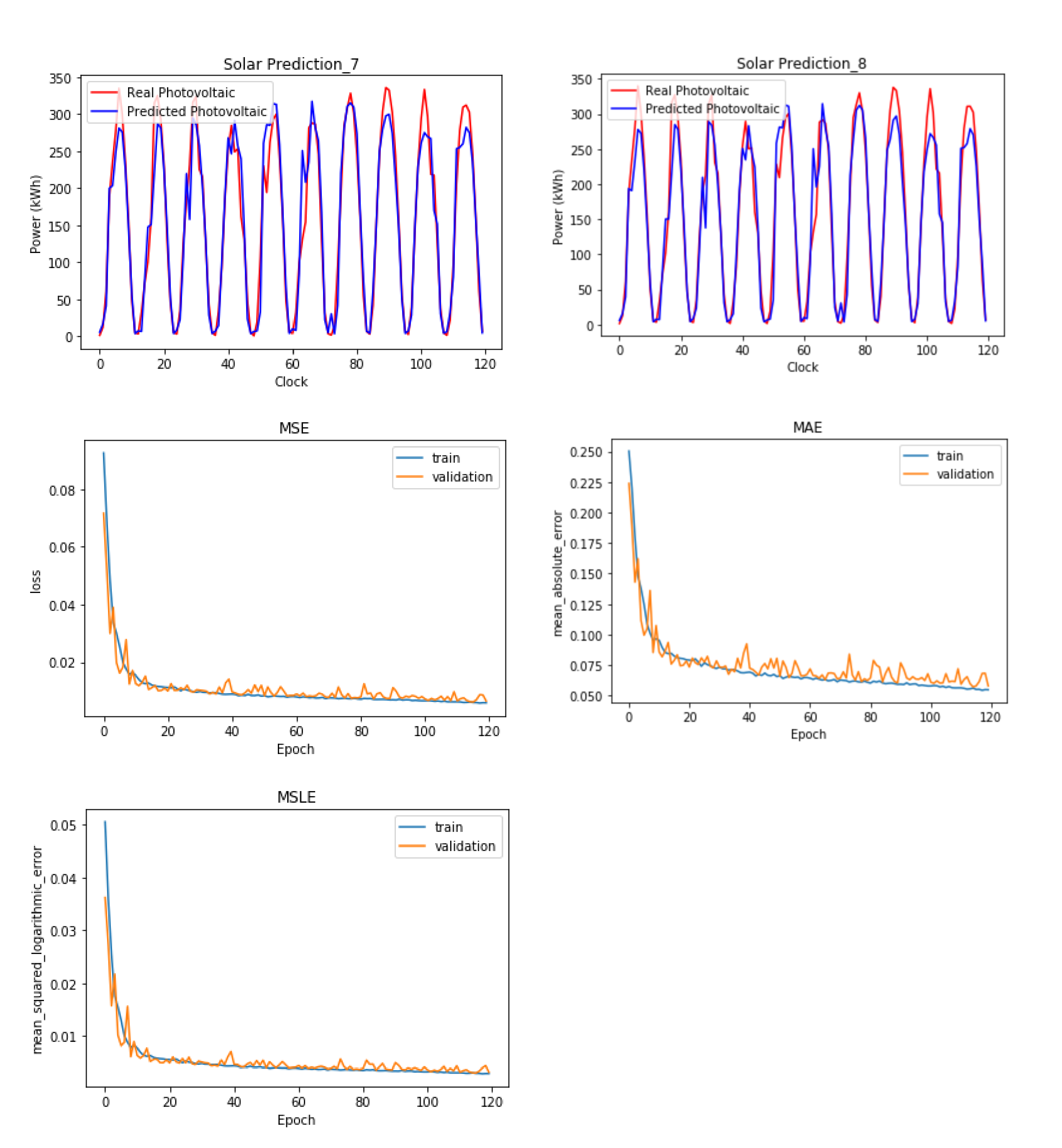
3.5. Predictive Model Parameters and Cross Validation

Most regression problems related to data used MSE to calculate the difference between the original and predicted values extracted by squared the average difference. We also use other functions likes MAE, which calculated the difference between the original and predicted values extracted by averaged the absolute difference, or the mean over the seen data of the squared differences between the log-transformed original and predicted values, it calls Mean squared logarithmic error (MSLE).

Therefore, it can be assumed that when n is the number of samples by the above calculation, $y_i$ is the actual value and $\widehat{y_i}$ is the predicted value. After compiling and calculating, we can get a performance indicator that is more than zero. When the value is more and more, it means the errors are more and more, which is defined as follows:

$$MAE=\frac{1}{n}{\displaystyle \sum }_{i=1}^n\left|y_{i-}{\widehat{y}}_i\right|$$

(3)

$$MSE=\frac{1}{n}{\displaystyle \sum }_{i=1}^n{\left(y_{i-}{\widehat{y}}_i\right)}^2$$

(4)

$$MSLE=\frac{1}{n}{\displaystyle \sum }_{i=1}^n{\left|\log \left(y_i+1\right)-\log \left({\widehat{y}}_i+1\right)\right|}^2$$

(5)

4. Experiments and Discussion

The main sources of research data used in this research are ambient air quality from the Environmental Protection Administration, weather-station observation data from Central Weather Bureau, and on-site monitoring system data of solar power plants. In the process of data collection, it has been discovered that the original data of the trilateral parties are stored and presented in different ways. So, the first step is converting the data into the array to stacking, and then merges all data according to the same timeline, and then through the artificial cross match. Finally, record the situation which is lost or unusual, and then the data will be eliminated and consolidated for a database.

At the beginning of this study, many difficulties were encountered in the collection of data. For example, the data fields were not completely, and multiple data sources were needed to compare with each other to fill in the missing fields. Due to the lack of fields, we tried many data sources, such as some government agencies and other data sources that provide real-time and historical climate inquiries. Although it seems that the completeness is relatively high, most of them are presented in a graphical way, which is slightly time-consuming in data conversion. In the data provided, only temperature and rainfall have clear values, and the rest must be found in other data sources or calculated manually. In this case, we have to find more data sources for data collection.

Therefore, this research data will use the historical data collected by the above trilateral parties from 7 November 2018 to 28 January 2020 (total 448 days) between 6 o’clock and 17 o’clock each day (total 12 h), it is used as the data of model of neural network. During the data collection period, the date when the abnormal data is found by manually checked is 39 days. Finally, the total data after the abnormal data is eliminated is 409 days.

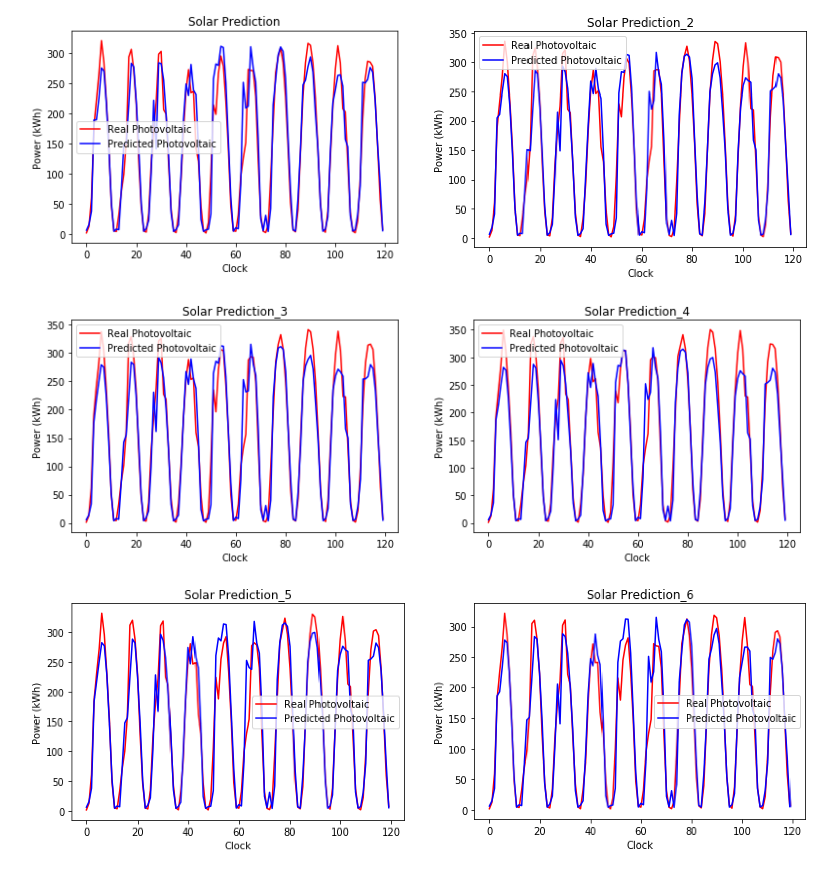
Finally, through the consolidated data, 80% of the early data (from 7 November 2018, to 31 October 2019, a total of 3948 records) recorded in the file are used as training data for the model to training, and the other 20% data (from 1 November 2019 to 28 January 2020, a total of 960 records) are used for testing, and then the testing data will be taken out for 10 days (1–10 January 2020, a total of 120 records) data is used as a visualization to present the forecast results.

Since this study is divided into two stages to execute multiple experimental schemes, in stage 1, it compares and descript model’s effect which used different feature variables; In stage 2, testing the influence of performance indicator which choose the different model. In this study, the above-mentioned experimental results uniformly use the coefficient of determination $r^2$ (R-Squared) as the evaluation standard of the performance indicator, and the value between [0,1] is obtained by the above-mentioned function calculation to determine the model fitting effect of is good or bad. Inside the function, the numerator is the summation of the difference of squares of original and predicted values, the denominator is the summation of the difference of squares of original and average values.

$$r^2=1-\frac{{{\displaystyle \sum }}_i{\left({\widehat{y}}_i-y_i\right)}^2}{{{\displaystyle \sum }}_i{\left({\overline{y}}_i-y_i\right)}^2}$$

(6)

4.1. Result of Feature Selection

Since the selection of feature variables will have the most obvious impact on the model prediction effect, the items with values less than ±1.0 after the analysis of feature variable correlation were eliminated at the beginning of the experiment, and the monitoring records on the site were used to implement the first experimental plan. Finally, using the performance indicator $r^2$ = 0.849865 of experimental program A-1. From this experiment, it can be found that the prediction effect by using the monitoring records on the site as the experimental sample is not good and still needs to be improved. Therefore, to make the performance of the model prediction more accurate, the subsequent experimental programs will be tried with different feature data samples. It is expected that the optimal results of the experiment can be obtained, then find the feature variables of the optimal model to extend subsequent research.

In the process of trying to improve the above experimental program. First, we combine the external meteorological with the on-site monitoring system information and obtain the effectiveness index $r^2$ = 0.853013 of the experimental program A-2 after training. When we compared it with the monitoring system that just referenced the on-site project, the features have been strengthened a lot. Secondly, the external environment is combined with the on-site monitoring system information and obtains the performance indicator $r^2$ = 0.860999 of the experimental program A-3 after training. Thirdly, above the external meteorological and environment is combined with the on-site monitoring system information and obtains the performance indicator $r^2$ = 0.865523 of the experimental program A-3 after training. Finally, it can be found that increasing the model’s feature category can effectively improve the model’s prediction situation by comparing the results of the above-mentioned experiments.

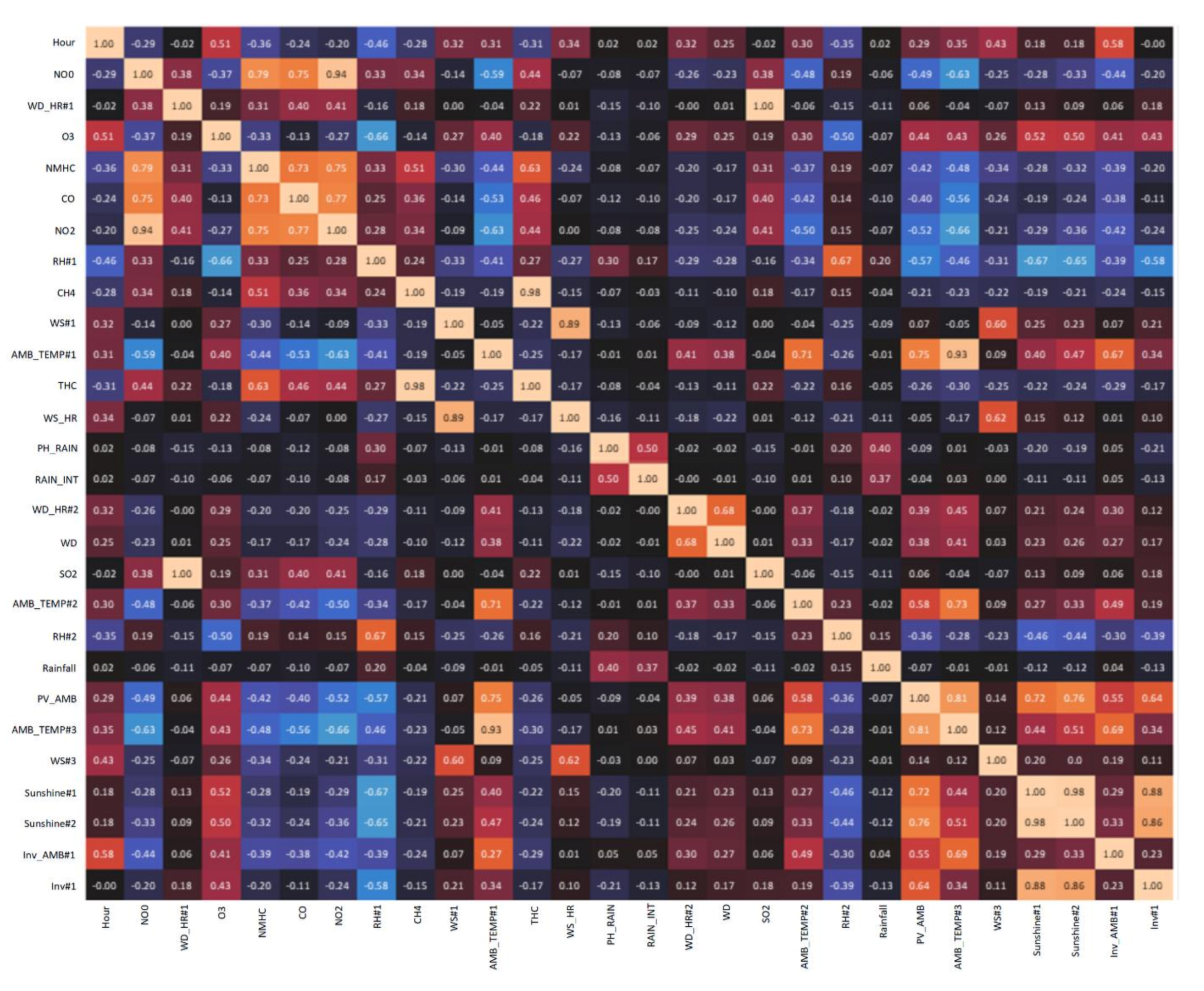
As the performance indicators of the experimental program, A-4 still have room for improvement, the results of the previous Pearson product-moment correlation coefficient analysis were used as the basis for screening, and the correlation coefficient was divided into 6 levels ± 0.2~0.3 according to the correlation coefficient. Figure 2 illustrates the resulting map of the Pearson correlation coefficient analysis. The list of feature variables of the data set used after Pearson correlation coefficient analysis is shown in

Table 3. List of feature variables of data set used after Pearson correlation coefficient analysis.

Source	Feature Variable
Environmental Protection Administration (Taiwan)	nitrogen oxide, hourly wind direction value, ozone, non-methane hydrocarbons, carbon monoxide, nitrogen dioxide, relative humidity, methane, wind speed, temperature, total hydrocarbons, hourly wind speed, acid rain, electrical conductivity, rainfall intensity, wind direction, sulfur dioxide.
Central Weather Bureau (Taiwan)	temperature, relative humidity, rainfall
Solar-power monitoring system information	inverter device temperature, solar cell module temperature, atmospheric temperature, wind speed, horizontal sunshine, module co-position angle sunshine

. According to the comparison of the results of the above 6 programs (A-5~A-10), when the experimental program A-5 is used to delete all the feature variables of the correlation coefficient +0.2~−0.2, the performance indicator $r^2$ = 0.880833 can be obtained, and the correlation of the feature variables is further compared. When the coefficient screening range is expanded to ±0.3, only the experimental program A-10 can obtain a better performance indicator $r^2$ = 0.845699 when all the feature variables of the correlation coefficient +0.3~0 are deleted. So, according to the above project of the results of the experiment, and finally the correlation coefficient +0.3~−0.2, feature variables are aggregated into the experimental program A-11, after training and prediction, the best performance indicator of the experiment at this stage is taken $r^2$ = 0.890179. There are 14 items of feature variables which are recording time, inverter device temperature, solar cell module temperature, atmospheric temperature, horizontal insolation, module corresponding angle insolation, relative humidity of external weather information, nitrogen oxides, ozone, non-methane hydrocarbons, nitrogen dioxide, relative humidity, temperature, and acid rain value of external environment information.

After the multiple experiment tests, it has been determined that A-11 is the optimized experimental result of this stage. Therefore, the remaining feature variables of the experiment were reviewed again. Some of the items were repetitive in nature, so the feature value item adopted in A-11 eliminates the relative humidity of the weather information and the temperature field of the environmental information in program A-11. Meanwhile, we implemented the linearly dependent experimental training with the prediction of experimental program A-12 and obtained the effectiveness index $r^2$ = 0.88494. However, in the end, it still failed to exceed the value of the effective index of program A-11.

Therefore, our experiment again tried to reassemble the equipment information data of the remaining 7 inverters on-site, external environment and information of weather, and on-site monitoring data into 8 training datasets. Besides, we take the best experimental program A-11 of this stage as the information sample of the stage 2 model experiment scheme, and try to obtain better solar power prediction result by changing the prediction model.

Finally, in stage 1, the results of the detailed performance indicator are presented in

Table 4. Pearson correlation coefficient comparison table.

Program	Evaluation Score (r2)
A-1	0.849865
A-2	0.853013
A-3	0.860999
A-4	0.865523
A-5	0.880833
A-6	0.876786
A-7	0.872881
A-8	0.835199
A-9	0.836241
A-10	0.845699
A-11	0.890179
A-12	0.884947

. The Stage 1 experimental summary of performance measurement indicators is shown in

Table 5. Summary of experimental performance measurement indicators (Stage 1).

Performance Measure	Score
mean_squared_error	0.010779
mean_absolute_error	0.076686
mean_squared_log_error	0.005071
${\mathrm{r}}^2$_score	0.890179

.

4.2. Experimental Results and Discussion

In this research process of experiment, besides the importance of aggregating strong correlative feature variables with generating solar power, the selection of prediction models is also to improve the performance. The most accurate and correlative feature variables are utilized to compare the effectiveness of different neural network models, which are the SimpleRNN, LSTM, GRU, Bi-SimpleRNN, Bi-LSTM, and Bi-GRU. The experimental program A-11 which has achieved the best performance measurement indicators, is utilized to demonstrate the effectiveness and accuracy during the training process. The originally configured in the initial stage between experimental models were identical, and the differences and changes were discussed. Stage 2 experimental summary of experimental performance using different models with measurement indicators among various programs is shown in

Table 6. Summary of experimental performance among different models with measurement indicators (Stage 2).

Experiment	Data Set with Different Models	$\mathbf{Score}\left({\mathit{r}}^2\right)$
B-1	Data set A-11 with LSTM model	0.914729
B-2	Data set A-11 with GRU model	0.859122
B-3	Data set A-11 with SimpleRNN model	0.733053
B-4	Data set A-11 with Bidirectional-LSTM model	0.904538
B-5	Data set A-11 with Bidirectional-GRU model	0.934156
B-6	Data set A-11 with Bidirectional-SimpleRNN model	0.765555

.

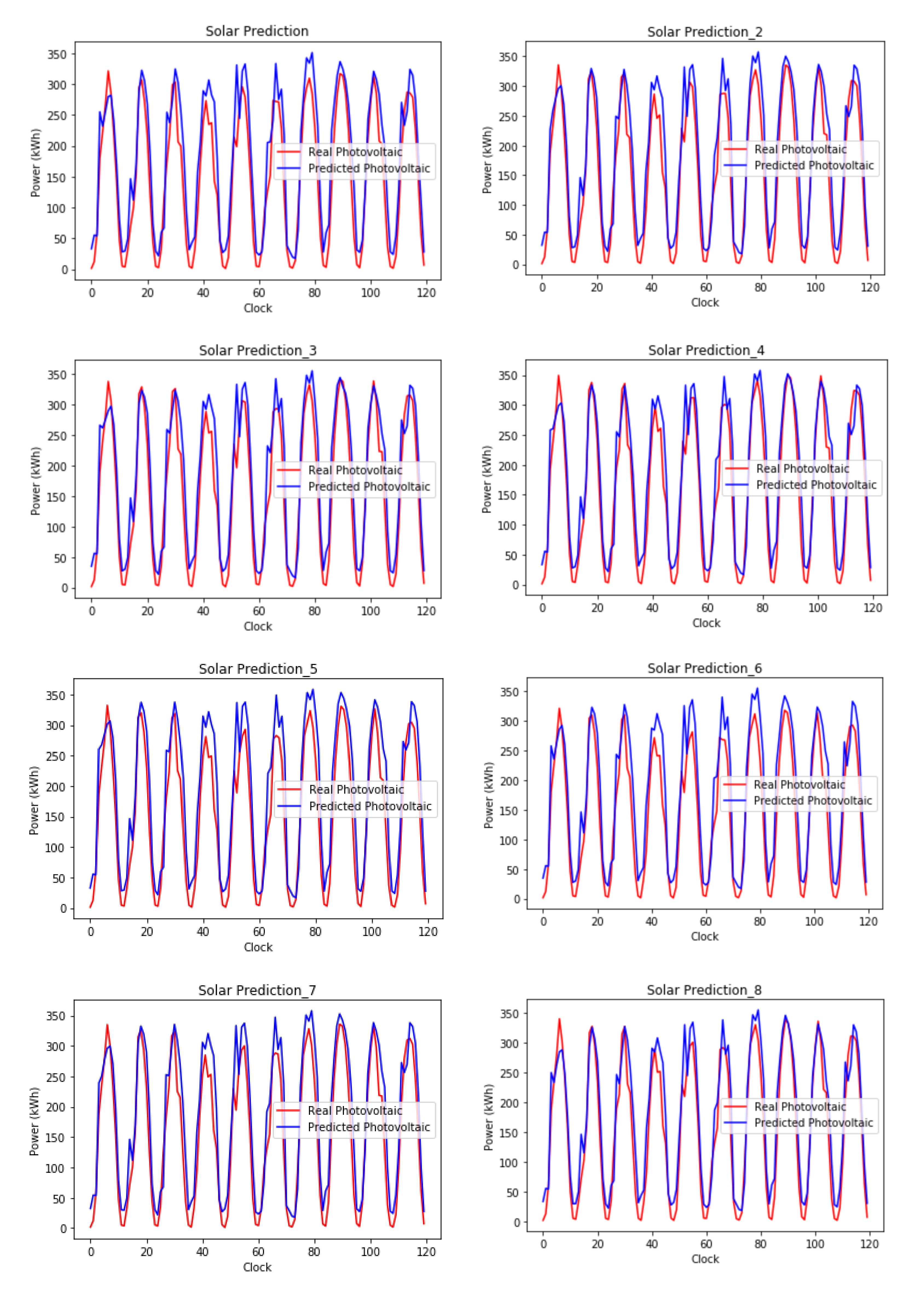
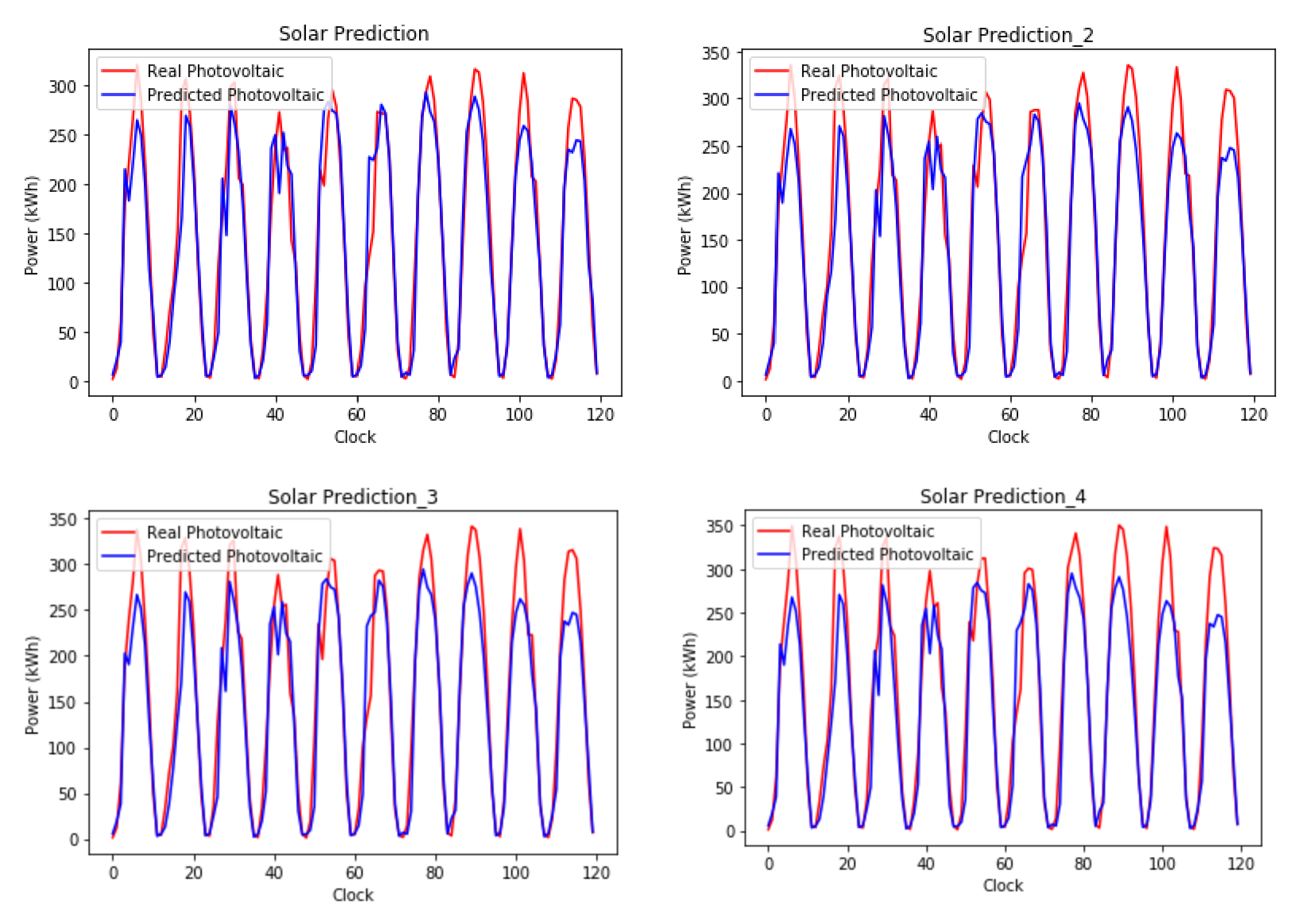
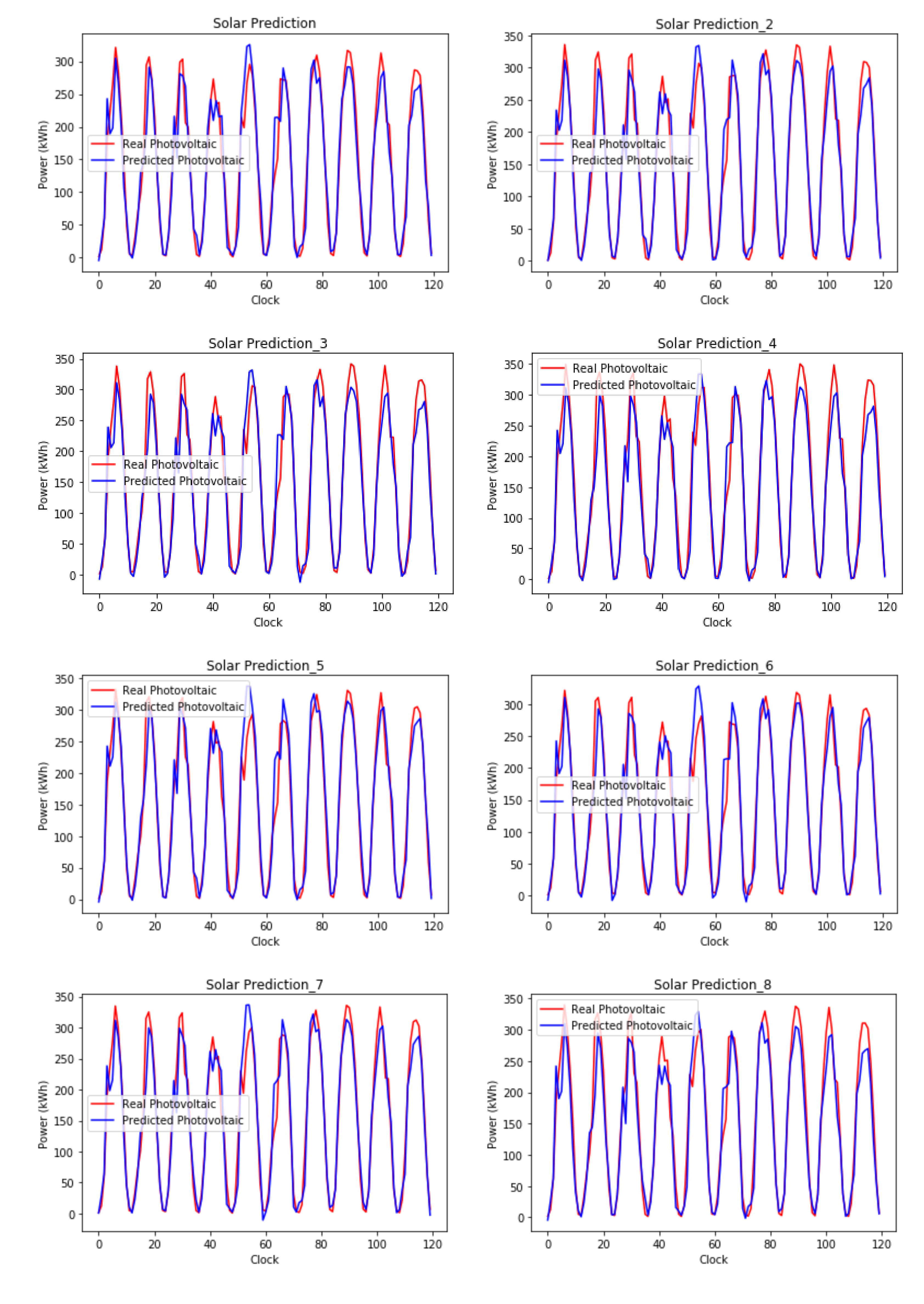
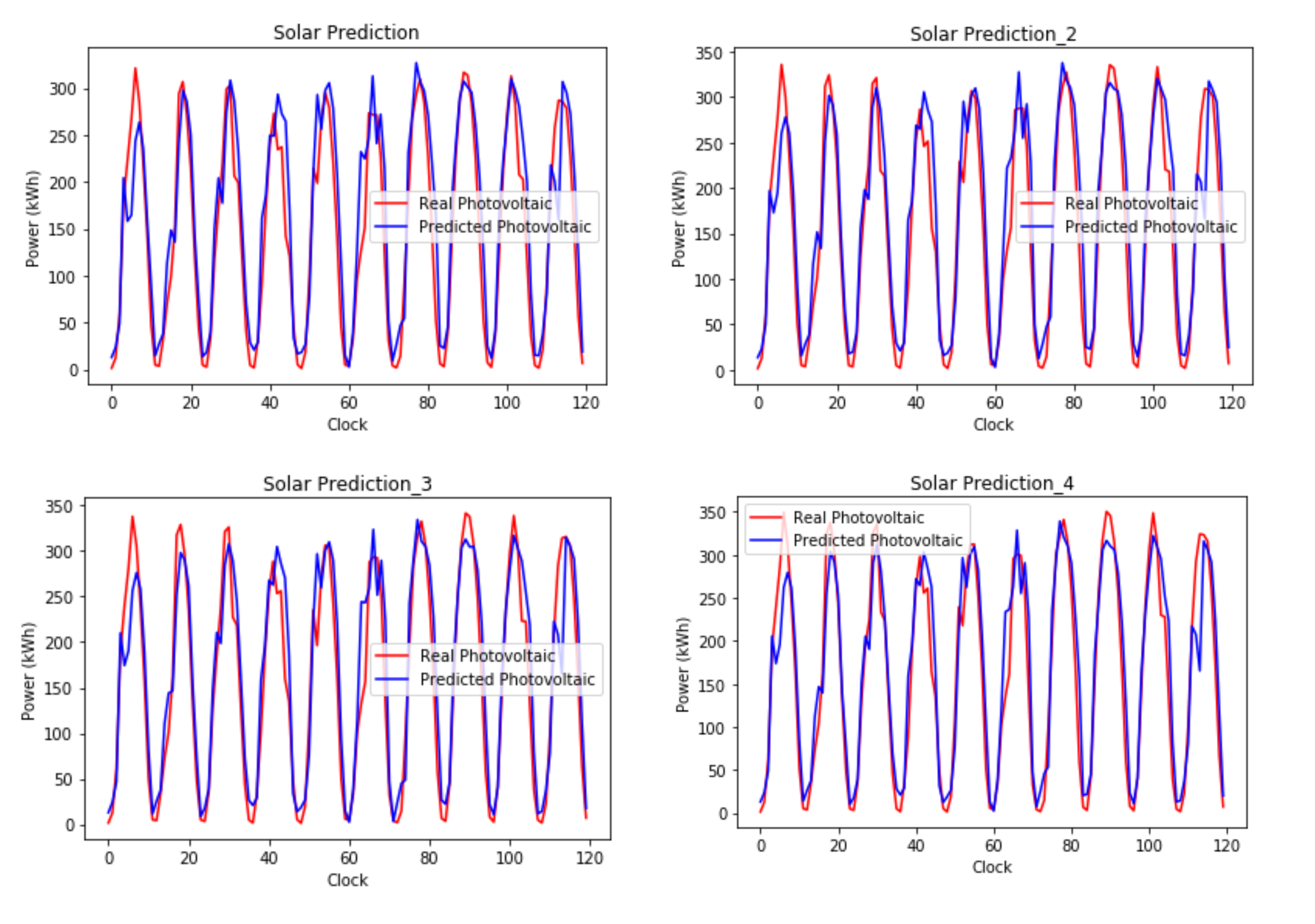
Firstly the neural network models were executed separately several times, which selected the best performance experimental results for discussion. The training process and solar generation prediction in different sceneries are shown in Figure 3, Figure 4, Figure 5, Figure 6, Figure 7 and Figure 8.

From Table 5, the SimpleRNN, which is essentially the most intuitive and most basic regression model, has less performance comparing with the improved LSTM and GRU. In addition, although the GRU is an improved version of LSTM and the training time required for GRU is indeed slightly reduced, the performance of GRU predictions generally cannot be equal to or exceed the performance of LSTM. Therefore, by exploring the conclusions of the differences in the effectiveness of the above three algorithms, the SimpleRNN is recommended for basic simple calculations. Secondly, if the experimental development process needs to deal with a huge data set in order to obtain preliminary experimental evaluation results, the application of GRU will be the first choice. However, if an accurate in depth calculation prediction model is required, the LSTM model is recommended as the main execution algorithm. Although the execution process requires high system resources and training time, the overall situation is relatively stable, reliable, and accurate. Since the above three models are all one-way training methods, the final verification method was used the bidirectional packaging model to attempt the optimal results through the two-way transmission of the model training process. According to Table 5, when the bidirectional -LSTM model is utilized, although the bidirectional-LSTM model can indeed reduce the difference in each training result, the R square value showed no better performance. Furthermore, when the Bidirection-SimpleRNN model is also used as the experimental scheme, the bidirectional packaged model can effectively improve the gradient descent of the training process. However, the prediction effect of the Bidirection-SimpleRNN model itself is not good, resulting in poor final results. Ideally; when the GRU model is finally used as the bidirectional packaging, this bi-direction model has increased the difference in the effectiveness of the training results. The bi-direction ability has allowed the GRU model has streamlined the calculation method of the LSTM model and achieve better performance, and finally achieved the optimized performance index of this research, as R square equals 0.934156, in the experimental program B-5.

5. Conclusions

The main purpose of this research is to explore the prediction and evaluation methods of solar power generation. Therefore, in this work, we conducted intensive experiments using deep learning models to effectively predict power generation from our experimental results. It has been confirmed through the prediction of experiment A-1, that only using the monitoring system data on-site installed in the solar power plant cannot effectively establish an accurate prediction model. The actual applications still need to collect other possibly related feature data, and it may make the solar power prediction model gradually improved to optimization through different model experiments.

Since it only uses the related feature values and the data set of a single inverter which are collected in the above experiment (total 3948 training data) for training, the performance indicator predicted by the model can only be increased to $r^2$ = 0.890179. So once again, the concept of a Generative adversarial network (GAN) is extended to multiple inverters (8 sets of training data total 31584), then aggregated and reshaped the dataset by the temperature of the inverter and the feature variables. Finally, experiment B-5 obtains the optimal performance indicator of $r^2$ = 0.934156 by using the Bidirectional-GRU model. These feature variables used in the optimal prediction results will increase the prediction effect of power generation. The most likely reason is the correlation between the greenhouse effect and solar thermal radiation. Therefore, if it is necessary to further strengthen the prediction accuracy in the future, it is recommended to collect the relevant feature variables of the solar irradiance or the greenhouse to obtain better results. Currently, there are many new and improved neural networks that can be applied to the study. In future work, the methods using a hybrid deep learning model can be considered into the system to continuously improve the prediction performance of solar power generation.