Dynamic Aeroelastic Response of Stall-Controlled Wind Turbine Rotors in Turbulent Wind Conditions

Abstract

With the current global trend of the wind turbines to be commissioned, the next generation of state-of-the-art turbines will have a generating capacity of 20 MW with rotor diameters of 250 m or larger. This systematic increase in rotor size is prompted by economies-of-scale factors, thereby resulting in a continuously decreasing cost per kWh generated. However, such large rotors have larger masses associated with them and necessitate studies in order to better understand their dynamics. The present work regarding the aeroelastic behavior of stall-controlled rotors involves the study of the frequency content and time evolution of their oscillatory behavior. A wide range of experiments were conducted to assess the effects of rapid variations on the rotor’s operational conditions. Various gust conditions were tested at different wind speeds, which are represented by pulses of different intensities, occurring suddenly in an otherwise constant wind regime. This allowed us to observe the pure aero-elasto-inertial dynamics of the rotor’s response. A reduced-order characterization of the rotor’s dynamics as an oscillatory system was obtained on the basis of energy-transfer principles. This is of fundamental interest for researchers and engineers working on developing optimized control strategies for wind turbines. It allows for the critical elements of the rotor’s dynamic behavior to be described as a reduced-order model that can be solved in real time, an essential requirement for determining predictive control actions.

1. Introduction

Renewable energy production, especially wind power, has been growing over time to become an important source for providing for electricity and fuel demands. Technological advances have made wind the fastest-growing renewable energy technology in electricity generation systems. Following the current global trend of the wind turbines to be commissioned and the studies conducted by the European Wind Energy Association (EWEA), the next generation of state-of-the-art turbines will have a generating capacity of 20 MW with rotor diameters of 250 m or larger [1]. This systematic increase in rotor size is prompted by economies-of-scale factors, thereby resulting in a continuously decreasing cost per kWh generated. However, such large rotors have larger masses associated with them and necessitate studies in order to better understand their dynamics. This has led to numerous efforts on the development of suitable control approaches [2,3,4,5]. Bianchi et al. [6] provided details on some common load control methodologies. Among the ones that have been studied and implemented in the context of utility-scale wind turbines are stall control [7], pitch control [8], active stall control [9], and passive control using aeroelastic devices [10].

In all cases, wind turbine control systems have to deal with the challenges of an intermittent and difficult-to-predict source of energy. Wind, by its very nature, varies with place and time, making energy conversion difficult. This calls for the development of improved technologies that efficiently harness energy from the available wind resources, and advanced control systems are a key research aspect of wind turbine technology [11]. Such systems are needed to maximize the output power at low wind speeds, limit rotor power at wind speeds above the nominal value, and reduce fluctuating loads on the turbine blades that may compromise their long-term operational life [12]. That is, the basic objective is to maximize the rotor’s power production for wind speeds below the nominal level and limit it for wind speeds above the nominal level, keeping it as close as possible to the nominal power of the drive train in order to avoid exceeding the nominal power of the shafts, bearings, gear box, generators, and power electronics.

Among the several families of control methods mentioned above, pitch and stall control have been by far the most commonly used in modern utility-scale machines. Both are based on altering the aerodynamic characteristics of the blade sections in order to control the forces that produce the rotor’s torque, power, thrust, and deformation. By rotating the blades around their root, pitch-control systems allow us to smoothly change the aerodynamic forces acting on the blade by altering the angle of attack on the airfoil blade sections. By changing the tangential projection of the aerodynamic force (which is the one contributing to the driving torque), pitch systems can smoothly control the rotor’s output power. In stall-control turbines, the blades are rigidly attached to the hub. Thus, the setting angle of every airfoil section along the blade span is fixed.

In the classic fixed-speed stall-control method, the rotational speed of the rotor is kept constant at its nominal value, and the geometry of the blades is designed in such a way that, as the wind speed increases above the nominal value, the angle of attack of the flow incoming onto the blade’s airfoil sections increases, and a larger portion of the blade span enters into stall. The stall condition is characterized by the separation of the boundary layer on the rear-upper surface of an airfoil section at high angles of attack. Separation disrupts the flow circulation and alters the pressure distribution, drastically reducing lift and increasing drag. The overall result is that the portions of the blade span that enter into stall stop contributing to the driving torque, limiting the rotor’s power production. The stall transition is not intended to occur simultaneously all over the span. The method works by gradually changing the portions of the blade span that are in the stall or attached regime. Stall starts at the inner portions of the blade and close to the root, and then progresses towards the tip.

With the stall method, the elimination of the pitch mechanism lowers the capital cost and reduces maintenance expenses. The elimination of the pitching mechanism is particularly important when considering the systematic increase in turbine size that has been taking place over the last 30 years. This process, sometimes referred to as upscaling, is prompted by economies of scale, which reduce the cost of energy production, and this is likely to continue in the future. One of the consequences of upscaling is the substantial increase in the blade mass per unit energy produced, as the blade mass depends on the cube of the rotor’s diameter, while the energy captured depends on the rotor’s swept area (i.e., the diameter’s square). In addition to the aspect of the construction and material costs, this so-called "square–cube law" implies that the size and cost of the pitching mechanisms (and the energy required for their actuation) would increase much faster than the increase in the energy produced as the turbine size increases. Thus, the elimination of the pitch mechanisms by adopting some form of stall control would represent a big advantage for the next generation of high-capacity wind turbines with much larger blades [13].

Our current research consists of the investigation of the aeroelastic behavior of a stall-controlled rotor by involving the study of the frequency content and time evolution of the oscillatory behavior in order to gain a better understanding of the underlying physics. To this end, we conducted a wide range of experiments to assess the effects of rapid variations on the rotor’s operational conditions, such as gusts and turbulent fluctuations in the wind flow. To systematize this analysis, various gust conditions were tested for different wind speeds. These were represented by pulses of different intensity, occurring suddenly in an otherwise constant wind regime. This allowed us to observe the pure aero-elasto-inertial dynamics of the rotor’s response. We then focused on obtaining a reduced-order characterization of the rotor’s dynamics as an oscillatory system based on energy-transfer principles. In addition to its intrinsic scientific value, this aspect of the work presented here is of fundamental interest for researchers and engineers working on developing optimized control strategies for wind turbines. It allows for the critical elements of a rotor’s dynamic behavior to be described as a reduced-order model that can be solved in real time, an essential requirement for determining predictive control actions.

2. The Numerical Model

In this section, we shall provide a brief description of a novel member of the BEM model family used in our research, which is called the Dynamic Rotor Deformation–Blade Element Momentum model (DRD-BEM) and was introduced in Ponta et al. [14]. This model accounts for the aerodynamic effects of the misalignments at every blade section. This is achieved by transforming the velocity and force vectors across different coordinate systems—from the coordinate system of the free-stream wind to the coordinate system of the blade section. These coordinate transformations are performed with a set of orthogonal matrices that account for all forms of misalignments at each instance. These include misalignments brought about by blade deformation, mechanical inputs such as pitching and yawing, or even pre-conformed misalignments, such as pre-bending of the original blade.

The DRD-BEM is coupled with an advanced technique used to simulate the structural response of the blade that is based on the Generalized Timoshenko Beam Model (GTBM). The GTBM, a dimensional reduction method, has the same parameters as the traditional Timoshenko model and can work for complex beams that may have twisted or curved shapes. In this model, originally introduced by Prof. Hodges [15,16], the beam section does not remain planar after deformation, and a 2-D finite element mesh is used to interpolate the warping of the deformed section. A mathematical formulation is then used to write the 3-D strain energy in terms of the classical variables of the 1-D Timoshenko model. The complexities of the 3-D model and geometry of the blades are reduced into a stiffness matrix for the corresponding 1-D beam. This 1-D beam can then be solved along a reference line representing the beam’s axis on the original configuration, and it can curve in any direction after deformation. A new coordinate system is introduced to represent the dynamic and kinematic variables along the reference line. This system follows the blade deformation into the instantaneous configuration. The blade sections in the chord-normal, chord-wise, and span-wise directions stay aligned with the intrinsic system. Therefore, accurate position tracking can be achieved by using this technique, even in cases of large displacements or rotations of the blade section. The GTBM technique uses a fully populated $6\times 6$ stiffness matrix instead of only six stiffness coefficients, as in the classical Timoshenko theory, which gives it the capacity to represent the effects of coupled modes of deformation, such as bend–twist. More details about our implementation of the GTBM and its coupling with DRD-BEM can be found in Otero and Ponta [17] and Ponta et al. [14].

The inertia properties are also dimensionally reduced to produce a $6\times 6$ inertia matrix for the equivalent beam along the reference line L. This inertia matrix contains the moments of inertia of both first and second order for blade sections along the span. These are acquired from a 2-D integration that operates over the area of each blade section and also considers the distribution of material properties and the details of the blade section’s shape. These matrices operate on the linear and angular velocities, which give the linear and angular momentum of the vibrational motion, as well as the inertia forces and moments associated with them. We can also calculate the inertia forces of the rotation of the main shaft and of mechanisms such as pitch and yaw. Therefore, all parameters, such as the angular, linear, centrifugal, and acceleration effects, are taken into account in a full 3-D representation.

The aforementioned interaction of structural and aerodynamic modules can maximize the capabilities of this advanced model. The equations of motion of the equivalent beam modeled as a 1-D finite element problem are solved by means of a non-linear adaptive ODE algorithm. Moreover, the ODE algorithm used to integrate the structural and aerodynamics module can easily be extended to include other modules in order to simulate the response of control systems, electro-mechanical devices, etc. This type of solver checks the solution by tracking the truncation error at each time step. The control system can be modeled by adding differential equations to the general ODE algorithm. This nonlinear adaptive ODE algorithm, which is used as a “common framework”, can be extremely useful as a way to integrate the solutions of all multi-physics aspects of the problem. A flowchart of the scheme demonstrating the interaction between the different modules can be seen in Ponta et al. [14]. This modular design of a multi-physics model, which is called the Common ODE Framework (CODEF), can help to simplify code development by independently improving each sub-model. Therefore, analyses of the aeroelastic problem and innovative control strategies that include mechanical and electrical aspects can be performed simultaneously by using an integral and computationally efficient solution through a self-adaptive algorithm.

A detailed description of the implementation of the DRD-BEM model can be found in Ponta et al. [14] and the references therein. Menon and Ponta [18] reported results of the application of the DRD-BEM to the analysis of the aeroelastic dynamics of rotors undergoing rapid pitch-control actions, and Otero and Ponta [19] used the model to analyze the effects of blade section misalignment on cyclic loads on a rotor. Ponta et al. [14] and Otero and Ponta [17] presented the details of the structural model. Additionally, Ponta et al. [14] also included results of the DRD-BEM model when applied to the analysis of vibrational modes of composite laminated wind turbine blades together with validation results against the works of Jonkman et al. [20] and Xudong et al. [21].

3. Reduced-Order Characterization of the Aero-Structural Interaction

3.1. Objectives and Methodology

Following a limited set of preliminary experiments reported in Jalal et al. [22], we conducted an extensive series of experiments on the aero-elasto-inertial response of wind turbine rotors by using Delft University’s stall-control rotor (see Jaimes [23]), an alternative to the NREL-5MW-RWT benchmark turbine. The DU-5MW stall RWT has a nominal wind speed of 15.3 m/s and a nominal rotational speed of 10.7 rpm. By studying the time evolution of the rotor’s oscillatory behavior when stimulated by pulses in the wind of controlled amplitude and time span (see Figure 1), we gained a deeper understanding of the underlying physics. We also obtained a reduced-order characterization of the rotor as an oscillatory system based on the principle of energy transfer between the kinetic energy of the wind-speed pulse and the elasto-inertial energy accumulated in the rotor. These wind pulses are mounted on top of a uniform stream inflow of different constant speeds covering the entire operational regime of the turbine from 5 to 25 m/s. The resultant study provides extremely valuable information to the wind power control community in order to produce Reduced-Order Models (ROMs) that could be solved in real time to develop predictive control strategies.

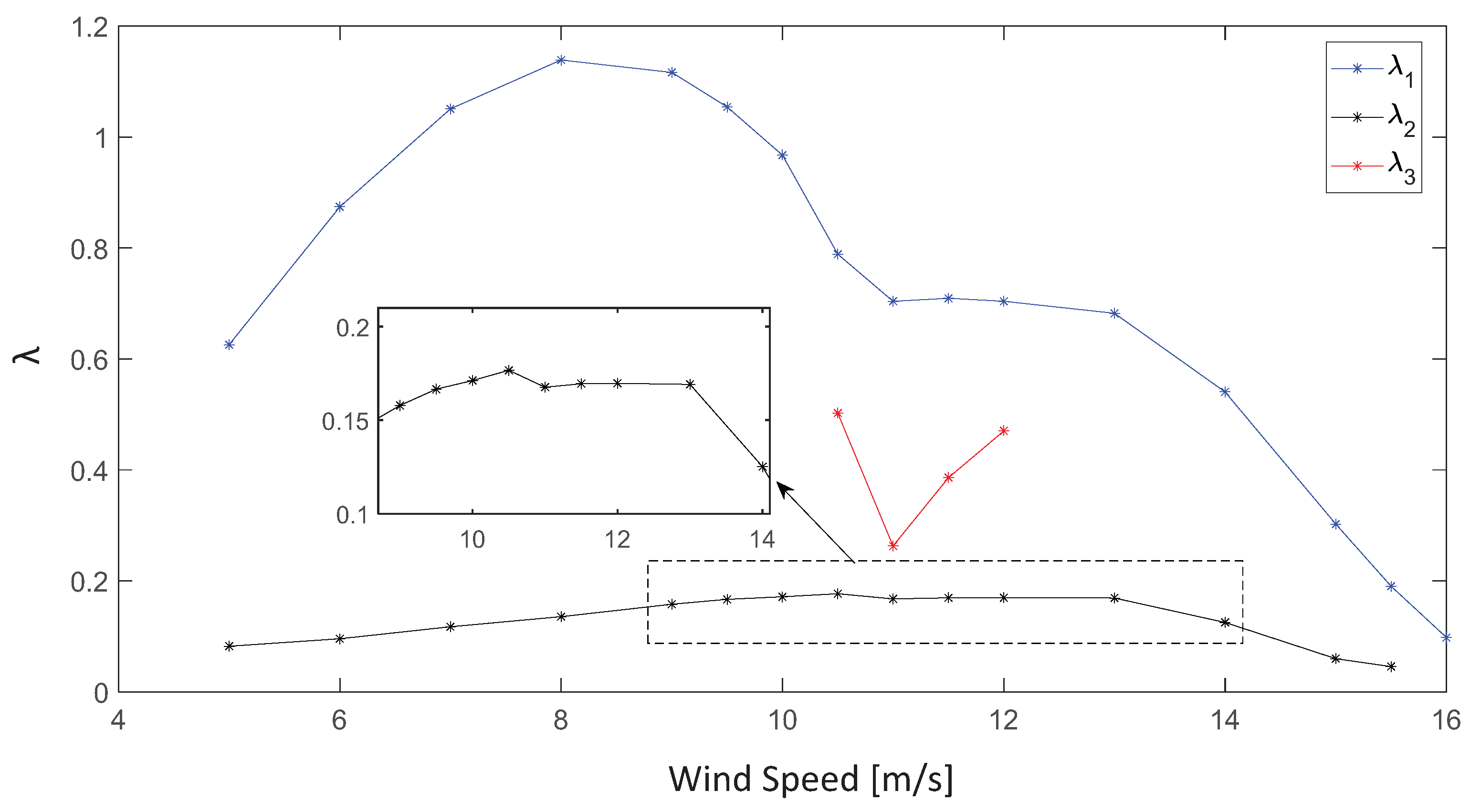
3.2. Wind-Speed Stability Threshold and the Role of Aerodynamic Damping

For wind speeds between 5–16.5 m/s, we found that the dynamic oscillatory response of the rotor remains stable. The kinetic energy of the wind pulse initiates oscillations, and those oscillations become damped by the system, creating a decay in the oscillatory signal (which is observable in the time evolution of the axial component of the blade deflection depicted in Figure 2 and Figure 3). Here, $U_{hx}$ represents the instantaneous axial deflection of the blade about its equilibrium value corresponding to the deformation state induced by a certain constant $W_{\infty }$.

Above 17 m/s, the rotor, as an oscillatory system, no longer damps the oscillations, but amplifies them, feeding on the energy from the wind flow. After the pulse has passed, the oscillations continue expanding exponentially until a second damping mechanism starts to act, slowing the growth and reaching an equilibrium where the oscillation amplitude becomes stable and self-sustained.

As we will see in detail in the following, this change in behavior from stable to unstable oscillatory regimes is associated with a change in sign of the aerodynamic damping. This depends exclusively on the mean value of the wind speed.

Between the stable and unstable regimes, there is a narrow range of wind speeds that exhibit the classical signs of a transitional behavior where attenuation and amplification may occur. Here, we see two examples (even though several variations are possible).

For wind speeds that are early on in the transitional regime (Figure 3a), the system starts damping the oscillations, but they are not completely dissipated, and some residual “bands” of oscillation remain. Further, at higher wind speeds in this regime (Figure 3b), expansion occurs, followed by a brief stabilization, and then the oscillations decay. The same manifestation of sustained residual oscillations is present in the long term.

This regime is characterized by a very rich combination of frequencies whose amplitudes evolve in time in a very complex manner.

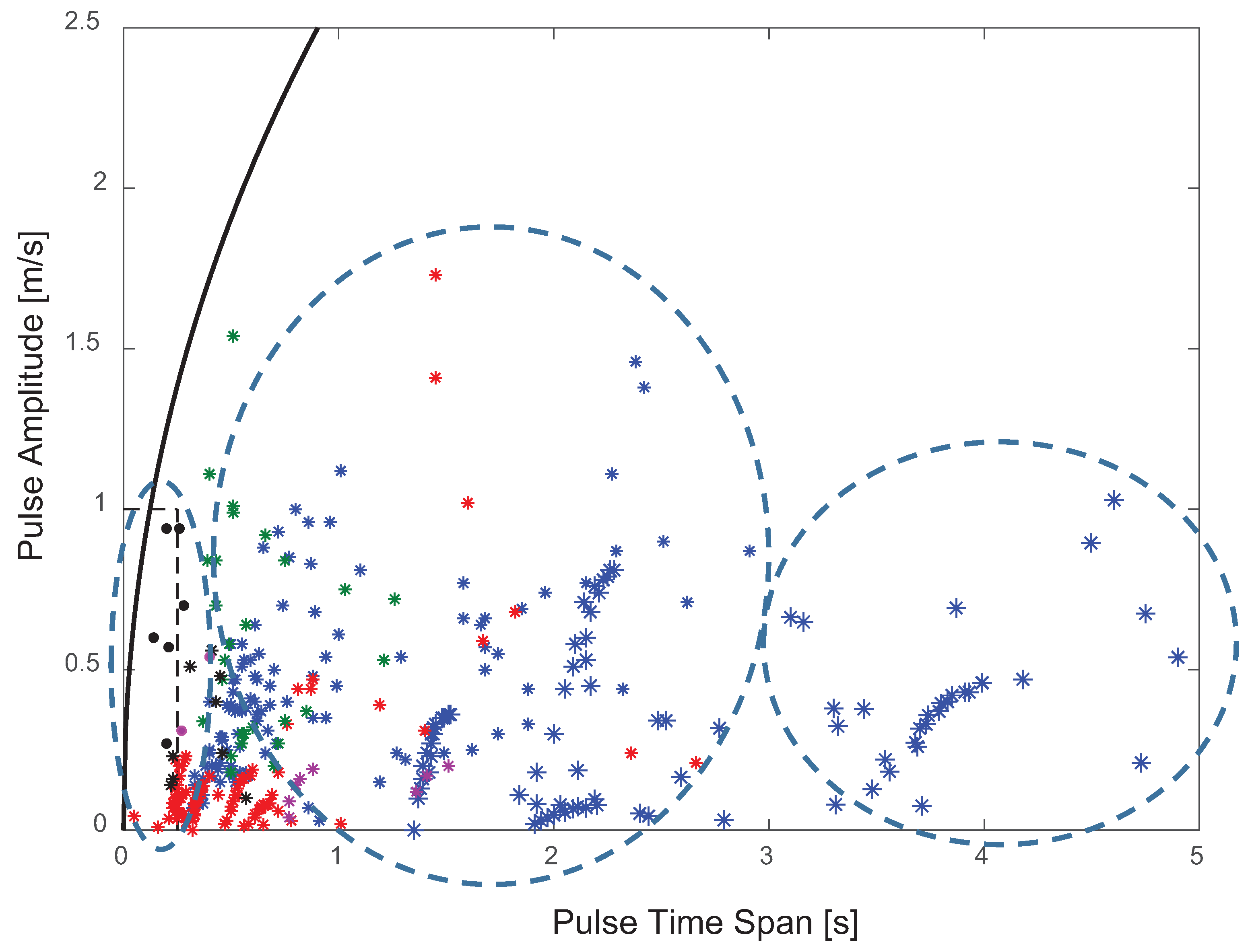
3.3. Characterization of Pulses Representing Typical Atmospheric Flow Oscillations

Our objective was to identify and quantify pulses with a characteristic time span and amplitude that represent typical oscillations in wind speed in a statistical sense. We collected samples of anemometry data from different sources and classified them in an amplitude versus characteristic time span chart (see Figure 4). We found three distinguishable regions in this chart, which are indicated by encircling elliptical dashed lines.

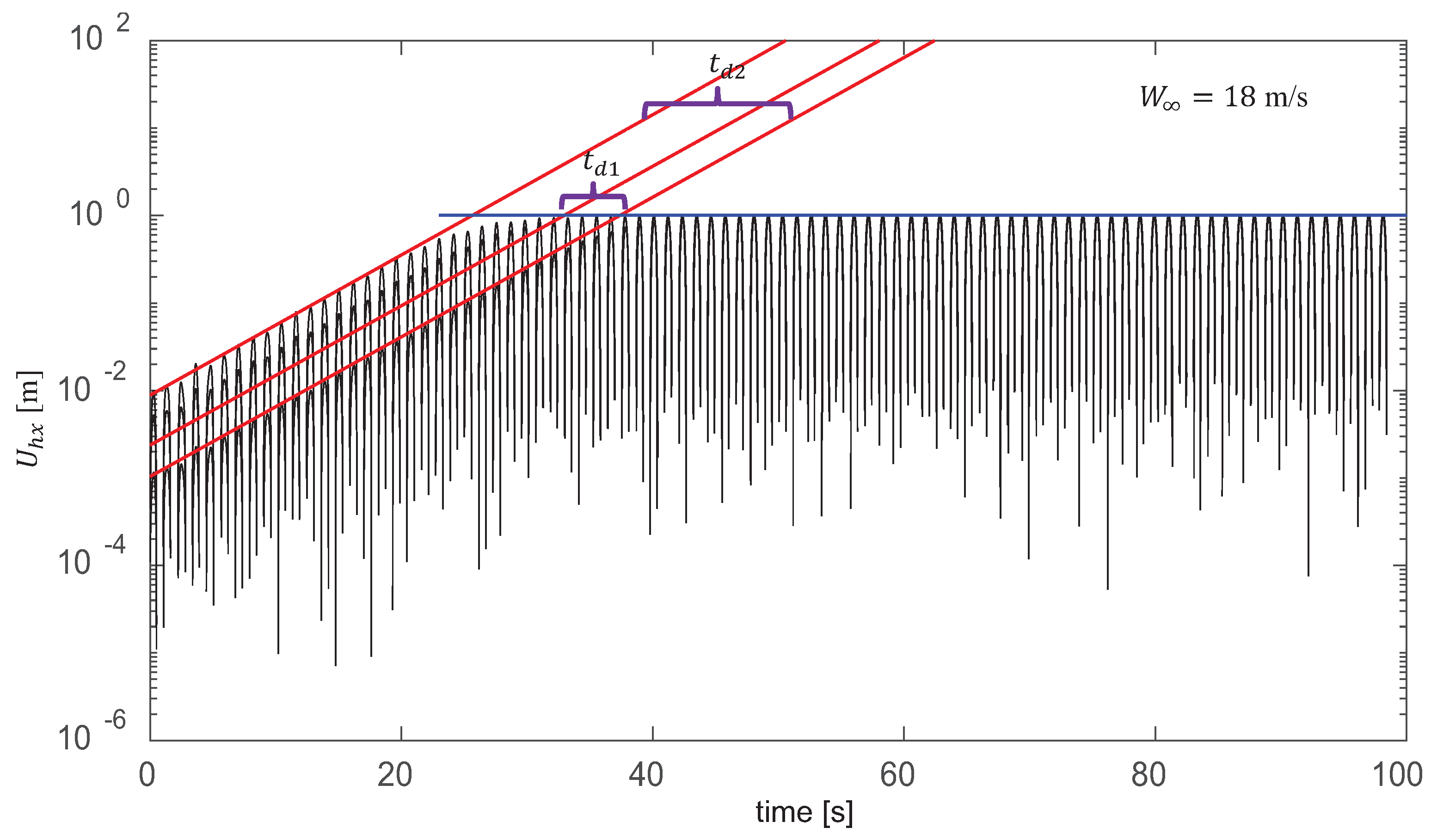
• Short pulses (associated with wind flow turbulence): These are characterized by pulses that are short enough that they end before the first peak in the blade oscillation occurs. After a very short initial time when the blades start displacing and accumulating energy by their own inertia, they deflect to a maximum, and the kinetic energy content of the wind pulse is accumulated as blade elastic deformation. The energy transfer and subsequent evolution can be characterized only by measuring the instantaneous blade deflection.
• Pulse-duration transitional zone: This is characterized by pulses that are long enough that energy dissipation by aerodynamic damping occurs during the duration of the pulse itself (i.e., only part of the pulse energy goes into elastic energy). Energy transfer and evolution can no longer be characterized only by measuring blade deflection.
• Long pulses: These are characterized by pulses that are long enough that they act as gradual variations in the kinetic energy of the flow that are absorbed by the rotor, inducing very small (or even negligible) oscillations.

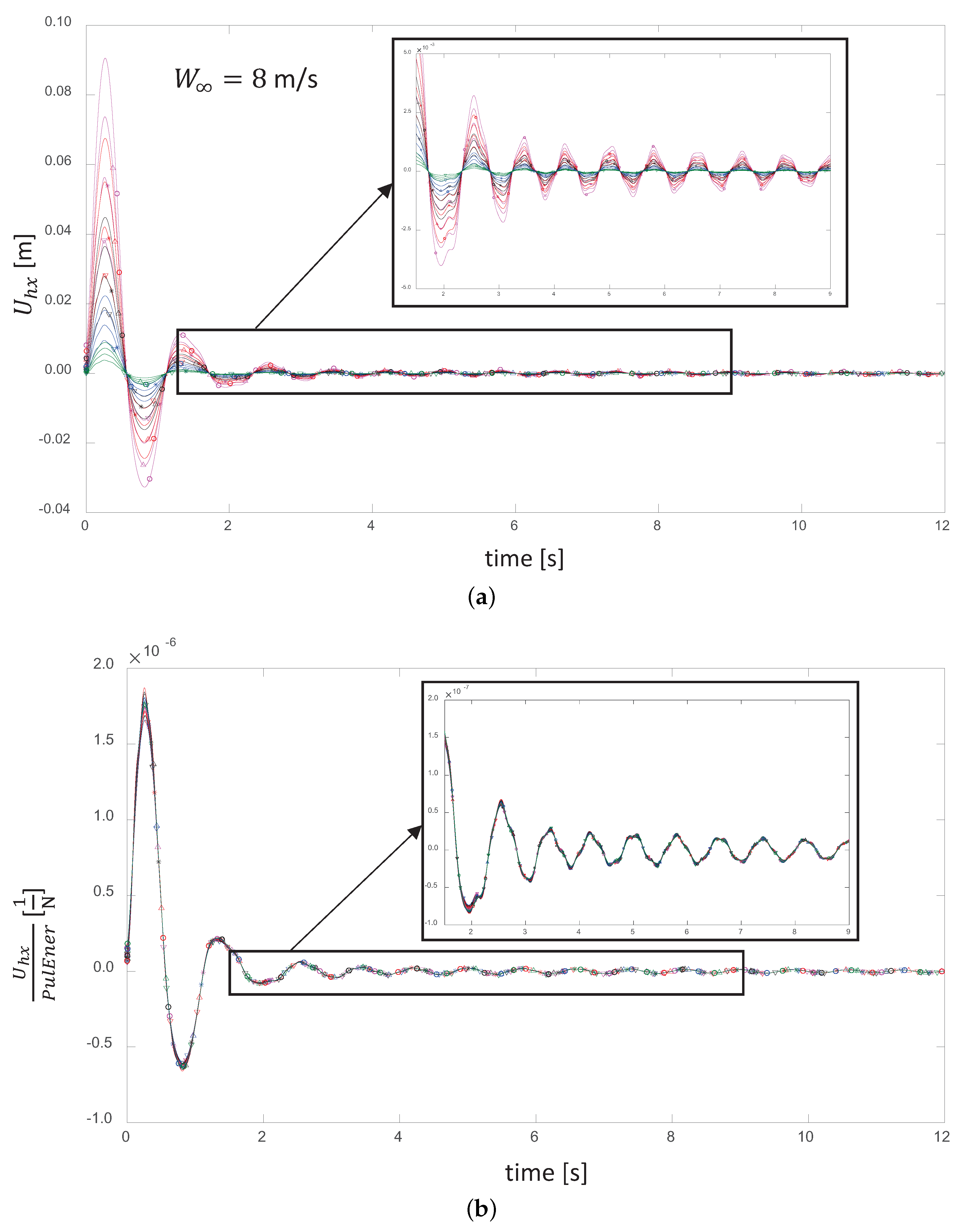
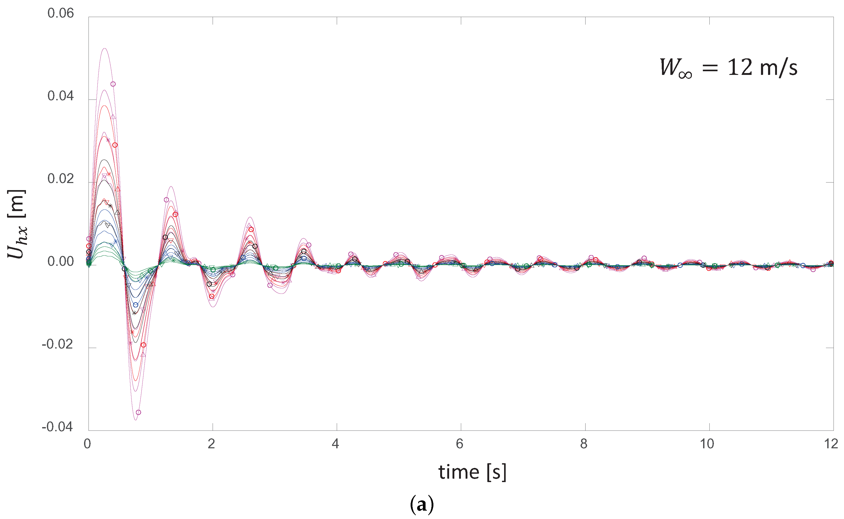
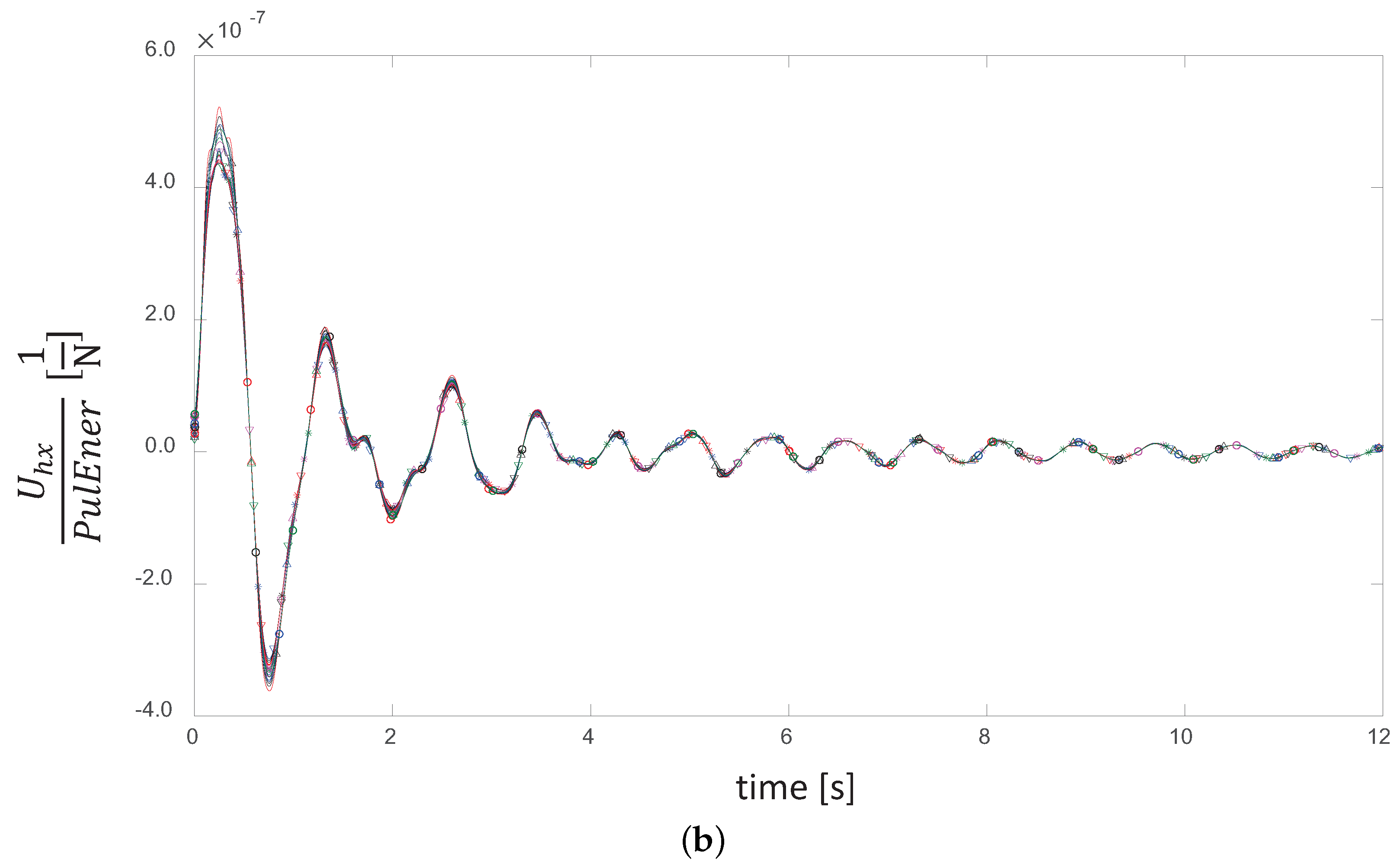
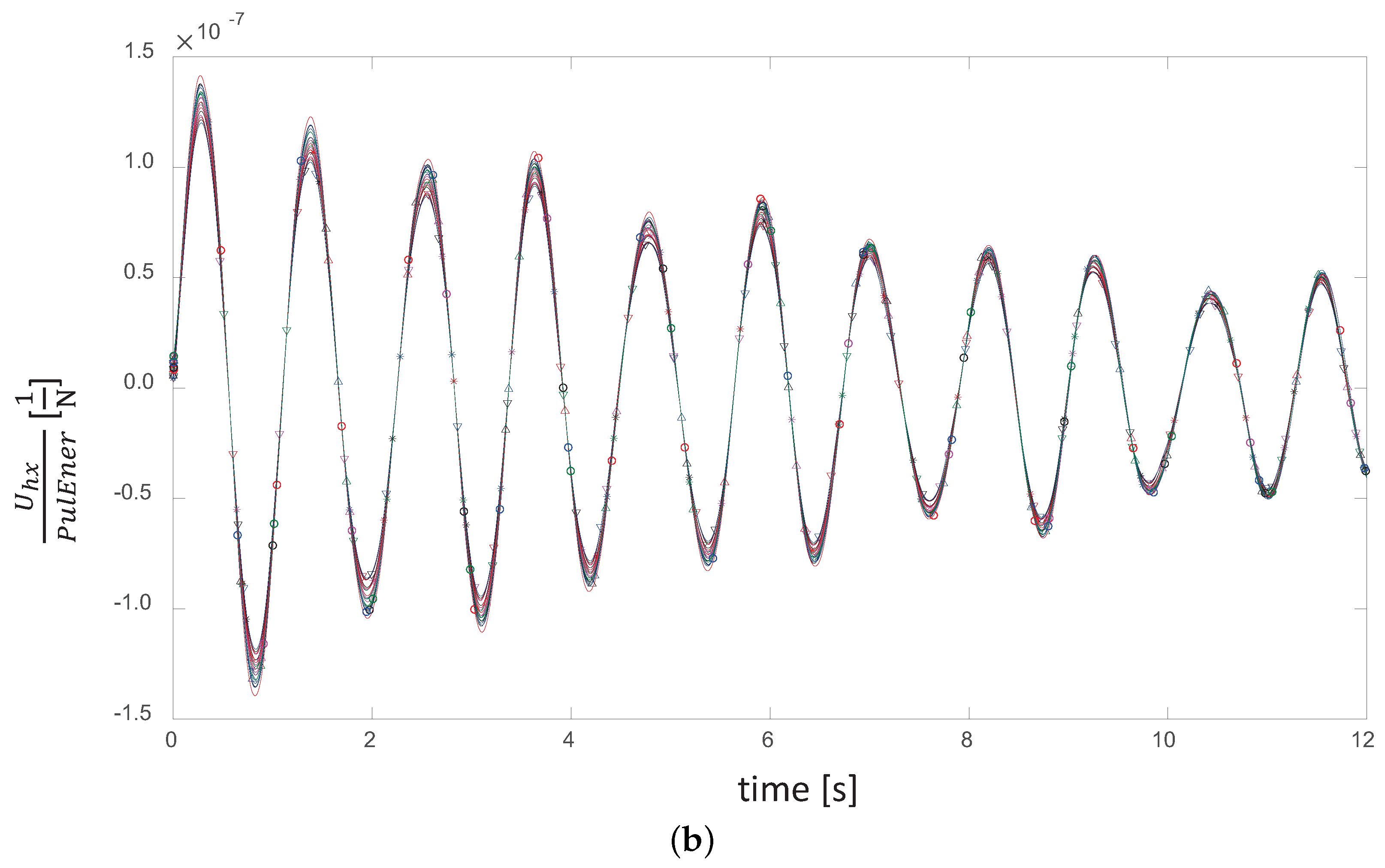
4. Energy-Transfer Characterization of the Pulse (Stable Oscillatory Regime)

The axial displacement of the blade $U_{hx}$ (depicted in Figure 5a for a wind-speed regime of 8 m/s) reflects the main component of the instantaneous amount of elastic energy stored in the rotor as an oscillatory system. We used it as an observable to construct a reduced-order characterization of the complex nonlinear oscillatory behaviors in terms of only one degree of freedom. We conducted this experiment for a wide variation of pulses in the short-duration zone, as in the classification chart shown in Figure 4, by combining different values of pulse amplitude and pulse time span. Figure 6 shows the code of the colors and markers used to identify the results for the pulses that combined different values of amplitude and time span.

When normalized by the kinetic energy content of the pulses, as shown in Figure 5b, all of the displacement curves collapse into a unique signal, which scales as the time evolution of the rotor’s elastic vibrational energy. This has the units of an equivalent flexibility, N${}^{-1}$, or the inverse of a stiffness $1/K_{el}$.

We repeated the same experiment for several wind speed conditions that covered the entire stable regime and found the same systematic behavior. For example, Figure 7 shows the results of the kinetic energy normalization for a wind speed of 12 m/s, and Figure 8 shows the results for a wind speed of 16 m/s. The value of the equivalent stiffness mentioned above, $K_{el}$, which serves as a scaling factor for the rotor’s elastic vibrational energy, depends exclusively on the mean wind speed. This is consistent with the average deflection of the blades around which the oscillations occur. The higher the mean wind speed is, the higher the value of this “pre-stiffening” will be.

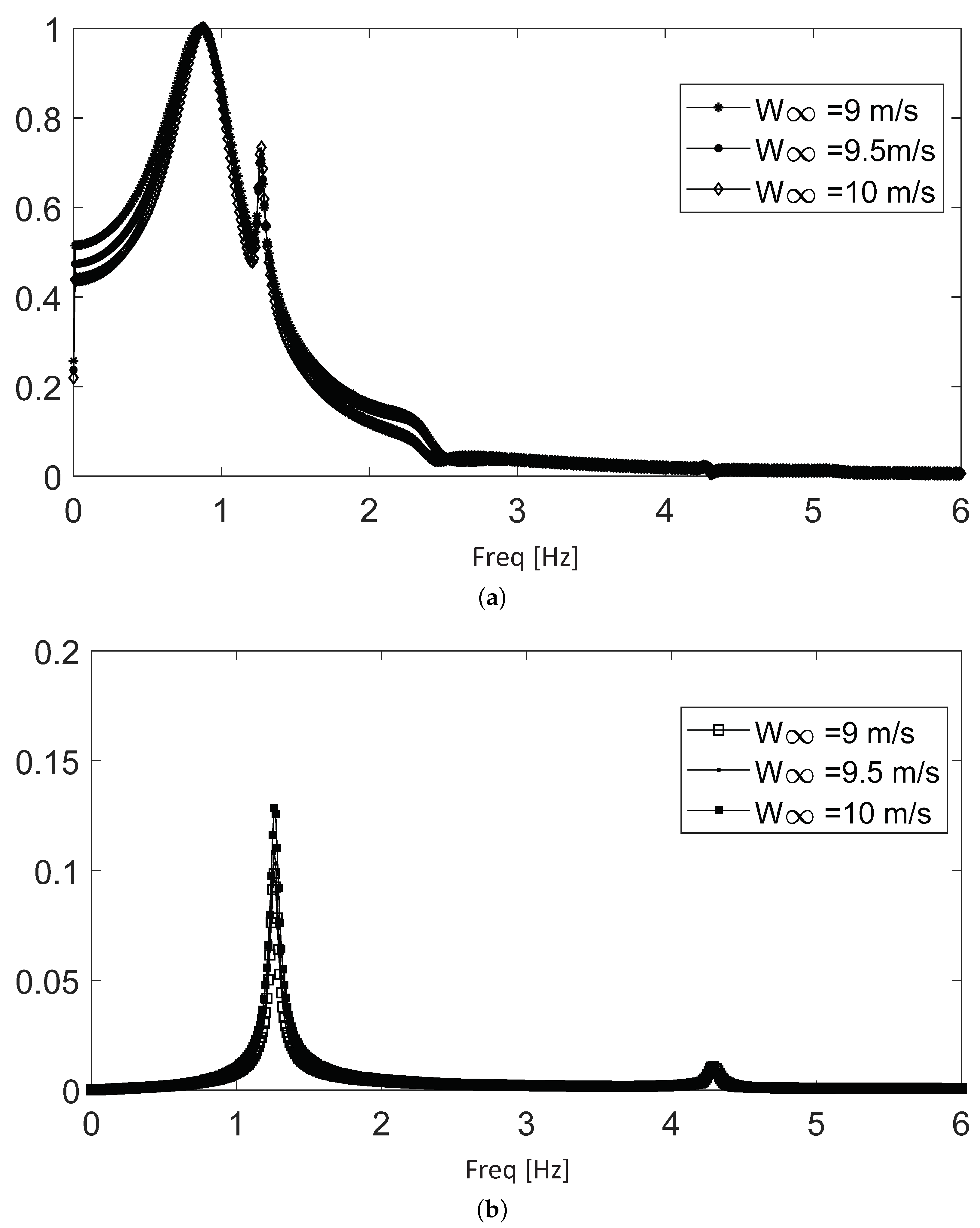
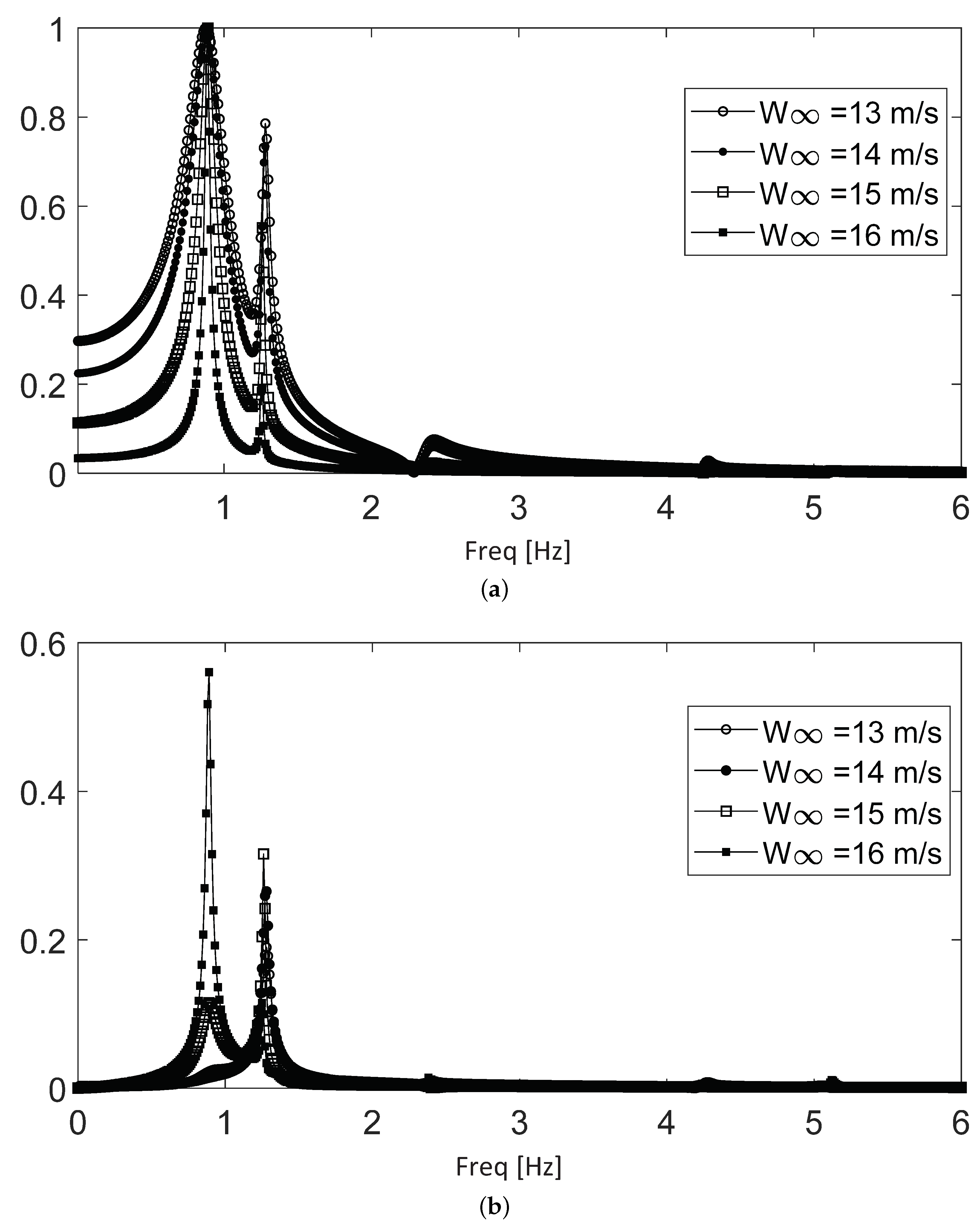
Frequency Content in the Stable Oscillatory Regime

In analyzing the frequency content in the stable regime, we found the appearance of five frequencies (only three of them were dominant), which showed different proportional contributions in four different subranges along the stable wind-speed range.

Figure 9 shows the spectra for the first subrange, which extends from 5 to 8 m/s, where only the first two frequencies (0.87 and 1.2 Hz) are dominant. The upper panel shows the frequency content along the time evolution (i.e., until oscillations are totally dissipated), where the 0.87 Hz frequency dominates, with a relatively small contribution of the 1.2 Hz frequency. The lower panel shows the spectrum for the long-term part of the same time signals. The 0.87 Hz frequency rapidly decays, while the 1.2 Hz component—even though it is smaller in the beginning—persists longer. In the long term, there is also a minimal contribution of the non-dominant 4.2 Hz frequency.

Figure 10 shows the spectra for the second subrange, which extends from 9 to 10 m/s. In this subrange, the 0.87 Hz frequency is dominant in the early stages, but the contribution of the 1.2 Hz frequency becomes more prominent. The long-term spectra for the same signals only show the 1.2 Hz component, which persists even longer than in the first subrange. Again, there is also a minimal contribution of the non-dominant 4.2 Hz frequency.

Figure 11 shows the spectra for the third subrange, which extends from 12.5 to 12.5 m/s. This subrange shows a much richer combination of the five frequencies observed, with three of them being dominant. Even though the 4.2 and 5.14 Hz components take a long time to decay, they are still not dominant. As before, the 0.87 Hz frequency is the most prominent, but the relative contribution of the 1.2 Hz component increases even more compared with the previous subranges. The most remarkable feature of this subrange is the emergence of a third dominant frequency of 2.4 Hz, which is particularly intense at 11 m/s. The 2.4 Hz frequency is only observed as a dominant component in this subrange specifically.

Figure 12 shows the spectra for the fourth and last subrange, which extends from 13 to 16 m/s, where the contribution is again mostly centered around the 0.87 Hz frequency, with a stronger presence of the 1.2 Hz component. An important distinctive feature is the presence of the 0.87 Hz frequency in the long-term spectra, which indicates a longer persistence (thus, a lower exponential decay) for this component. This ever-lower exponential decay of the 0.87 Hz component leads to the end of the stable regime, where the exponential decay approaches zero and then becomes negative. Thus, the aerodynamic damping turns into exponential expansion. In this subrange, the contributions of the other three frequencies become minimal.

When analyzing the semi-log plots of the oscillating signals, it becomes clear that their time evolution is characterized by an exponential enveloping curve, which is manifested as a linear relation when plotted in semi-log axes. Figure 13 shows three examples of semi-log plots of the time evolution of the normalized blade deflection at selected wind speeds in different subranges of the stable regime. In all of the panels, the short-term evolution, in which the 0.87 Hz frequency dominates, shows a greater exponential decay, ${\lambda }_1$, given by the slope of the red line. However, the lower exponential decay associated with the 1.2 Hz frequency, ${\lambda }_2$, becomes dominant in the long term. In the middle panel, we can see the contribution of the 2.4 Hz frequency overlapping with the 0.87 and 1.2 Hz components. By applying a bandpass filter to each one of the dominant components, the values of their corresponding exponential decays can be measured.

Figure 14 shows the variation of the exponential decay of the aerodynamic damping for the complete range of wind speeds in the stable oscillatory regime. The exponential decay associated with the 0.87 Hz frequency (${\lambda }_1$) shows a clear connection with the four different subranges associated with the frequency content that we have seen before.

The 1.2 Hz frequency shows an exponential decay that is much lower. Even though it has a lower amplitude in the mix of frequencies, it persists for a longer time, and that is the reason for why it is more prominent in the long-term spectra.

The 2.4 Hz frequency only appears in the third subrange, and it shows a sudden decrease in its exponential decay located at 11 m/s, which makes that component persist for a longer time. It returns to a higher dissipation rate at wind speeds of 12 m/s.

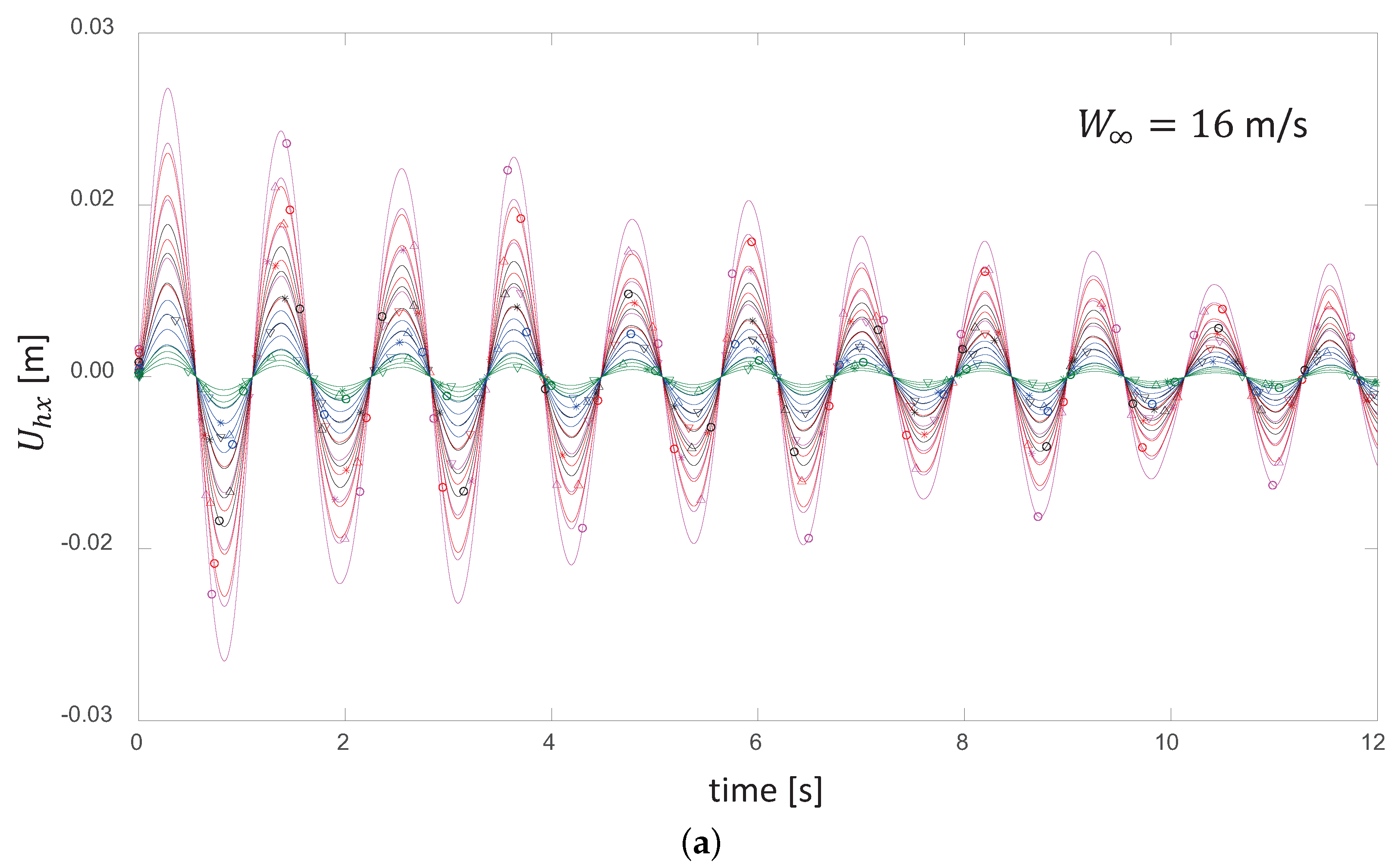
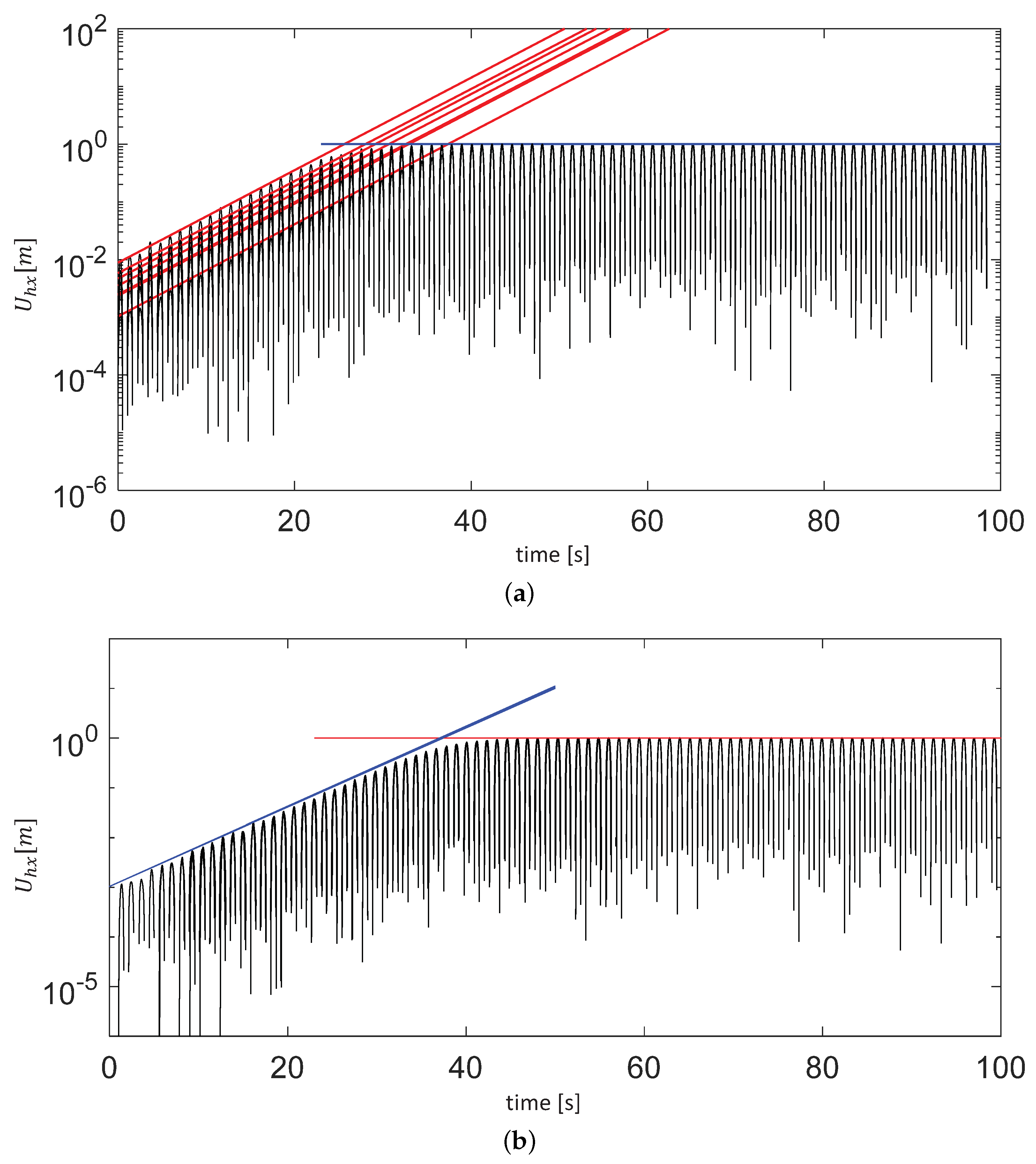
5. Energy-Transfer Characterization of the Pulse (Unstable Oscillatory Regime)

In the unstable regime, ${\lambda }_1$ becomes negative (that is, the attenuation of the aerodynamic damping becomes an amplification of the oscillatory amplitude), producing an initial exponential expansion that will be studied in detail in Section 5.1. The initial expansion continues until the axial displacement reaches a certain level. From then on, a second damping mechanism emerges that competes with the existing ${\lambda }_1$ amplification associated with the first mechanism. This evolution then starts to depart from the exponential behavior until the amount of energy extracted from the flow by the first mechanism is equivalent to that dissipated by the second. At that point, the oscillation levels out at a fixed amplitude. This effect shall be discussed in Section 5.2.

As in the stable regime, the axial displacement of the blade $U_{hx}$ around the equilibrium position (depicted in the upper panel in Figure 15 for a wind-speed regime of 18 m/s) reflects the main component of the instantaneous amount of elastic energy stored in the rotor as an oscillatory system. The time evolution of the blade deflection shows the same qualitative behavior for all of the wind speeds in this regime (17.5 to 25 m/s), but with different values of the initial exponential expansion. As in the stable regime, ${\lambda }_1$ depends exclusively on the mean wind speed.

The effect of the kinetic energy content of different pulses manifests as a delay in time, and all of the curves for a certain wind speed can be collapsed into one, as shown in the lower panel of Figure 15. That is, the pulse energy provides an initial threshold in the oscillation curve, and from then on, the oscillations continue feeding upon the energy of the mean flow. The delay time could be directly associated with the time required for the exponential expansion to build up the same amount of energy contained in their respective pulses by extracting it from the mean flow.

Figure 16 shows semi-log plots of the same time evolutions of the blade deflection previously shown in Figure 15. The initial expansion is exponential, which can be observed clearly in the linear shape of the initial enveloping curve in the semi-log plot. The enveloping curves of all of the pulses for the same mean wind speed show the same initial exponential coefficient ${\lambda }_1$, which becomes clear in the collapse of the curves for all of the pulses shown in the lower panel of Figure 16.

As mentioned before, all of the curves can be collapsed into one by shifting them by a certain delay time, $t_d$, which is associated with the time required for the exponential expansion to build up the same amount of energy contained in the respective pulse. As depicted in Figure 17, we took the curve for the pulse with the lowest energy (which is the pulse with the longest build-up) as a a time reference.

Then, the value of $t_d$ for each pulse can be directly computed by using the parameters obtained by fitting each pulse’s exponential curve. Equations (1) through (5) show the evaluation of $t_d$ by equating the exponential expression for each individual pulse with the exponential expression for the reference pulse (that is, collapsing the curves for all of the pulses).

$$U_h=A_0{e}^{-{\lambda }_1(t_{ref}-t_d)}$$

(1)

$$U_{h_{ref}}=A_{0_{ref}}{e}^{-{\lambda }_1{t}_{ref}}$$

(2)

$$A_{0_{ref}}{e}^{-{\lambda }_1{t}_{ref}}=A_0{e}^{-{\lambda }_1(t_{ref}-t_d)}$$

(3)

$$\frac{A_{0_{ref}}}{A_0}=\frac{e^{(-{\lambda }_1{t}_{ref}+{\lambda }_1{t}_d)}}{e^{-{\lambda }_1{t}_{ref}}}$$

(4)

$$t_d=\frac{1}{{\lambda }_1}Ln\left(\frac{A_{0_{ref}}}{A_0}\right)$$

(5)

5.1. Validation for the Unstable Regime of the Hypothesis Connecting the Time Delay and the Kinetic Energy Content of the Pulse

In order to validate the hypothesis that the time delay, $t_d$, is indeed associated with the time required for the exponential expansion to build up the same amount of energy contained in the respective pulse, we analyzed the relationship between two parameters: pulse kinetic energy and time delay. In this derivation, we also validate the hypothesis that the energy-transfer mechanism is exactly the same as in the stable regime, but with a negative value of ${\lambda }_1$, i.e., an amplification instead of attenuation of the oscillatory blade deflection. We shall start by combining Equations (1) and (2):

$$U_h=A_0{e}^{-{\lambda }_1(t_{ref}-t_d)}=A_0{e}^{-{\lambda }_1{t}_{ref}}{e}^{-{\lambda }_1{t}_d}=U_{h_{ref}}{e}^{-{\lambda }_1{t}_d}$$

(6)

$$\frac{U_h}{U_{h_{ref}}}=e^{{\lambda }_1{t}_d}$$

(7)

From the findings about the energy-transfer mechanism in the previous section, we have that, when normalized by the kinetic energy of the pulse, the blade displacement curves collapse into a unique signal, which scales with the time evolution of the rotor’s elastic vibrational energy. This has the units of flexibility or the inverse of stiffness $1/K_{el}$, which depends exclusively on the mean value of the wind speed. Hence, for all of the pulses occurring at the same wind speed, we have:

$$\frac{U_h}{PulsEner}=1/K_{el}=\frac{U_{h_{ref}}}{PulsEne{r}_{ref}}$$

(8)

$$\frac{PulsEner}{PulsEne{r}_{ref}}=\frac{U_{h_{ref}}}{U_h}$$

(9)

Equating expressions (7) and (9), we finally obtain:

$$\frac{PulsEner}{PulsEne{r}_{ref}}=e^{\left({\lambda }_1{t}_d\right)}$$

(10)

$$Ln\left(\frac{PulsEner}{PulsEne{r}_{ref}}\right)={\lambda }_1{t}_d$$

(11)

According to Equation (11), if the mechanism of energy transfer found earlier for the stable regime also holds for the unstable regime, the logarithm of the ratio between the kinetic energy of any pulse versus the energy of the reference pulse occurring at the same mean wind speed must show a linear relationship with the corresponding time delay for that same pulse, and the slope of that linear relation must be the value of ${\lambda }_1$ at that wind speed.

Figure 18 shows a plot of the logarithm of the kinetic energy ratio in Equation (11) versus the time delay for wind speeds covering the entire unstable regime. It can be seen that the values for all of the pulses show a very clear alignment with a linear relation, and least-squares fitting gives a value of ${\lambda }_1$ for each wind speed, which is in very close agreement with the values obtained by the fitting of ${\lambda }_1$ in the exponential expansion stage of $U_{hx}$ from the semi-log plots. Figure 19 shows a plot of ${\lambda }_1$ obtained with these two methods for the complete range of wind speeds in the unstable oscillatory regime.

The coincidence of the value of ${\lambda }_1$ obtained from these two different methods—one measuring the expansion as it progresses in time, and the other evaluating the time that would have been taken for the same expansion to build the same energy delivered by the pulse—proves that the time delay, $t_d$, is indeed associated with the time required for the exponential expansion to build up the same amount of energy contained in the respective pulse. This also validates the hypothesis that the energy-transfer mechanism is exactly the same as in the stable regime.

5.2. Stabilization of the Oscillatory Amplitude of the Unstable Regime

As mentioned before, the amplitude of the $U_{hx}$ oscillations shows evidence of the presence of a second dissipative mechanism that acts in parallel with the one associated with (the now amplifying) ${\lambda }_1$. This second dissipative mechanism also seems to be aeroelastic in nature, and it starts acting when the amplitude reaches a certain threshold that depends exclusively on the value of the uniform-stream wind speed, regardless of the nature of the pulse that triggered the oscillations in the first place.

In the same manner, there is another threshold in the amplitude value at which the rate of energy dissipation associated with the second aeroelastic mechanism equates the rate of energy influx from the first physical mechanism associated with ${\lambda }_1$ in such a manner that the oscillation amplitude levels out into a constant value. This stabilization threshold also depends exclusively on the wind speed.

Figure 20 shows an example of the oscillatory signal at 18 m/s, indicating the threshold at which the enveloping curve starts departing from the exponential behavior, $Dep\_U_h$, and the threshold at which the amplitude levels out into a stable regime, $SS\_U_h$. It also shows the values of these two thresholds for the whole range of wind speeds corresponding to the unstable regime.

6. Concluding Remarks

In our current work, we studied the pure aero-elasto-inertial dynamics of stall-controlled wind turbine rotors as oscillatory systems. We presented the results from an extensive series of experiments analyzing the dynamic response of the rotor to wind speed fluctuations associated with the turbulent characteristics of the atmospheric boundary layer, thus obtaining a reduced-order characterization based on energy-transfer principles.

In addition to its intrinsic scientific value, this aspect of the work presented here is of fundamental interest to researchers and engineers working on developing optimized control strategies for wind turbines. It allows for the critical elements of the rotor’s dynamic behavior to be described by a reduced-order model that can be solved in real time, an essential requirement for determining predictive control actions. These are critical in terms of mitigating peak structural loads, the stability of a turbine’s operational parameters, such as torque and power output, and reducing the accumulation of fatigue efforts.

As an outlook for further work, we envision a series of experiments exploring the dynamics of a rotor when subjected to wind-speed pulses of longer durations. Contrary to what happens with the short pulses associated with the turbulent content of the wind flow, for long pulses, the kinetic energy content of a pulse is delivered during a period of time that is comparable to or even longer than the period of the first peak of the displacement oscillation. Consequently, the aerodynamic damping has time to act during the duration of the pulse itself, dissipating a non-negligible part of the energy of the gust pulse before it becomes accumulated as elastic energy in the blade deflection. In this range of time scales of longer pulses, the energy-transfer principle is still expected to operate, but with the evolution of the blade-deflection peaks evolving in a different manner.

References

1. Fichaux, N.; Beurskens, J.; Jensen, P.H.; Wilkes, J.; Frandsen, S.; Sorensen, J.; Eecen, P.; Malamatenios, C.; Gomez, J.; Hemmelmann, J.; et al. Upwind: Design limits and solutions for very large wind turbines. Sixth Framew. Programme 2011, 1037, 042020. [Google Scholar]
2. Lalor, G.; Mullane, A.; O’Malley, M. Frequency control and wind turbine technologies. IEEE Trans. Power Syst. 2005, 20, 1905–1913. [Google Scholar] [CrossRef]
3. Senjyu, T.; Sakamoto, R.; Urasaki, N.; Funabashi, T.; Fujita, H.; Sekine, H. Output power leveling of wind turbine generator for all operating regions by pitch angle control. IEEE Trans. Energy Convers. 2006, 21, 467–475. [Google Scholar] [CrossRef]
4. Barlas, T.K.; Van Kuik, G.A.M. State of the art and prospectives of smart rotor control for wind turbines. In Journal of Physics: Conference Series; IOP Publishing: Bristol, UK, 2007; Volume 75, p. 012080. [Google Scholar]
5. Wingerden, J.W.V.; Hulskamp, A.W.; Barlas, T.; Marrant, B.; Kuik, G.A.M.V.; Molenaar, D.P.; Verhaegen, M. On the proof of concept of a ‘smart’ wind turbine rotor blade for load alleviation. Wind. Energy 2008, 11, 265–280. [Google Scholar] [CrossRef]
6. Bianchi, F.D.; De Battista, H.; Mantz, R.J. Wind Turbine Control Systems: Principles, Modelling and Gain Scheduling Design; Springer Science & Business Media: Berlin/Heidelberg, Germany, 2006. [Google Scholar]
7. Muljadi, E.; Pierce, K.; Migliore, P. Control strategy for variable-speed, stall-regulated wind turbines. In Proceedings of the 1998 American Control Conference. ACC (IEEE Cat. No.98CH36207), Philadelphia, PA, USA, 26 June 1998; Volume 3, pp. 1710–1714. [Google Scholar]
8. Muljadi, E.; Butterfield, C.P. Pitch-controlled variable-speed wind turbine generation. IEEE Trans. Ind. Appl. 2001, 37, 240–246. [Google Scholar] [CrossRef] [Green Version]
9. Polinder, H.; Bang, D.; van Rooij, R.P.J.O.M.; McDonald, A.S.; Mueller, M.A. 10 MW Wind Turbine Direct-Drive Generator Design with Pitch or Active Speed Stall Control. In Proceedings of the 2007 IEEE International Electric Machines & Drives Conference, Antalya, Turkey, 3–5 May 2007; Volume 2, pp. 1390–1395. [Google Scholar]
10. Bottasso, C.L.; Croce, A.; Gualdoni, F.; Montinari, P. Load mitigation for wind turbines by a passive aeroelastic device. J. Wind. Eng. Ind. Aerodyn. 2016, 148, 57–69. [Google Scholar] [CrossRef] [Green Version]
11. Menezes, E.J.N.; Araújo, A.M.; da Silva, N.S.B. A review on wind turbine control and its associated methods. J. Clean. Prod. 2018, 174, 945–953. [Google Scholar] [CrossRef]
12. Lubosny, Z.; Bialek, J.W. Supervisory control of a wind farm. IEEE Trans. Power Syst. 2007, 22, 985–994. [Google Scholar] [CrossRef]
13. Thresher, R.; Schreck, S.; Robinson, M.; Veers, P. Wind Energy Status and Future Wind Engineering Challenges; Technical Report NREL/CP-500-43799; National Renewable Energy Lab: Jefferson County, CO, USA, 2008.
14. Ponta, F.L.; Otero, A.D.; Lago, L.I.; Rajan, A. Effects of rotor deformation in wind-turbine performance: The Dynamic Rotor Deformation Blade Element Momentum model (DRD–BEM). Renew. Energy 2016, 92, 157–170. [Google Scholar] [CrossRef] [Green Version]
15. Yu, W.; Hodges, D.H.; Volovoi, V.; Cesnik, C.E.S. On Timoshenko-like modeling of initially curved and twisted composite beams. Int. J. Sol. and Struct. 2002, 39, 5101–5121. [Google Scholar] [CrossRef]
16. Hodges, D.H. Nonlinear Composite Beam Theory; AIAA: Reston, VA, USA, 2006. [Google Scholar]
17. Otero, A.D.; Ponta, F.L. Structural Analysis of Wind-Turbine Blades by a Generalized Timoshenko Beam Model. J. Sol. Energy Eng. 2010, 132, 011015. [Google Scholar] [CrossRef]
18. Menon, M.; Ponta, F. Dynamic Aeroelastic Behavior of Wind Turbine Rotors in Rapid Pitch-Control Actions. Renew. Energy 2017, 107, 327–339. [Google Scholar] [CrossRef] [Green Version]
19. Otero, A.D.; Ponta, F.L. On the sources of cyclic loads in horizontal-axis wind turbines: The role of blade-section misalignment. Renew. Energy 2018, 117, 275–286. [Google Scholar] [CrossRef]
20. Jonkman, J.; Butterfield, S.; Musial, W.; Scott, G. Definition of a 5-MW Reference Wind Turbine for Offshore System Development; Technical Report NREL/TP-500-38060; National Renewable Energy Laboratory: Jefferson County, CO, USA, 2009.
21. Xudong, W.; Shen, W.Z.; Zhu, C. Shape optimization of wind turbine blades. Wind Energy 2009, 12, 781–803. [Google Scholar] [CrossRef]
22. Jalal, S.; Ponta, F.; Baruah, A. Aeroelastic Response of Variable-Speed Stall-Controlled Wind Turbine Rotors. In ASME 13th International Conference on Energy Sustainability; American Society of Mechanical Engineers: New York, NY, USA, 2019. [Google Scholar]
23. Jaimes, O.G. Design Concepts for Offshore Wind Turbines: A Technical and Economical Study on the Trade-Off between Stall and Pitch Controlled Systems. Ph.D. Thesis, Delft University of Technology, Delft, The Netherlands, 2010. [Google Scholar]
Figure 1. An example of a wind-speed pulse stimulus of controlled amplitude and time span.
Applsci 11 06886 g001
Figure 2. Examples of the time evolution of the axial component of the blade deflection at wind speeds (a) below and (b) above the wind speed stability threshold.
Applsci 11 06886 g002
Figure 3. Examples of the time evolution of the axial component of the blade deflection at wind speeds on the narrow range of the transitional regime. (a) lower end of the transitional range, and (b) higher end of the transitional range.
Applsci 11 06886 g003
Figure 4. Amplitude versus characteristic time span chart for typical oscillations in wind speed.
Applsci 11 06886 g004
Figure 5. (a) Time evolution of the axial displacement of the blade at a wind-speed regime of 8 m/s for pulses that combine different values of amplitude and time span. (b) The same curves normalized by the kinetic energy content of their respective pulses.
Applsci 11 06886 g005
Figure 6. Code of colors and markers used to identify the results for pulses that combine different values of amplitude and time span.
Applsci 11 06886 g006
Figure 7. (a) Time evolution of the axial displacement of the blade at a wind-speed regime of 12 m/s for pulses that combine different values of amplitude and time span. (b) The same curves normalized by the kinetic energy content of their respective pulses.
Applsci 11 06886 g007aApplsci 11 06886 g007b
Figure 8. (a) Time evolution of the axial displacement of the blade at a wind-speed regime of 16 m/s for pulses that combine different values of amplitude and time span. (b) The same curves normalized by the kinetic energy content of their respective pulses.
Applsci 11 06886 g008aApplsci 11 06886 g008b
Figure 9. Frequency spectra for the first subrange along the stable regime. (a) Complete time evolution. (b) Long-term evolution.
Applsci 11 06886 g009
Figure 10. Frequency spectra for the second subrange along the stable regime. (a) Complete time evolution. (b) Long-term evolution.
Applsci 11 06886 g010
Figure 11. Frequency spectra for the third subrange along the stable regime. (a) Complete time evolution. (b) Long-term evolution.
Applsci 11 06886 g011
Figure 12. Frequency spectra for the fourth subrange along the stable regime. (a) Complete time evolution. (b): Long-term evolution.
Applsci 11 06886 g012
Figure 13. Semi-log plots of the time evolution of the normalized blade deflection at selected wind speeds in different subranges of the stable regime. The red and blue lines indicate the enveloping curves for the decaying components of the signal associated with the first (0.88 Hz) and second (1.2 Hz) frequencies respectively.
Applsci 11 06886 g013
Figure 14. Variation of the exponential decay of the aerodynamic damping for the complete range of wind speeds in the stable oscillatory regime.
Applsci 11 06886 g014
Figure 15. (a) Time evolution of the axial displacement of the blade at a wind-speed regime of 18 m/s for pulses combining different values of amplitude and time span. (b) The same curves, but delayed in time for the exponential expansion to build up the same amount of energy contained in their respective pulses.
Applsci 11 06886 g015
Figure 16. (a) Time evolution of the axial displacement of the blade at a wind-speed regime of 18 m/s for pulses combining different values of amplitude and time span. (b) The same curves, but delayed in time for the exponential expansion to build up the same amount of energy contained in their respective pulses. The red and blue lines indicate respectively the enveloping curves for the exponential component and maximum amplitudes of the different signals.
Applsci 11 06886 g016
Figure 17. Time delay for each pulse, taking the curve for the pulse with the lowest energy as a time reference. The red lines indicate the enveloping curves for the exponential component of the different signals.
Applsci 11 06886 g017
Figure 18. Logarithm of the kinetic energy ratio for different pulses occurring at the same mean wind speed versus the pulse time delay for wind speeds covering the entire unstable regime.
Applsci 11 06886 g018
Figure 19. Comparative plots of λ 1 versus the mean wind speed for the complete range of wind speeds in the unstable oscillatory regime, which was obtained through a direct fitting on the exponential expansion stage of U h x from the semi-log plots and from the energy-transfer relation in Equation (11).
Applsci 11 06886 g019
Figure 20. An example of the oscillatory signal at 18 m/s indicating the D e p _ U h and S S _ U h thresholds and the values of these thresholds for wind speeds in the unstable regime.
Applsci 11 06886 g020
Publisher’s Note: MDPI stays neutral with regard to jurisdictional claims in published maps and institutional affiliations.