Impact of a Robot Manipulation on the Dimensional Measurements in an SPC-Based Robot Cell

Abstract

In our study a robot was used to deliver objects for measurement into the Equator gauging system. To investigate the robot’s manipulation influence on dimensional measurements, the robot’s tasks were divided into basic functions. Based on these basic functions, nine different robot-manipulation scenarios were defined, i.e., from zero to full robot manipulation, for two measuring objects (named Magnet and PKR) and six measurement characteristics (rectangular and spherical). The robot’s manipulation influence was determined on the basis of the statistical parameters $C_p$, R, and the $6\sigma$ obtained from a measurement system analysis (MSA) type-1 study. The results show that the degree of implemented manipulation of the robot affects the scattering of the measurement data. However, the effect is much more pronounced in the case of length measurements than with spherical geometries. Different measuring methods (touch-triggering or scanning measurement mode, number of sampling points) were used, which showed similar measurement data. This directly indicated the influence of the robot’s manipulation on $C_p$, R and $6\sigma$. Increasing the degree of the robot’s manipulation decreases the $C_p$ value and increases the R and $6\sigma$ values for the length measurements. There is no such pronounced course in the spherical geometries, where the values of $C_p$, R and $6\sigma$ remain approximately the same. The main influential factor for decreasing the $C_p$ value with increasing robot manipulation was the angular misalignment of the object’s orientation in the fixture.

1. Introduction

Recently, there has been an increasing emphasis on product-quality and process control in the process industry. Due to the increasing daily demands for better product quality, the need for ever-improving measuring systems is also on the increase.

Several different approaches are used to ensure adequate quality and process control. The most commonly used method in manufacturing is Statistical Process Control (SPC) [1,2]. Amongst SPC techniques (histograms, control charts, scatter diagrams, etc.), there are methods for evaluating the manufacturing process’s capability (including the capabilities of the measuring system).

Coordinate measuring machines (CMMs) have a leading role in manufacturing metrology because of their versatile and flexible use. However, in addition to these good qualities, they also possess some important disadvantages. They are costly, in many cases, time-consuming, and they require temperature-controlled rooms to achieve their optimum measurement capabilities. Many potential sources are able to influence CMMs’ measurement uncertainties, most notably the environment of the measurements, the measurement procedure [3,4,5,6,7,8,9,10,11,12,13,14,15,16], the measuring equipment [3,9,10,11,14,15], and the operator [3,4].

The operator influences process measurements through conscious or unconscious actions. Using different measuring tools, the operator can apply forces of different sizes (e.g., measuring lengths or diameters when using calipers). When holding the object in clamps for measurements with a CMM, the operator can cause deformations of the measured object or introduce uncertainty due to a positioning error. Unlike operators (in general, humans), industrial robots have much better repeatability and accuracy of their movements. Besides, they can operate continuously without stopping. In this regard, robots can be used in place of operators and increase the data’s reliability, and, at the expense of continuous operation, the sample of measured objects can be increased. These days, robots also allow for a reasonable degree of flexibility.

Numerous studies have been conducted to speed up the measurements involving industrial robots, laser scanners, and optical CMMs [17,18,19,20]. Kirachi et al. [17,18] and Altinisik [19] compared CMMs with laser scanners attached to industrial robots in the automobile industry. In all cases, the measurement cycle time was significantly reduced compared to CMM measurements. Additionally, the density of measured points was increased. However, it should be noted that it was not possible to measure all the characteristics using the combination of a robot and a laser scanner, and the method is suitable for measuring relatively large subjects (e.g., car chassis) with a tolerance of 3 mm (±1.5 mm).

Lemes et al. [20] used an industrial robot to manipulate a measured object inside the CMM’s working area. The main goal of the research was to perform the re-positioning of a measured object with a 5-axis industrial robot and fully automate the measurement cycle. They concluded that it is possible to conduct measurements using a CMM-robot system. However, the measurement results are dictated by the measurement uncertainty of the least-accurate component of the system, an industrial robot in this case.

Measurement uncertainty that encompasses the operator’s influence can be significantly reduced by changing the measurement methods appropriately. The operator’s influence includes the determination of the measurement probes and stylus [12], the sampling method [6,7,8,13] for the measured features (distribution and number of points), and the positioning of the part and fitting algorithms [9,10,11]. As demonstrated in Reference [20], with some additional improvements, the uncertainty part due to the positioning error can be reduced. Nevertheless, Papananias et al. [21], Forbes et al. [14], and Forbes et al. [22] showed that using a CMM in comparator mode eliminates the kinematic part of the measurement uncertainty and reduces the part associated with environmental impacts. Systematic effects associated with the measurement system apply both to the measurements of the test artefact and the master artefact, and a substantial proportion of the systematic effect associated with the two sets of measurements cancel out.

In industry, there have already been demonstrations of an automated measurement system with a reduced influence of the operator. However, the current literature does not present automated solutions that would involve a combination of a robot and contact measurements where the robot would replace the operator to serve the measuring machine (including object grasping and manipulation, insertion, and removal).

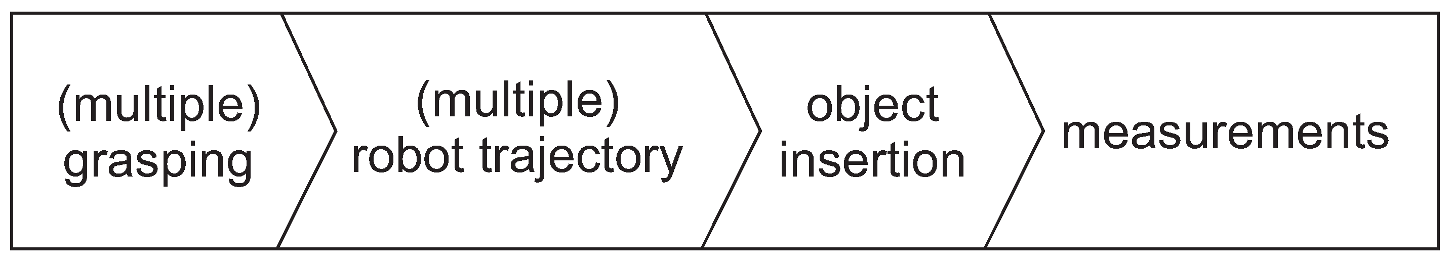
This work investigates another previously unstudied, but today important, dimension to show how the measurement outcome varies during automation. More specifically, we are interested in the influence of the robot’s manipulation (that occurs before a dimensional measurement) on the object’s final dimensional measurements. More in detail, measurement data scattering. We identified some important and problematic robot manipulation actions that affected the scattering of dimensional measurement data. We divided actions into grasping, robot trajectory, object insertion, and measurements (Figure 1). Furthermore, object insertion can be divided into translation and rotation. Meanwhile, robot trajectory can be divided into linear and joint motions. Figure 1 also shows that multiple grasps, as well as several trajectory sections, appear in regular manipulation to measurement cycle. The measurement itself is ultimately the last phase, which means that all previous grasping or manipulation actions might influence 6D pose repeatability of the measured part. The geometry of the measured part is not ideal. Inherited are many dimensional tolerances that mirror better measurement system analysis (MSA) parameters [23,24] if repeatability in all previous steps is high. In the case of poor repeatability, we, indeed, measure different points with different tolerances on the object. Advanced use-case examples of robots are the core pillars of Industry 4.0 and quality assurance, with both gaining importance in a product-adaptive or modularly composed environment. In this way, such a question is essential for state-of-the-art Industry 4.0.

The primary role of quality assurance is elementary, i.e., always measure in the same way. This is not the case if the robot’s handling of the object is not constant, something that would introduce more variability into the measurement procedure. For instance, the manipulator mechanics of an old robot, with many working hours or loose grasping, add more and more positional and rotational uncertainty to an otherwise “constant” robot’s individual actions and set of movements. Finally, this leads to positional and orientational (i.e., relating to the pose) uncertainty of the measured object [25,26]. Pose uncertainty influences the measuring equipment’s capability, as well as the repeatability and reproducibility, which are all well-defined for today’s acknowledged quality-assurance producers (see Section 2).

The influence of robot manipulation on the capability of measuring systems is studied for nine different robot scenarios. The robot provides complex and straightforward object handling, while the Equator (parallel robot) contact measuring device is used for the measurement. The initial assumption that a higher degree of robot manipulation directly affects the capability factor $C_p$ is verified and confirmed. It turns out that the sampling strategy and measurement method (scanning and touch-triggering mode) have a much smaller impact on the capability factor $C_p$ than the robot grasping and the manipulation itself. Normal distribution of grasping, manipulation and measurement data is confirmed. Using appropriate sequences, the MSA statistical parameters can be improved.

The rest of the article is organized as follows. Different capability indices used in industry are presented in Section 2. Section 3 describes the measurement system and the equipment. Nine robot scenarios are introduced with measured objects and their measured characteristics. The results are presented in Section 4 and discussed in Section 5. Concluding remarks are given in Section 6.

2. Process Capability—Capability Indices

To quantify process capability, a statistical analysis of the process itself, considering the process mean $\mu$ and the standard deviation $\sigma$, has to be taken into account. Normally, $\mu$ and $\sigma$ are unknown and approximated by $\overline{x}$ and s, respectively. For a statistical evaluation, several capability indices are used in manufacturing, such as precision-to-tolerance (PTR) [27,28,29,30,31,32,33,34], number of distinct categories (NDC) [28,34], repeatability and reproducibility (R&R) [31,34,35], and discrimination ratio (DC) [34,35]. The indices can be roughly divided into two subgroups for:

• comparing the tolerance of the part’s specifications with the measurement system’s variability ${\sigma }_m$, and
• matching the process variability ${\sigma }_p$ to the measurement system’s variability.

The PTR is the most commonly used criterion concerning the first group because of its simplicity. It represents the percentage of tolerance consumed by the variability of the measurement. The general form is shown in (1), where k is a constant and corresponds to the limiting number of standard deviations. Normally, k equals 6.

$$PTR=\frac{k{\sigma }_m}{TOL}.$$

(1)

The NDC, the percentage of repeatability and reproducibility (%GR&R), and DC are the main criteria based on process and measurement variability. The NDC criterion is often reported as the signal-to-noise ratio (SNR).

The first group of capability indices should be taken into account during part inspection and measurement-system selection. In the case of process control, measurement-system selection has to be made using the second group’s criteria. In many cases, when the data from parts are used to determine the process variability, measurement-system selection must consider both groups of criteria simultaneously. In the literature, a lower PTR value than the threshold value (commonly set between 5% [36,37] and 10% [31]) indicates an acceptable measurement method. The NDC has the opposite behavior to that of the PTR. A larger value indicates a more acceptable measurement method, and the threshold value is commonly set to 5 [1,38]. It must be pointed out that there is no indication of how these thresholds were established.

Referencing the MSA study of References [23,24], a type-1 study corresponds to the capability of the measurement equipment (the measurement process) and type-2 and -3 studies correspond to a repeatability and reproducibility study (with and without the operator’s influence). The measurement equipment’s capability is commonly calculated as the $C_p$ factor, which is called the precision index and is calculated as:

$$\begin{array}{cc}\hfill C_p& =\frac{allowableprocessspread}{actualprocessspread}\hfill \\ \hfill & =\frac{TOL}{6{\sigma }_p}\hfill \\ \hfill & =\frac{USL-LSL}{6{\sigma }_p}\hfill \end{array}.$$

(2)

USL and LSL are the upper and lower specification limits. Due to its simplicity, $C_p$ cannot provide an assessment of the process centering. To measure the degree of process centering relative to the manufacturing tolerance, the accuracy index $C_a$ is defined as:

$$C_a=1-\frac{|\mu -m|}{d},$$

(3)

where $\mu$ is the process mean, $d=\frac{USL-LSL}{2}$ is the half specification width, and $m=\frac{USL+LSL}{2}$ is the midpoint between the upper and lower specification limits. As can be seen from (3), any deviation from the centered point results in a reduction of the $C_a$ value. Combining the $C_p$ and $C_a$ factors results in a definition of the $C_{pk}$ factor as:

$$C_{pk}=min\left\{\frac{USL-\mu }{3\sigma },\frac{\mu -LSL}{3\sigma }\right\}=\frac{d-|\mu -m|}{3\sigma }.$$

(4)

It must be noted that the use of the parameters $C_p$, $C_a$, and $C_{pk}$ requires a normal distribution of the measured data.

An MSA type-1 study evaluates the capability of a measuring process. In studies of type-2 and -3, it is the capability of the measuring process in terms of the verification of variation using measurements of the serial product (R&R—the repeatability and the reproducibility) with or without operator influence.

3. Materials and Methods

3.1. Measurement Equipment

For our study, we used an adaptive robotic cell (ARC) for automated SPC dimensional measurements developed in our laboratory in collaboration with the company Kolektor. The whole robotic cell consists of five modules, a module with a robot, a module with the Equator, a module for optical inspections, an accessory module with a storage area, and a module for the supply of subjects on measuring pallets. The ARC, therefore, makes possible contact and non-contact dimensional measurements. For our research, a subset of a module with a robot, a supply module, and a module with the Equator were used (Figure 2). The immediate observation was that the robot manipulation has a more significant influence on the variance of contact dimensional measurements than the non-contact dimensional measurements; therefore, non-contact methods were off the study.

In the ARC and this study, we used a collaborative robot UR5e manufactured by Universal Robots, with an attached CRG 30-050 collaborative servo gripper from Weiss Robotics. For the contact measurements, the comparator principle-based measurement system Renishaw Equator 300 was used. The primary task of the robot is to tend the Equator with measured objects into a fixture in the Equator’s working area. The robot was replicating the operator in traditional and manual measurements.

3.2. Measured Objects

For our study, we selected two types of serial product, i.e., a Magnet and a PKR. For each of the products, we implemented the measurement characteristics currently measured as part of the SPC measurements. 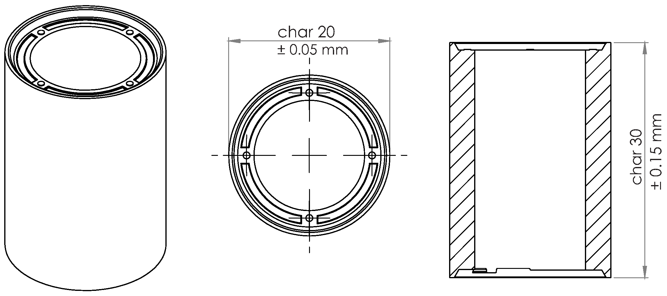In the case of the Magnet object, two characteristics were measured: (i) the characteristic diameter with code 20 and (ii) the characteristic height with code 30, with tolerances, respectively, $\pm 0.05\mathrm{mm}$ and $\pm 0.15\mathrm{mm}$ (Figure 3), and, in the case of the PKR object, four characteristics were measured: (i) the characteristic height with code 10, (ii) the characteristic height with code 100, (iii) the characteristic diameter with code 130, and (iv) the characteristic height with code 140, with tolerances, respectively, $\pm 0.1\mathrm{mm}$, $\pm 0.1\mathrm{mm}$, $+0.5\mathrm{mm}$, and $\pm 0.2\mathrm{mm}$ (Figure 4). In total, this was four heights and two diameters.

3.3. Measurement Scenarios

To investigate the robot movement’s influence that occurs prior to a dimensional measurement on the final measured values, we divided the robot’s tasks into functions, such as grip, rotation, and translation, which were the basis for the composition of nine different robot scenarios (

Table 1. Short description of nine robotized scenarios for an investigation of the robot’s influence on the capability of the measurement process $C_p$ with used measurement methods in Equator gauge. For the Magnet object, three different measurement methods were used (touch-triggering method (TTM), scanning method (SM), and scanning method with additionally increased sampling points (SM+)); for the PKR object, only a combination of TTM and SM was used.

Measurement Scenario	Description of Scenario	Measurement Method Used
		Magnet	PKR
Scenario 1	No robot manipulation, measurement capability of Equator.	TTM, SM, SM+	TTM + SM
Scenario 2	Grip and release.	TTM, SM, SM+	TTM + SM
Scenario 3	Grip and translation.	TTM, SM, SM+	TTM + SM
Scenario 4	Grip and rotation.	TTM, SM, SM+	TTM + SM
Scenario 5	Grip, rotation, and translation.	TTM, SM, SM+	TTM + SM
Scenario 6	Grip, translation, and release.	TTM, SM, SM+	TTM + SM
Scenario 7	Total repositioning.	TTM, SM, SM+	TTM + SM
Scenario 8	Regripping.	TTM, SM, SM+	TTM + SM
Scenario 9	Complete automated measuring cycle, measurement capability of ARC.	TTM, SM, SM+	TTM + SM

). In all scenarios, and for all codes, the Renishaw Equator was used as the measuring device.

Various scenarios are defined, programmed, and verified, from no robot manipulation to full robot manipulation, and their short descriptions, together with the used measurement method, are listed in Table 1.

Scenario 1 represents no robot manipulation. The measured object is inserted into a fixture inside the Equator working area with no additional robot manipulation. The fixture is placed firmly at the very beginning and locked with a pneumatic system in the Equator system’s measuring area. The measured object is being positioned in the measurement area, without any interruption at all over time, without any removal or external interference. Only the Equator measurement device makes contact during the measurement itself. Therefore, this situation is the best possible environment, where the measurement error is equal only to the capability of the Equator and the supporting fixture of the measured object.

The subsequent scenarios are adding more manipulative gestures to the primary scenario 1. In scenario 2, only a short and simple gripping sequence is superimposed to investigate how much the gripping of the object, placed in the fixture, influences the measurements. The robot approaches the object (from a distant point outside the Equator working area) that is already in a fixture and has just been measured, grasps with the gripper, and makes a release immediately, without any robot movement during this time. Then, the robot retracts from the object and moves outside the Equator working area.

Further scenarios 3 to 6 represent other, different starting displacements of the object, such as translation along the vertical z-axis, rotation around the vertical z-axis, or a combination of both. Different starting displacements correspond to different robot motions for placing the object in the measuring position. In scenario 3, the object is already in a fixture and has been measured, the robot approaches the object from a distant point outside the Equator working area, grasps it, and does a simple translation along the z-axis for 20 mm. This is followed by a backward movement and placement of the object in a fixture. The robot then moves away, and a subsequent measurement with the Equator is begun. In scenario 4, as well, the object is in a fixture and has just been measured. The robot approaches the object from a distant point outside the Equator working area, grasps it, and makes a rotation around the z-axis by 15 degrees. The opposite rotation back to the original pose is executed, the object is released, the robot moves away, and the measurement commences. A translation along the object’s z-axis involves the movement of three robot joints (2, 3, and 4), while rotation about the object’s z-axis involves two robot joints (1 and 5). Scenario 5 represents a combination of scenario 3 and 4; thus, translation for 20 mm and rotation by 15 degrees with the robot are applied after object grasping. Any other procedures are the same as in the scenarios mentioned before.

In scenarios 3 to 5, there is no release of the object between the individual measurements. After the measurement, the robot approaches the object from a distant point outside the Equator working area, grasps it, and moves to a displaced position. Insertion into the fixture is followed, and the robot releases the object and moves away. In scenario 6, releasing the object after moving into a displaced position is added. The sequence after the individual measurement is as follows. The robot approaches the object from a distant point outside the Equator working area, grasps it, moves to a displaced position, releases the object, and moves away to a distant point outside the Equator working area. Then, the robot approaches the object in a displaced position, grasps it, and inserts it into a measuring position in the fixture.

Scenario 7 is the total removal of the object from the fixture compared to scenario 3 to 6. After grasping the object in the fixture, the robot removes the object and moves outside the Equator’s working area. In previous scenarios (3 to 6), the object was displaced (relatively small translations or rotations) from the measuring position and still located in the fixture. In scenario 7, these displacements were more significant, and the object is moved outside the fixture and the Equator’s working area, as well, i.e., total removal.

One new robot gesture is introduced in scenario 8. Namely, in some measurement or object positioning variations, an intermediate mechanical fixture is introduced, in most cases, with the aim of re-grasping the object in a different orientation (from vertical to horizontal or from horizontal in vertical). To investigate these situations, picking and placing to the re-gripping position in a workspace is added in scenario 8 to the previous total removal from a fixture. After the object’s placement in the re-gripping fixture, the robot makes a release and changes its orientation, followed by a new grasp (in horizontal orientation) and positioning in the measurement fixture in the Equator.

The last scenario, scenario 9, is equal to a complete, automated measuring cycle, starting from picking an object from the pallet, re-gripping from a vertical to a horizontal orientation, inserting the object into the fixture, measuring with the Equator, removing the object from the fixture, re-gripping back from the horizontal to the vertical orientation, and placing the object back at starting position in the pallet.

The compound robot manipulation operations from the basic operations are collected in

Table 2. Short description of compound robot manipulation operations from basic functions in measurement scenarios (motion type, desired velocities v, acceletaions a, and involvement in scenarios).

Robot Operations	Motion Type	In Scenario	a	v
Approach to the object in the Equator (open gripper)	linear	2, 6–9	$0.5\mathrm{m}/{\mathrm{s}}^2$	$0.5\mathrm{m}/\mathrm{s}$
Retract from the object in the Equator (open gripper)	linear	2, 6–9	$0.5\mathrm{m}/{\mathrm{s}}^2$	$0.5\mathrm{m}/\mathrm{s}$
Object insertion	linear	3–9	$0.5\mathrm{m}/{\mathrm{s}}^2$	$0.5\mathrm{m}/\mathrm{s}$
Object removal	linear	3–9	$0.5\mathrm{m}/{\mathrm{s}}^2$	$0.5\mathrm{m}/\mathrm{s}$
Re-gripping phase (V to H and H to V)	joint	8–9	$2.5\mathrm{rad}/{\mathrm{s}}^2$	$1.5\mathrm{rad}/\mathrm{s}$
Re-gripping position to outside of the Equator workspace (and in reverse direction)	joint	8–9	$5.0\mathrm{rad}/{\mathrm{s}}^2$	$3.0\mathrm{rad}/\mathrm{s}$
Pick and place from/to the pallet	linear	9	$0.5\mathrm{m}/{\mathrm{s}}^2$	$0.5\mathrm{m}/\mathrm{s}$
	joint		$0.5\mathrm{m}/{\mathrm{s}}^2$	$0.5\mathrm{m}/\mathrm{s}$
Pallet to the re-gripping position (and in reverse direction)	joint	9	$5.0\mathrm{m}/{\mathrm{s}}^2$	$3.0\mathrm{m}/\mathrm{s}$

. Operations involving precise movements (e.g., object insertion or object removal) and movements in constricted spaces involve linear movements, while operations that are not spatially constrained involve joint motion type. Correspondingly, velocities and accelerations in spatially unconstricted motions are significantly higher compared to constricted motions. The first four operations (approach, retract, insertion, and removal) vary according to the selected scenario. For example, in scenario 3, insertion contains linear translation along the z-axis for 20 mm, rotation around the z-axis by 15 degrees in scenario 4, and a combination of both movements in scenario 5. The other four operations are scenario-independent.

It is important to highlight that before every measurement session that includes several subsequent measurements, the re-master procedure with a master object is performed in comparative measurements. After the re-master procedure, 25 repetitions of the selected scenario were performed.

One set of measurements consists of three repetitions of nine scenarios for both characteristics for the Magnet object and characteristic 100 for the PKR object. For the remaining characteristics of the PKR object (10, 130, and 140), one set consists of two repetitions. Additionally, each scenario consists of 25 measurements, for a total of 2700 dimensional measurements. For each repetition of the scenario, an MSA type-1 analysis was performed.

Please note that the differences among the sets are in the measurement strategy of the Equator. Set 1 represents a basic measurement strategy with the touch-triggering method (TTM). In set 2, the TTM was replaced with the scanning method (SM), and the number of sampling points was increased from 8 to 25 for defining the planes in the length measurements and from 12 to 25 for the spherical geometries. In set 3, the number of sampling points was additionally increased to separate 200 and 400 for the length and spherical geometries (SM+). For the PKR object, only one set of measurements (a combination of TTM and SM) was performed prior measurement strategy and had no significant influence in the case of the measurements of the Magnet object.

The last column of Table 1 indicates the measurement method used for an individual object in a particular scenario, TTM, SM, and SM+ for the Magnet object, and TTM + SM (combination of TTM and SM) for the PKR object.

3.4. Measurement Uncertainty

The extended measurement uncertainty of the measurement system according to the ISO standard 15530-3 is generally written using the (5), where k represent the factor of extended uncertainty, $u_{cal}$ contribution to the uncertainty due to uncertainties of the standard, $u_p$ contribution to the uncertainty due to the measurement procedure, and $u_w$ contribution to the uncertainty due to the measured object itself.

$$U=k\sqrt{u_{cal}^2+u_p^2+u_w^2}.$$

(5)

Due to the comparative method used, the term for calculating the measurement uncertainty is simplified in

$$U=ku\left(x\right)+|\overline{x}-x_{cal}|,$$

(6)

where

$$u\left(x\right)=\frac{\sqrt{\frac{1}{n-1}{\sum }_{i=1}^n{(x_i-\overline{x})}^2}}{\sqrt{n}},$$

(7)

and $\overline{x}$ is the average value of measured values, $x_i$ i-th is measurement, and $x_{cal}$ measured value of master part.

The Equator has specified measurement uncertainty of $\pm 2$ μm, provided that the measured object is inserted within $\pm 1\mathrm{mm}$ relative to the inserted master object in the re-master procedure. In combination with the UR5e robot, which has declared positional repeatability of ±0.03$\mathrm{mm}$, it would mean that the robot error, due to the repeatability error, does not affect the measurement uncertainty of dimensional measurements so that the measurement system uncertainty would be equal to the measurement uncertainty of the Equator.

However, we must be aware that this is not the case in our case. The robot’s contribution to the measurement uncertainty is not only due to the error due to positional repeatability but also due to the orientational repeatability and the uncertainty in gripping with the gripper. Last but not least, we must also consider the compliance of the robotic mechanism. Therefore, the general measurement uncertainty based on the specified uncertainties or repeatabilities of the Equator gauge and the UR5e robot is not valid in our case or is not credible data.

3.5. Fixture Design

Special fixtures were designed to fix the measuring objects. The fixtures are designed in such a way that allows robot interventions and satisfactory fixation, and, at the same time, they enable the accessibility of measuring features with measuring probes.

The mandrel of the fixture fits with the outer diameter to the inner diameter of the measuring object. Due to the use of a robot and the robot’s error due to the positional and orientational repeatability error, this fit is not entirely tight. Even a small deviation, especially in orientation, causes excessive forces/stresses when inserting the measuring object into the fixture or removing the object from the fixture. A spring ball inside the mandrel is added to ensure better stability of the measuring object inside the fixture.

It is designed on a hexagonal base, which ensures the proper orientation of the fixture in the Equator. The fixture itself is pneumatically mounted inside the Equator working volume via a pneumatic pin and a pneumatic cylinder. Figure 5 represents fixture for measuring the PKR object. An equivalent principle/design is used for a fixture for measuring a Magnet object.

The original design of the fixtures was satisfactory, as the capability factor $C_p$ in scenario 1 for all measured characteristics for all measured objects were significantly higher than the limit value 1.33 (see Section 4), so the design of the fixtures did not change.

4. Results

In the experiments, we used comparative measurements (see Section 3), with the main goal to show how any additional robot manipulation influences the measurement process’s capability (process variation). Centering was of interest, so only the precision index $C_p$ was used in our study.

We confirmed the normal distribution of the measured data for all measured characteristic codes for both measured objects using Anderson Darling normality test [39] with $95\%$ confidence level. Anderson Darling normality test rejects the hypothesis of normality when the p-value is less than or equal to $p_{min}=0.05$. Corresponding statistical p-values for all characteristic codes for scenario 1 and scenario 9 are greater than $p_{min}$ and are gathered in

Table 3. Calculated p-values of normality test using Anderson Darling normality test. Values are calculated for all measured characteristic codes for one repetition of scenario 1 and scenario 9.

Object	Ch. Code	Scenario	p-Value
Magnet	20	1	0.910
		9	0.518
	30	1	0.754
		9	0.441
PKR	10	1	0.743
		9	0.639
	100	1	0.226
		9	0.086
	130	1	0.588
		9	0.678
	140	1	0.968
		9	0.717

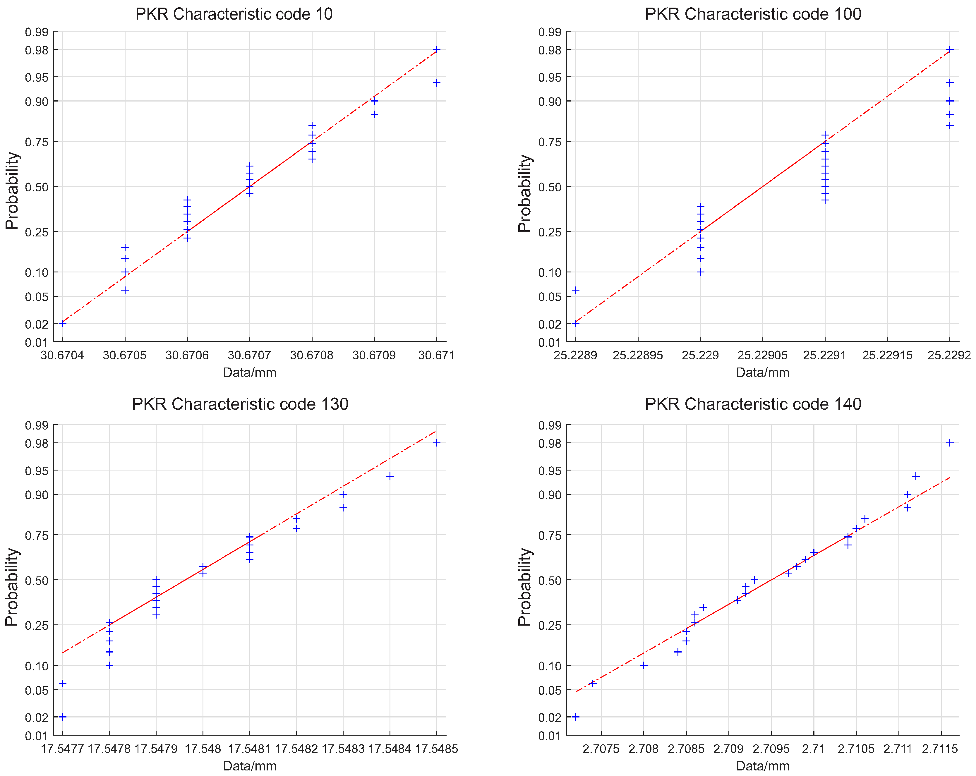
. Additionally, Figure 6 shows the normal probability plot, respectively, of characteristic codes 20 and 30 for a Magnet object, and Figure 7 shows the normal probability plot, respectively, of characteristic codes 10, 100, 130, and 140 for PKR object.

The normal distribution of the measured data allows the use of the capability index $C_p$.

Results provide the first selected graphs for the Magnet object. The following are selected graphs for the PKR object. For each repetition of the scenario, an MSA type-1 analysis was performed for each characteristic code. The selected statistical characteristics obtained from the MSA study are the capability factor $C_p$, the range of measurements R, and $6\sigma$ (standard deviation) of the individual repetitions. The relationship between $C_p$ and $6\sigma$ is described in (2), and the range of measurements R has no mathematical relationship with the $C_p$ factor and $6\sigma$ but, in many cases, suggests a similar trend. Additionally, outliers, which are not seen on $\sigma$, can be seen on the R graphs.

4.1. Results for the Magnet object

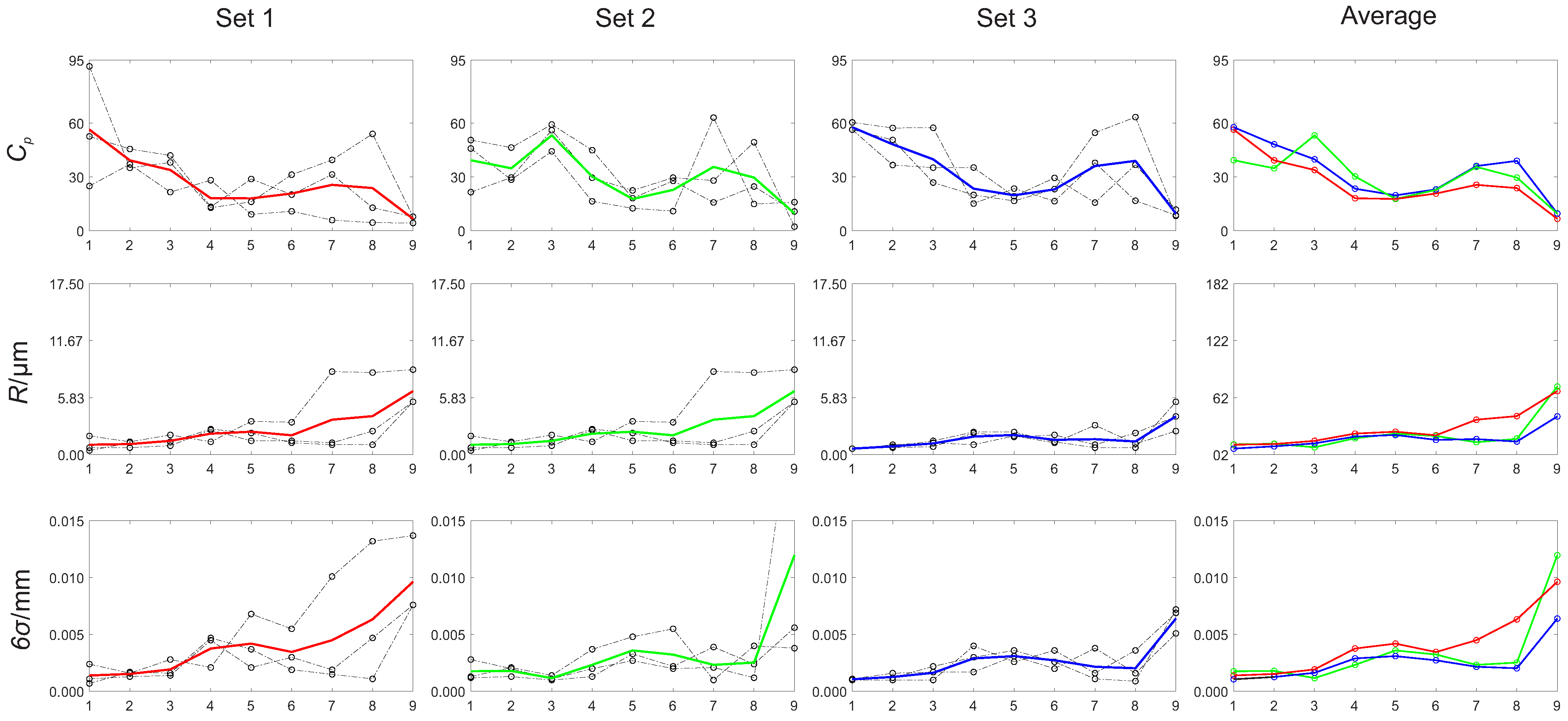
Figure 8 and Figure 9 present the measurement data calculated by the MSA type-1 analysis separately for the characteristic codes 20 and 30 for the object Magnet. The first row represents the capability factor $C_p$, the second row depicts the range of measurements R, and the third row shows the $6\sigma$ values. The columns represent the individual measurement sets: the first column measurement set 1, the second column measurement set 2, and the third column measurement set 3. In contrast, the last column shows only the average values of the individual sets on a common graph. The red color represents the average values of set 1, the green color represents the average values of set 2, and the blue color represents the average measurements of set 3. The black dotted lines represent individual repetitions of a particular set of measurements. The absolute value of statistical parameters ($C_p$, R, and $6\sigma$) is not as significant as the decreasing/increasing trend.

4.2. Results for the PKR Object

Figure 10 shows the measurement data calculated for the MSA type-1 analysis for the characteristic codes 10, 100, 130 and 140 for the object PKR. The first row represents the capability factor $C_p$, the second row shows the range of measurements R, and the third row shows the $6\sigma$ values. The first column represents the measurements of the characteristic code 10, the second column represents the measurements of the characteristic code 100, the third column represents the measurements of the characteristic code 130, and the fourth column represents the measurements of the characteristic code 140. The red, green, and blue lines represent the individual measurements, while the black lines represent the average measurement values. The absolute value of statistical parameters ($C_p$, R, and $6\sigma$) is not as significant as the decreasing/increasing trend.

5. Discussion

It should be underlined that the primary goal of our research was not to confirm the ability of the measuring system but to investigate the influence of various robot interventions made with the measured object on the final dimensional measurements. In automated measurements in industry, it is assumed that the measurement uncertainty is much lower than in traditional, manual measurement methods. The main reason for this assumption is human/operator influence on measurements. In the case of automated measurements, this influential factor is typically reduced or eliminated.

As can be seen from a general observation of Figure 8, Figure 9 and Figure 10, the robot actions do influence the dimensional measurements. Furthermore, various robot interventions do not have the same impact on the measurement capability of the measurement system. While observing more closely, Figure 8, Figure 9 and Figure 10 in comparison to Figure 3 and Figure 4, that describe the measurement codes, it turns out that the influence is noticeable in the length measurements (Magnet code 30, PKR codes 10, 100, and 140), while, in the spherical geometries, the influence is less recognizable (Magnet code 20 and PKR code 130).

The results describing the measurement results obtained from the MSA study for the Magnet characteristic code 20 (diameter) are shown in Figure 8. Increasing the degree of the robot’s manipulation (moving from scenario 1 to scenario 9) does not influence the dimensional measurements. The $C_p$, R, and $6\sigma$ values do not change significantly from scenario 1 to scenario 9. Furthermore, their values remain similar for all three measurement sets, representing the different measurement methods (last column). Measurement set 1 consists of measurements with the Touch-trigger-based measurement method (red line), set 2 consists of measurements with SM (green line) and an increased number of sampling points, and set 3 consists of measurements with SM+, with an additionally increased number of sampling points (blue line). The black dotted lines represent repetitions of a particular measurement method for all the scenarios.

As is clear from Figure 9, which represents the measurement results for the Magnet characteristic code 30 (height), various robot interventions influence the dimensional measurements. By increasing the degree of manipulation, the $C_p$ value decreases and the values R and $6\sigma$ increase from scenario 1 to scenario 9. Similar to the measurements of the Magnet characteristic code 20 are the curves describing $C_p$, R, and $6\sigma$ for the Magnet code 30 for all three measurement sets corresponding to three measurement methods (Figure 9, last column). In all three cases, the $C_p$ value decreases with an increase of the robot’s degree of manipulation, which means an increase in the scatter of the measurement data ($6\sigma$).

The Magnet object was our primary case study investigating the influence of robot manipulation on dimensional measurements in rectangular and spherical geometries. For this reason, more measuring sets were collected for the Magnet object than for the PKR object. The importance of the PKR object is that there are more added measurement codes. Furthermore, it served for the verification of the previously observed trends. The measurements on the PKR object confirmed the findings of the robot’s manipulation influence on the dimensional measurements obtained with the Magnet object.

Figure 10 shows measurements for the PKR object characteristic codes 10, 100, 130, and 140. The characteristic codes 10, 100, and 140 represent length measurements, and, by increasing the robot’s degree of manipulation, the trend of the decrease of the $C_p$ value and the increase of R and $6\sigma$ can be observed for all three cases. In the case of the PKR object characteristic code 130, which represents the spherical geometry, a decrease of the $C_p$ value is present but, in comparison with the other codes, to a much lesser extent. The R and $6\sigma$ values, in this case, do not increase significantly.

The similarity between the measurement results for the different measurement methods is not surprising. A comparable measurement uncertainty for TTM and SM was shown by Bastas [12] for rectangular and spherical geometries. They also showed that the measurement uncertainty decreases with an increasing number of sampling points. In our case, we could not prove a direct relationship between the number of sampling points and the factor $C_p$, as the differences between the measurement sets, which have different numbers of sampling points, were practically negligible. From a statistical point of view, the measurement methods TTM and SM are equivalent, so, from the process measurements’ point of view, SM is more desirable, as it enables shorter measurement cycles.

Due to the Equator measurement device’s comparative measurement principle, the absolute ambient temperature did not play a significant role. However, variations do play a more critical role. If the ambient temperature changes by more than the allowed temperature deviation, it is necessary to perform a re-master procedure, which “re-calibrates” the Equator. A direct relationship between the measurement uncertainty and the magnitude of the change in the ambient temperature was shown by Papananias et al. in Reference [21]. It turns out that, with a larger allowable temperature deviation between individual measurements, the measurement uncertainty increases exponentially and decreases with the implementation of the re-master procedure for relatively small temperature changes. The allowable temperature range in our study was defined as $T_a=T_m\pm 1^{\circ }$, where $T_m$ is the ambient temperature during the master procedure. Observing individual repetitions within the measurement sets, it can be argued that the ambient temperature was stable, since none of the repetitions triggered a request to perform a re-master procedure.

By comparing Set 1, Set 2, and Set 3 (TTM, SM, and SM+) in Figure 8, as well as in Figure 9, it can be confirmed that different measurement methods and the number of sampling points do not play a significant role in the final dimensional measurements. Based on the used comparative method with frequent re-mastering, it can be stated that the ambient temperature and variation of it also have a minimal impact.

Angular misalignment could be the reason for the increase of the $6\sigma$ and R values and the consequent decrease in the value of the factor $C_p$. The positional misalignment was not noticeable. This would happen by increasing the degree of the robot’s manipulation. An angular misalignment represents the misalignment of the measurement object’s orientation in the fixture between measurements compared to the object’s orientation in the fixture during the re-master procedure. The misalignment error is manifested as a loose fit of the subjects in the pallet, in the re-gripping position and the fixture, as well. Increasing the degree of the robot’s manipulation means more manipulation or more extended robot movements, and above all, an increase in the number of gripping sequences during the measurement process. For example, scenario 1 does not involve any gripping sequence, which means the misalignment error is practically zero. With the added short gripping sequence in scenario 2, a small amount of misalignment error is already present. As evident from Figure 9 and Figure 10, in the case of length measurements (Magnet code 30 and PKR codes 10, 100, and 140), the misalignment error increases with an increase in the degree of robot manipulation, resulting in a decrease of the $C_p$ value.

The cause is also in the axially symmetrical shape of both objects, Magnet and PKR. Due to the axial symmetry, there is no pronounced edge that would easily ensure optimal rotation of the object in the gripper and, consequently, at the Equator’s measuring point. Because of the robot’s repeatability and accuracy errors, and due to the overall gripping situation, one of the fingers comes into contact with the object earlier than the other and not entirely in the intended place, which, combined with the loose fit, result in a small, but unwanted, rotation. A tighter fit would be a potential solution. However, we must be aware of the limitations of tightness. A tight fit requires a very accurate and tight object positioning in the fixture. In the case of a too tight fixation of the object in the pallet (or fixture), the robot with the gripper will not be able to pick the object out of a particular place (the object would slip from the grip). A similar situation applies to the placement of the object. An excessive gripper force would also cause damage or deformation to the subject.

The most significant impact on angular misalignment originates from grasping and tightness in fit to fixture. Further, robot positional and orientational errors increase object-to-fixture interaction forces and, this way, cause increased misalignment.

It is evident that a higher number of grasps of the measured object with a robotic gripper causes a greater scatter of the measurements (scenarios 8 and 9). The same applies to the number of active joints of the robot when performing movements. A lower number of active joints (scenarios 3 and 4) during robot movements means minor scatter of measurement data than movements with a higher number of active joints. Nevertheless, minor changes in the object’s orientation also result in less scatter. Practical suggestions originating from this work are minimization of grasping actions, minimization of active joints, and manipulation and measurement sequence optimization.

For measurements with the Equator, special fixtures were developed to position objects with a robot in the Equator’s working area. Fixtures were designed to fit the object’s inner diameter, while the spring provides an additional tight fit, as shown in Figure 5. The $C_p$ values for scenarios 1 for all the measurement sets show that the fixtures are suitable for the given characteristics. Furthermore, it is clear that the whole measuring system (robot, fixture, Equator, and other peripherals) is capable in every scenario for all the characteristics of achieving the minimum calculated values of the $C_p$ factor, which were, respectively, 7.3, 2.3, 2.6, 3.1, 7.4, 30.1, and 3.0, for the Magnet characteristics 20 and 30 and PKR characteristics 10, 100, 130, and 140. In the most common cases, the minimum allowable $C_p$ value is set as $C_{p,min}=1.33$. In the worst case, the calculated capability factor $C_p$ of the measurement system is approximately twice as large ($C_p=2.3$ for Magnet code 20).

6. Conclusions

Product-quality and process control are gaining influence in the process industry and are an inherent part of Industry 4.0. Due to the increasing daily demands for product quality, the need for ever-improving measuring systems is also growing. In addition, the trend for automated measurements has been present for some time due to the improved reliability of the measurement results compared to the current traditional, manual measurements.

The main reason for measurement automation is the reduction or elimination of human-operator influence on the measurements.

Our research wanted to show that just as the operator impacts on the dimensional measurements, so does the robot manipulation. We divided the robot’s tasks into the functions of grip, rotation, translation, etc., which were the basis for the composition of nine different robot scenarios. The robot was used for serving the Equator measuring device.

This study recognized that the effect of the robot’s manipulation influence is much more pronounced for length measurements than for spherical geometries. Different measuring methods (TTM and SM, different number of sampling points) were used, which showed similar trends in the measurement data. The independence of using different measurement methods on the final dimensional measurements directly indicates the influence of robot manipulation.

The main influential factor for decreasing the capability factor $C_p$ with an increased degree of robot manipulation was an angular misalignment of the measured part compared to the master part in the re-master procedure. Angular misalignment is manifested as a set of errors due to the robot’s inaccuracy and repeatability errors, the loose fit of the measured object in the pallet and the intermediate mechanical fixture (re-gripping), and the error in the gripping phase. The following steps would investigate the impact of the gripping error compared to the robot’s accuracy and repeatability.