Hybrid NHPSO-JTVAC-SVM Model to Predict Production Lead Time

Abstract

In the shipbuilding industry, each production process has a respective lead time; that is, the duration between start and finish times. Lead time is necessary for high-efficiency production planning and systematic production management. Therefore, lead time must be accurate. However, the traditional method of lead time management is not scientific because it only references past records. This paper proposes a new self-organizing hierarchical particle swarm algorithm (PSO) with jumping time-varying acceleration coefficients (NHPSO-JTVAC)-support vector machine (SVM) regression model to increase the accuracy of lead-time prediction by combining the advanced PSO and SVM models. Moreover, this paper compares the prediction results of each SVM-based model with those of other conventional machine-learning algorithms. The results demonstrate that the proposed NHPSO-JTVAC-SVM model can achieve further meaningful enhancements in terms of prediction accuracy. The prediction performance of the NHPSO-JTVAC-SVM model is also better than that of the other SVM-based models or other machine learning algorithms. Overall, the NHPSO–JTVAC-SVM model is feasible for predicting the lead time in shipbuilding.

1. Introduction

In the shipbuilding industry, an essential part of scientific management is lead time, which is necessary for shipyards to arrange production plans, particularly in production organization and progress of production control [1,2]. Additionally, lead time is closely related to the production efficiency of frontline manufacturing workers. The rationality of its arrangement directly affects workers’ production enthusiasm, thereby affecting product quality and labor productivity [3]. For example, if the evaluation of lead time is insufficient and management has not prepared the appropriate plan for construction peaks, the construction cycle will be prolonged. Here, to avoid affecting the construction cycle, workers must operate overtime for long periods, resulting in a decline in construction quality. Conversely, if the evaluation of lead time is overestimated, it results in excess construction capacity problems and human resource waste [4]. Consequently, lead time should be arranged reasonably, which means that the planned lead time must be as close as possible to the actual lead time in the shipyards’ production planning stage. However, because the shipbuilding industry is a labor-intensive industry, this has resulted in a significant difference between planned and actual lead times (Figure 1). Therefore, to rationalize the lead time arrangement, lead-time prediction becomes particularly critical [2,4,5].

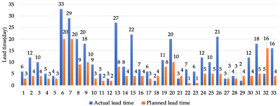
Figure 1. Differences in planned and actual lead times.

For many years, managers frequently used the experience evaluation method to specify lead time [6]. However, this method is time-consuming and inefficient. Thus, production planning and scheduling (PPS) cannot be properly organized, making shipyard management ineffective [7]. Lead time is affected by various factors and restricted by various conditions [8]. Several researchers have studied the lead time of production, and some results have been achieved [7,9,10].

In recent research, machine learning (ML) has been widely applied in the prediction of production lead time to understand the complex relationship between lead time and its affecting factors. Gyulai et al. [9] proposed using ML algorithms to predict the lead time of jobs in the manufacturing flow-shop environment; the results indicated that ML algorithms can sufficiently understand the non-linear relationship, and they obtained good prediction accuracy from ML models. Lingitz et al. [7] analyzed the key features of lead time, provided importance scores, and developed ML models to predict lead time in the semiconductor manufacturing industry. In particular, Jeong et al. [10] attempted to improve production management capabilities by analyzing the lead time based on spool fabrication and painting datasets. They applied ML algorithms and compared the performance of each.

In ML, the SVM algorithm, proposed by Vapnik [11] in 1995, is widely used in the prediction field. Because it is based on statistical learning theory and the principle of structural risk minimization, an SVM can theoretically converge on the global optimal solution of a problem. Moreover, it exhibits unique advantages in solving small samples and nonlinear problems. It has strong generalization ability and has become a popular research topic in the field of industrial forecasting. Thissen et al. [12] applied an SVM model to predict time series. They demonstrated that the SVM model performs well in time-series forecasting. Zhang et al. [13] proposed using an SVM model to forecast the short-term load of an electric power system. They demonstrated that the forecast performance of the SVM model was better than that of a back-propagation neural network (BPNN). Astudillo et al. [14] used an SVM model to predict copper prices. The results indicated that the SVM model can predict copper-price volatilities near reality.

However, the disadvantage of an SVM is that it is too sensitive to parameters, and an efficient SVM model can be built only after its parameters are carefully selected [15]. Therefore, many researchers have proposed methods for optimizing SVM parameters (Table 1). For instance, Yu et al. [16] combined an SVM model with a PSO algorithm to predict man-hours in aircraft assembly. The forecasting results indicated that the PSO-SVM model was significantly better than the BPNN model. Wan et al. [17] suggested applying the PSO-SVM hybrid model to predict the risk of the expressway project. The prediction results showed that the proposed model was more accurate and better than the traditional SVM model. Lv et al. [18] used PSO-SVM, grid search (GS)-SVM models to predict steel corrosion. Compared with the GS-SVM model, the results showed that the PSO-SVM steel corrosion prediction model was more accurate. Additionally, Luo et al. [19] proposed the use of a genetic algorithm (GA) to optimize an SVM model. The overall results indicated that the GA is an excellent optimization algorithm for increasing the prediction accuracy of an SVM. In the landslide groundwater levels prediction field, the GA-SVM model was proposed by Cao et al. [20]. The results showed that the GA-SVM model can understand the relationship between groundwater level fluctuations and influencing factors well. Moreover, other researchers combined other meta-heuristic algorithms such as the bat algorithm (BA) and the grasshopper optimization algorithm (GOA) with SVMs, and obtained good results [21,22]. Unlike other studies, this paper proposes the application of a new self-organizing hierarchical PSO with jumping time-varying acceleration coefficients (NHPSO-JTVAC) algorithm, an advanced version of the PSO algorithm, to optimize the parameters in an SVM. Moreover, the NHPSO-JTVAC-SVM model is proposed to predict the lead time in the shipyard’s block assembly and pre-outfitting processes.

Table 1. Research literature on SVM optimization techniques.

	SVM Optimization Techniques	Prediction Field
Yu et al. [17]	PSO	1. Man-hours in aircraft assembly
Wan et al. [18]		2. Risk of the expressway project
Lv et al. [19]		3. Steel corrosion
Luo et al. [20]	GA	1. Vertical load capacity of driven piles in cohesionless soils
Cao et al. [21]		2. Landslide groundwater levels
Tavakkoli et al. [22]	BA	Printed circuit board sales
Barman et al. [23]	GOA	Short-term load
This paper	NHPSO–JTVAC	Lead time in shipyard’s process

The remainder of this paper is organized as follows: Section 2 introduces the algorithm principle of the hybrid predictive model. Section 3 describes the construction of the model. Section 4 discusses the experimental results, and Section 5 summarizes and concludes the paper.

2. Prediction Model

2.1. SVM

For non-linear regression problems, assume the training data $\left\{\left(x_1,y_1\right),\left(x_2,y_2\right),\cdots \left(x_i,y_i\right)\right\}, i=1, 2, \dots ,n, x_i\subset R^n, y_i\subset R$, where $n$ is the total number of training samples. The regression concept of SVM is to determine a non-linear mapping from the input to output and map the data to a high-dimensional feature space, in which the training samples can be regressed through a regression equation $f\left(x\right)$, where$f\left(x\right)$ can be expressed as the following equation [23]:

$$f\left(x\right)=\omega \cdot \phi \left(x\right)+b$$

(1)

where $w$ represents the weight vector, and $b$ represents the bias vector.

The SVM problem can be described as solving the following problem [24,25]:

$$\mathbf{minimize:}\frac{1}{2}{\Vert \omega \Vert }^2+C\sum _{i=1}^n\left({\xi }_i+{\xi }_i^{*}\right)$$

(2)

$$\mathbf{subject\; to:}\begin{array}{c}{y}_{i }-\left(\omega \cdot \phi \left(x_{i }\right)\right)-b\le \epsilon +{\xi }_i\\ \left(\omega \cdot \phi \left(x_{i }\right)\right)+b-y_{i }\le \epsilon +{\xi }_i^{*}\\ {\xi }_i,{\xi }_i^{*}\ge 0, i=1,2,3\dots n.\end{array}$$

(3)

where $C$ is the penalty parameter; ${\xi }_i \mathrm{and} {\xi }_i^{*}$ are the slack variables; $\epsilon$ is defined as the tube width; the $\epsilon$-insensitive loss function that controls the regression error is defined by the following formula [26]:

$$\begin{array}{cc}{L}_{\epsilon }\left(y_i,f(x_i)\right)=& \begin{array}{cc}\left|y_i-f\left(x_i\right)\right|-\epsilon ,for \left|y_i-f\left(x_i\right)\right|\ge \epsilon & \left(4\right)\\ 0, otherwise& \left(5\right)\end{array}\end{array}$$

Next, the SVM problem can be transformed into a dual-optimization problem [27]:

$$\mathbf{maximize:}-\frac{1}{2}{\displaystyle \sum }_{i,j=1}^n\left({\alpha }_i-{\alpha }_i^{*}\right)({\alpha }_j-{\alpha }_j^{*})K\left(x_i, x_j\right)-\epsilon {\displaystyle \sum }_{i=1}^n\left({\alpha }_i+{\alpha }_i^{*}\right)+{\displaystyle \sum }_{i=1}^n{y}_i\left({\alpha }_i-{\alpha }_i^{*}\right)$$

(6)

$$\mathbf{subject\; to:}\begin{array}{c}{\displaystyle {\displaystyle \sum }_{i=1}^n}\left({\alpha }_i-{\alpha }_i^{*}\right)=0, 0\le {\alpha }_i^{*}\le C,\\ i=1,2,3\dots n.\end{array}$$

(7)

Finally, the SVM regression function can be obtained from the following equation [28]:

$$f\left(x\right)={\displaystyle {\displaystyle \sum }_{i=1}^n}\left({\alpha }_i-{\alpha }_i^{*}\right)K\left(x_i,x\right)+b$$

(8)

where $K\left(x_i,x\right)$ is the kernel function of the SVM model. According to experience, when solving complex high-dimensional sample problems, the radial basis function (RBF, Equation (9)) kernel is better than other kernel functions. Therefore, the RBF is used as the kernel function in this study [29].

$$K\left(x_i,x\right)=exp\left\{-\Vert x_i-x{\Vert }^2/2{\sigma }^2\right\}$$

(9)

As shown above, the three most important parameters ($C$, $\epsilon$, $\sigma$) of the SVM nonlinear regression function must be determined by the user. Selecting appropriate values is challenging. To solve this problem, the optimization algorithm is described below.

2.2. NHPSO-JTVAC: An Advanced Version of PSO

2.2.1. PSO Algorithm

In 1995, inspired by the flocking behavior of birds, the PSO algorithm was introduced and developed by Kennedy and Eberhart [30]. This is a search algorithm used to solve optimization problems in computational mathematics. It is also one of the most classic swarm intelligent algorithms because of its fast convergence and simple implementation [31].

The PSO algorithm is conducted by first initializing a group of random particles and then determining the optimal solution through iteration. In each iteration, the particles track two extreme values to update themselves: the personal best (p-best) and global best (g-best) values. Each particle updates its speed and position according to the above two extreme values. If, in a D-dimensional target search space, the population number is $m$, where the position of the i-th particle in the d-th dimension is $x_{i,d}$, its velocity can be defined as $v_{i,d}$, the current p-best position of the particle is $p_{i,d}$, and the current g-best position of the entire particle swarm is $p_{g,d}$. Each particle’s velocity and position are updated according to the following formulations [32]:

$$v_{i,d}^{Iter+1}=\omega \times v_{i,d}^{Iter}+c_1^{Iter}\times r_{1,d}\times \left(p_{i,d}^{Iter}-x_{i,d}^{Iter}\right)+c_2^{Iter}\times r_{2,d}\times \left(p_{g,d}^{Iter}-x_{i,d}^{Iter}\right)$$

(10)

$$x_i^{Iter+1}=x_i^{Iter}+ v_i^{Iter+1}$$

(11)

where $i=1,2,3,\cdots ,m,d=1,2,3,\cdots ,D; r_1$ and $r_2$ are random numbers following the uniform (0, 1) distribution; $c_1$ and $c_2$ are learning factors; $\omega$ is the inertia weight that controls the current velocity of the particle, and its value is non-negative. The larger the value of ω, the greater the particle’s velocity, and the particle will perform a global search with a more significant step size; for smaller values of ω, the particle tends to perform a more finely local search. To balance global and local search capabilities, $\omega$ generally assumes a dynamic value. In addition, the linearly decreasing inertia weight (LDIW) strategy is most commonly used to determine the values of $\omega$ [33].

$$\omega ={\omega }_{max}-\left({\omega }_{max}-{\omega }_{min}\right)\times \frac{It\mathrm{e}r}{It\mathrm{e}{r}_{max}}$$

(12)

where $It\mathrm{e}r$ is the current number of iterations, $It\mathrm{e}{r}_{max}$ is the maximum number of iterations, and ${\omega }_{max}$ and ${\omega }_{min}$ are maximal/minimal inertia weights, frequently set to 0.9 and 0.4, respectively [34].

2.2.2. NHPSO-JTVAC Algorithm

The PSO algorithm has a fast convergence speed, but it sometimes falls into a local optimum, and there is no guarantee that it can search for the optimal solution [34].

To solve the above problems, HPSO-TVAC was proposed by Ratnaweera et al. [35] as an efficient improved algorithm of the classic PSO algorithm. Ghasemi et al. [36] proposed an enhanced version of HPSO-TVAC called NHPSO-JTVAC, which has better performance than the original HPSO-TVAC algorithm. To avoid particles falling into local optima, they are afforded the ability to suddenly jump out during the algorithm iteration according to Equations (13)–(15):

$$c^{Iter}=\left(c_f-c_i\right)\times \frac{It\mathrm{e}r}{It\mathrm{e}{r}_{max}}+c_i$$

(13)

$$c_1^{Iter}={\left|w\right|}^{\left(c^{Iter}\times w\right)}$$

(14)

$$c_2^{Iter}={\left|1-w\right|}^{(c^{Iter}/\left(1-w\right))}$$

(15)

where $c^{Iter}$ changes from $c^1=c_i=0.5$to $c^{It\mathrm{e}{r}_{max}}=c_f=0$, and $w$ is defined as a standard normal random value. Unlike Equation (10), the new search equation is given as:

$$\begin{array}{c} v_{i,d}^{Iter+1}=c_1^{Iter}\times r_{1,d}\times \left(p_{i,d}^{Iter}-x_{i,d}^{Iter}\right)+c_2^{Iter}\times r_{2,d}\\ \times \left(\left(p_{g,d}^{Iter}+p_{r,d}^{Iter}\right)-2\times x_{i,d}^{Iter}\right)\end{array}$$

(16)

where $p_{r,d}^{Iter}$ represent the best personal solution of a randomly selected particle (such as the r-th particle).

2.3. Applying NHPSO-JTVAC to SVM

To select the appropriate parameters for an SVM, the NHPSO-JTVAC algorithm proposed in Section 2.2.2 was applied to optimize the parameters of the SVM. Figure 2 illustrates the SVM flow chart based on the NHPSO-JTVAC algorithm.

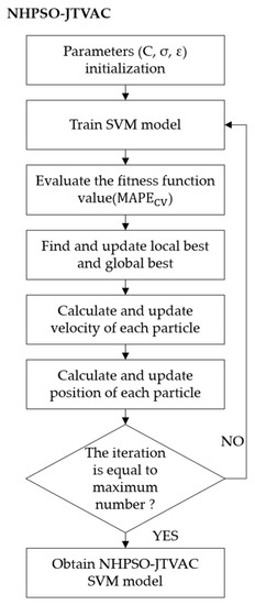
Figure 2. Flow chart of SVM based on NHPSO-JTVAC.

• Preprocess the data, and then split the dataset randomly into a training and test set (8:2).
• Randomly initialize the velocity and position of the particles, where the position vector (3-dimensional) represents the three parameters ($C$, $\epsilon$, $\sigma$) of the SVM.
• Calculate the fitness value of each particle and determine the current p-best and g-best positions. The fitness function selected in this study was the mean absolute percentage error (MAPE) function (Equation (17)). Figure 3 illustrates the concept of k-fold cross-validation (CV). To prevent the model from overfitting, a 5-fold CV method was adopted in this study [37].

  $$fitness\left(MAP{E}_{CV}\right)=\frac{100\%}{m}{\displaystyle \sum }_{i=1}^m\left|\frac{y_i-{\widehat{y}}_i}{y_i}\right|$$

  (17)

  where$m$ is the number of training samples, $y_i$ is the actual value, and ${\widehat{y}}_i$ is the predicted value.
  

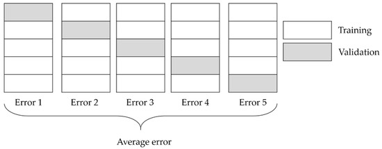  Figure 3. Concept of k-fold cross-validation (k = 5).
• For each particle, compare its fitness value with the p-best position it has experienced. If this is better, use it as the current p-best position.
• For each particle, compare its fitness value with the g-best position. If this is better, replace its fitness value with the g-best.
• Calculate and update the velocity and position of each particle.
• If the termination condition is not satisfied, return (b); otherwise, the optimal solution is obtained, and the algorithm ends.

3. Lead-Time Prediction Based on NHPSO-JTVAC-SVM

3.1. Data and Preparation

This paper presents a hybrid artificial intelligence (AI) model to predict the lead time in the shipyard block process. As shown in Table 2, we applied it to two datasets collected from a shipyard’s block assembly and a pre-outfitting process to evaluate the proposed model. The assembly and pre-outfitting processes consisted of information from 4779 and 4198 blocks. Each dataset was split into training and test data. Eighty percent of each dataset, 3823 and 3358 data points, was used to train data individually, and 20% of each dataset, 956 and 840 data points, was used to test data separately.

Table 2. Data collection.

No.	Dataset	Prediction Target
1	Assembly process performance data	Lead time
2	Pre-outfitting process performance data	Lead time

The target value (label) of each dataset was the lead time. A part of the original dataset is shown in Figure 4a,b.

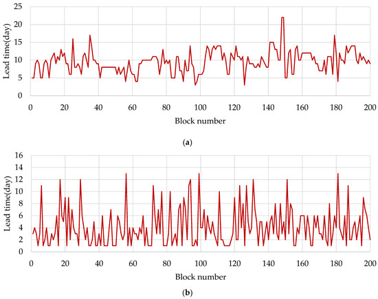
Figure 4. Original dataset of (a) block assembly process and (b) block pre-outfitting process.

3.1.1. Data Normalization

To eliminate the effect of significant differences between the different scales on the learning speed, prediction accuracy, and generalizability of the SVM, we performed normalization preprocessing on the training and test samples, and the data were normalized to [0, 1]. The normalization formula was as follows:

$$x_{scaled}=\frac{x-x_{m_{in}}}{x_{m_{ax}}-x_{m_{in}} }$$

(18)

3.1.2. Feature Selection

Feature selection (FS) of the machine learning model is essential. FS avoids the data dimensions problem and reduces learning difficulty. We performed feature engineering and removed irrelevant features.

As shown in Figure 5, the FS steps were as follows:

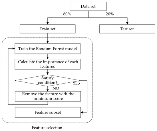
Figure 5. Flow chart of feature selection.

Step 1.

The data are split into the training and test sets (8:2).

Step 2.

The random forest (RF) model is trained using a training set.

Step 3.

The importance score for each feature in the training set is calculated. Features are ranked by feature importance scores.

Step 4.

Suppose the model’s accuracy and execution time are not satisfied. In that case, the feature with the minimum importance score will be deleted from the data set, and Steps 2 and 3 will be repeated until the desired number of features is obtained. Otherwise, the feature subset is obtained directly.

3.1.3. Parameter Setting

As shown in Figure 6, for comparison with the proposed algorithm NHPSO-JTVAC, we also applied other meta-heuristic algorithms such as PSO, BA, GA, and GOA [38,39,40,41] and compared the performance of each algorithm with the others.

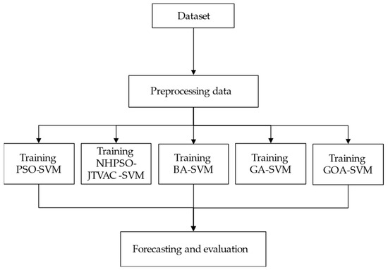
Figure 6. Flow chart of the prediction models.

In all the algorithms, the population size was unified and set to 20, and the number of iterations set to 500. The search space dimension of each algorithm was set to 3, which represented the three parameters ($C$, $\epsilon$, $\sigma$) of the SVM. The search range of $C$ was set to [${10}^0$, ${10}^3$], $\epsilon$ was set to [${10}^{-3}$,${10}^0$], and $\sigma$ was set to [${10}^{-2}$,${10}^1$]. The remaining parameters of the NHPSO-JTVAC were set as listed in Table 3. Furthermore, the initial parameters of PSO, GA, BA, and GOA were set as listed in Appendix A (Table A1).

Table 3. Parameter setting of the NHPSO-JTVAC algorithm.

NHPSO-JTVAC []	Parameter Setting
Number of particles	20
Number of search dimensions	3
Range of SVM parameters	$C$[${10}^0$, ${10}^3$]
	$\epsilon$[${10}^{-3}$,${10}^0$]
	$\sigma$[${10}^{-2}$,${10}^1$]
$c^{Iter}$	Changing from $c^1=c_i=$0.5 to $c^{It\mathrm{e}{r}_{max}}=c_f=$ 0
Maximum number of generations	500

3.1.4. Performance Metrics

To measure prediction accuracy, this study applied certain widely used regression prediction performance metrics: root-mean-square error (RMSE), mean absolute error (MAE), and MAPE, as shown in Table 4. Here, $N$ is the sample size, $y_i$ is the actual value, and ${\widehat{y}}_i$ is the predicted value.

Table 4. Regression prediction performance metrics.

Metrics	Calculation
RMSE $\left(y,\widehat{y}\right)$	$\sqrt{\frac{1}{N}{\displaystyle {\displaystyle \sum }_{i=1}^N}{\left(y_i-{\widehat{y}}_i\right)}^2}$
MAE $\left(y,\widehat{y}\right)$	$\frac{1}{N}{\displaystyle {\displaystyle \sum }_{i=1}^N}\left|y_i-{\widehat{y}}_i\right|$
MAPE $\left(y,\widehat{y}\right)$	$\frac{100\%}{N}{\displaystyle {\displaystyle \sum }_{i=1}^N}\left|\frac{y_i-{\widehat{y}}_i}{y_i}\right|$

Lower values of MAPE, MAE, and RMSE indicate higher accuracy of the model, meaning that the prediction results are more convincing. According to the MAPE metric, which has been widely applied to evaluate industrial and business data, when MAPE < 10%, it can be considered as highly accurate forecasting; when 10% < MAPE < 20%, it can be considered as good forecasting; when 20% < MAPE < 50%, we can see it as reasonable forecasting; when MAPE >50%, the interpretation is inaccurate forecasting [42].

4. Experimental Results

We conducted prediction experiments using test data to verify the proposed NHPSO-JTVAC-SVM model. We compared the model with SVM, NHPSO-JTVAC-SVM, BA-SVM, GA-SVM, and GOA-SVM. The 5-fold CV scores in the iterative process of the integrated models are shown graphically in Figure 7a,b. The best 5-fold CV scores searched by the five models are listed in Table 5. The results demonstrated that the NHPSO-JTVAC algorithm had the best search performance with the best fitness values of 12.92% and 20.19% in the block assembly process performance dataset and pre-outfitting process performance dataset, respectively.

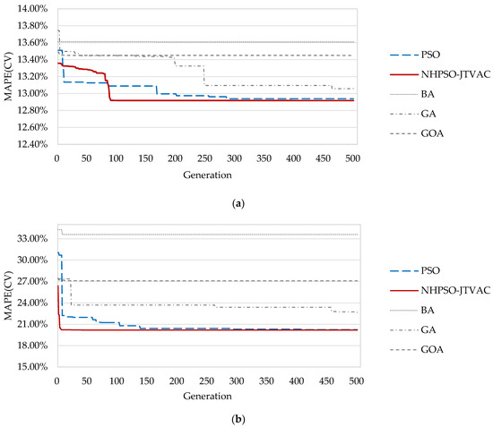
Figure 7. Generation of the optimization models in (a) block assembly process performance dataset and (b) block pre-outfitting process performance dataset.

Table 5. K-fold CV scores (MAPE) of each model.

Dataset		SVM	PSO-SVM	NHPSO-JTVAC-SVM	BA-SVM	GA-SVM	GOA-SVM
Assembly process performance data	Kfold_1	13.71%	13.26%	13.24%	14.01%	13.42%	13.68%
	Kfold_2	13.96%	12.46%	12.44%	13.25%	12.61%	13.10%
	Kfold_3	14.07%	13.49%	13.45%	14.46%	13.63%	14.10%
	Kfold_4	13.27%	12.31%	12.31%	12.53%	12.30%	12.93%
	Kfold_5	14.08%	13.17%	13.14%	13.80%	13.32%	13.45%
	${\mathrm{MAPE}}_{\mathrm{CV}}$(Mean)	13.82%	12.94%	12.92%	13.61%	13.06%	13.45%
Pre-outfitting process performance data	Kfold_1	24.29%	20.60%	20.49%	34.42%	22.51%	28.15%
	Kfold_2	24.22%	20.98%	20.95%	32.55%	23.17%	27.64%
	Kfold_3	23.55%	20.28%	20.11%	35.04%	22.54%	26.21%
	Kfold_4	22.79%	19.71%	19.63%	34.93%	22.10%	26.66%
	Kfold_5	22.78%	19.65%	19.77%	31.10%	23.04%	26.77%
	${\mathrm{MAPE}}_{\mathrm{CV}}$(Mean)	23.53%	20.25%	20.19%	33.61%	22.67%	27.09%

Table 6 shows the optimal values of the three SVM parameters ($C$, $\epsilon$, and $\sigma$) for each SVM-based model. In addition, Table 7 shows the test accuracy of these models based on the MAE, RMSE, and MAPE. The test error of MAPE, which we set as the fitness function of the optimization process, is shown graphically in Figure 8. We observed that the NHPSO-JTVAC-SVM model had the smallest MAPE in the training set (5-fold CV) and the smallest error in the test set. The results indicated that the test errors of the NHPSO-JTVAC-SVM model were the smallest in these models. In the block assembly process performance dataset, the MAPE of the NHPSO-JTVAC-SVM algorithm was 11.79%, and the MAE was 0.89. Moreover, in the pre-outfitting process performance dataset, the MAPE and MAE were 17.86% and 0.96, respectively. In addition, the NHPSO-JTVAC-SVM model was significantly better than the SVM model.

Table 6. Optimal values of the three SVM parameters ($C$, $\epsilon$, and $\sigma$).

Model	Dataset	$C$	$\epsilon$	$\sigma$
PSO-SVM	Assembly process performance data	6.80	0.0172	6.8432
	Pre-outfitting process performance data	604.69	0.0157	0.0864
NHPSO-JTVAC-SVM	Assembly process performance data	5.87	0.0010	7.6115
	Pre-outfitting process performance data	997.94	0.0192	0.0666
BA-SVM	Assembly process performance data	113.65	0.1403	1.2904
	Pre-outfitting process performance data	201.55	0.3233	0.0509
GA-SVM	Assembly process performance data	13.03	0.0353	4.7538
	Pre-outfitting process performance data	228.40	0.0283	0.1842
GOA-SVM	Assembly process performance data	6.23	0.3650	6.3992
	Pre-outfitting process performance data	143.44	0.3556	0.0853

Table 7. Test errors of each model.

Dataset		SVM	PSO-SVM	NHPSO-JTVAC-SVM	BA-SVM	GA-SVM	GOA-SVM
Assembly process performance data	MAPE (%)	13.40	11.81	11.79	12.55	11.96	12.14
	MAE	0.99	0.89	0.89	0.95	0.90	0.91
	RMSE	1.25	1.23	1.23	1.29	1.25	1.18
Pre-outfitting process performance data	MAPE (%)	21.24	17.98	17.86	29.99	20.21	25.58
	MAE	1.05	0.96	0.96	1.29	0.97	1.09
	RMSE	1.95	1.91	1.91	2.19	1.86	1.92

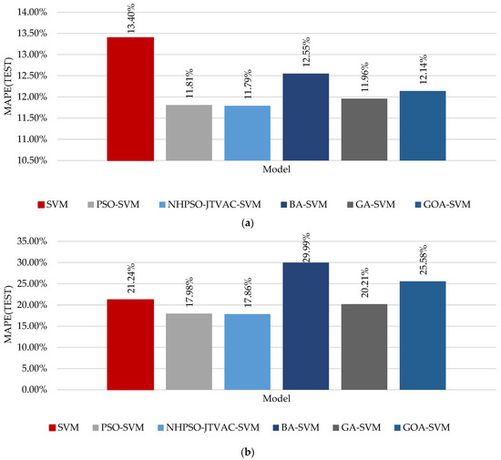
Figure 8. Test MAPE of each model in (a) block assembly process performance dataset and (b) block pre-outfitting process performance dataset.

Table 8 lists the average MAPE values based on two datasets and obtained using SVM, PSO-SVM, NHPSO-JTVAC-SVM, BA-SVM, GA-SVM, and GOA-SVM. The average MAPE for the NHPSO-JTVAC-SVM model was 14.83%, which was the smallest among the AI models. Furthermore, Figure 9 shows the predicted results of the test set for different datasets, wherein the NHPSO-JTVAC-SVM model was superior in solving the lead-time-prediction problems.

Table 8. Average MAPE of SVM, PSO-SVM, NHPSO-JTVAC-SVM, BA-SVM, GA-SVM, and GOA-SVM.

	SVM	PSO-SVM	NHPSO-JTVAC-SVM	BA-SVM	GA-SVM	GOA-SVM
MAPE (%)	17.32	14.90	14.83	21.27	16.09	18.86

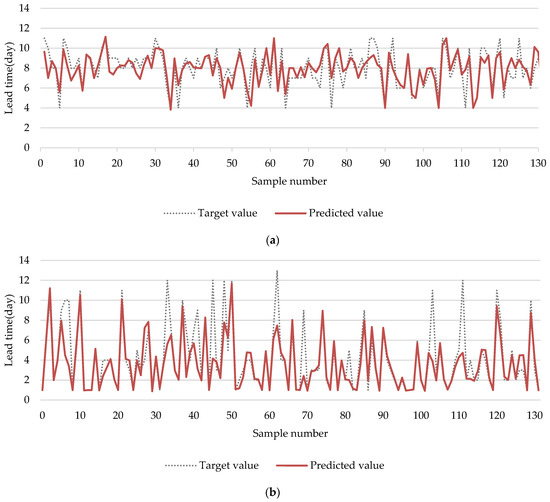
Figure 9. NHPSO-JTVAC-SVM model’s predicted results of the (a) block assembly process performance test set and (b) block pre-outfitting process performance test set.

Finally, we compared the proposed NHPSO-JTVAC-SVM model with other conventional ML models, such as the ElasticNet and adaptive boosting (AdaBoost) models. The results indicated that the NHPSO-JTVAC-SVM model we developed had the best performance (Table 9).

Table 9. Comparison with other machine models.

Scenario		ElasticNet	AdaBoost	NHPSO-JTVAC-SVM
Assembly process performance data	MAPE (%)	21.67	16.52	11.79
	MAE	1.50	1.16	0.89
	RMSE	1.85	1.43	1.23
Pre-outfitting process performance data	MAPE (%)	118.50	40.52	17.86
	MAE	2.63	1.49	0.96
	RMSE	3.23	2.07	1.91

5. Conclusions

Based on the analysis of the parameter performance of SVMs, this paper proposes a hybrid NHPSO-JTVAC-SVM lead-time-prediction model. It fully utilizes the global search feature of the NHPSO-JTVAC algorithm to optimize the parameters of an SVM, which overcomes the blindness of SVM parameter selection. Compared with commonly used methods, the parameter selection in this paper provides clearer theoretical guidance. Additionally, in the process of searching for parameters, the NHPSO-JTVAC algorithm is superior in terms of performance. Furthermore, the experimental results indicated that the NHPSO-JTVAC-SVM prediction model has good prediction accuracy. Overall, the results indicated that the optimized model is better than other machine learning models.

Note that the fitness function used in this study was the MAPE. Although the test error MAPE of the NHPSO-JTVAC model was better than other models, other performance metrics such as RMSE were worse than those of other models such as GOA-SVM and GA-SVM. To optimize the model further, we may develop an optimization algorithm that considers multi-fitness functions, an important aspect of future research.

References

- Tatsiopoulos, I.; Kingsman, B. Lead time management. Eur. J. Oper. Res. 1983, 14, 351–358. [Google Scholar] [CrossRef]
- Öztürk, A.; Kayalıgil, S.; Özdemirel, N.E. Manufacturing lead time estimation using data mining. Eur. J. Oper. Res. 2006, 173, 683–700. [Google Scholar] [CrossRef]
- Lee, J.; Peccei, R. Lean production and quality commitment. Pers. Rev. 2008, 37, 5–25. [Google Scholar] [CrossRef]
- Brown, S.D.; Khan, H.; Salley, R.S.; Zhu, W. Lead Time Estimation Using Artificial Intelligence; LMI Tysons Corner United States: Tysons, VA, USA, 2020. [Google Scholar]
- Sethi, F. Using Machine Learning Methods to Predict Order Lead Times. Int. J. Sci. Basic Appl. Res. 2020, 54, 87–96. [Google Scholar]
- Berlec, T.; Govekar, E.; Grum, J.; Potocnik, P.; Starbek, M. Predicting order lead times. Stroj. Vestn. 2008, 54, 308. [Google Scholar]
- Lingitz, L.; Gallina, V.; Ansari, F.; Gyulai, D.; Pfeiffer, A.; Sihn, W.; Monostori, L. Lead time prediction using machine learning algorithms: A case study by a semiconductor manufacturer. Procedia Cirp 2018, 72, 1051–1056. [Google Scholar] [CrossRef]
- Zijm, W.H.; Buitenhek, R. Capacity planning and lead time management. Int. J. Prod. Econ. 1996, 46, 165–179. [Google Scholar] [CrossRef][Green Version]
- Gyulai, D.; Pfeiffer, A.; Nick, G.; Gallina, V.; Sihn, W.; Monostori, L. Lead time prediction in a flow-shop environment with analytical and machine learning approaches. IFAC-PapersOnLine 2018, 51, 1029–1034. [Google Scholar] [CrossRef]
- Jeong, J.H.; Woo, J.H.; Park, J. Machine Learning Methodology for Management of Shipbuilding Master Data. Int. J. Nav. Archit. Ocean Eng. 2020, 12, 428–439. [Google Scholar] [CrossRef]
- Cortes, C.; Vapnik, V. Support-vector networks. Mach. Learn. 1995, 20, 273–297. [Google Scholar] [CrossRef]
- Thissen, U.; Van Brakel, R.; De Weijer, A.; Melssen, W.; Buydens, L. Using support vector machines for time series prediction. Chemom. Intell. Lab. Syst. 2003, 69, 35–49. [Google Scholar]
- Zhang, M.-G. Short-term load forecasting based on support vector machines regression. In Proceedings of the 2005 International Conference on Machine Learning and Cybernetics, Guangzhou, China, 18–21 August 2005; pp. 4310–4314. [Google Scholar]
- Astudillo, G.; Carrasco, R.; Fernández-Campusano, C.; Chacón, M. Copper Price Prediction Using Support Vector Regression Technique. Appl. Sci. 2020, 10, 6648. [Google Scholar] [CrossRef]
- Duan, K.; Keerthi, S.S.; Poo, A.N. Evaluation of simple performance measures for tuning SVM hyperparameters. Neurocomputing 2003, 51, 41–59. [Google Scholar] [CrossRef]
- Yu, T.; Cai, H. The prediction of the man-hour in aircraft assembly based on support vector machine particle swarm optimization. J. Aerosp. Technol. Manag. 2015, 7, 19–30. [Google Scholar] [CrossRef]
- Wan, A.; Fang, J. Risk Prediction of Expressway PPP Project Based on PSO-SVM Algorithm. In ICCREM 2020: Intelligent Construction and Sustainable Buildings; American Society of Civil Engineers: Reston, VA, USA, 2020; pp. 55–63. [Google Scholar]
- Lv, Y.-J.; Wang, J.-W.; Wang, J.J.-L.; Xiong, C.; Zou, L.; Li, L.; Li, D.-W. Steel corrosion prediction based on support vector machines. Chaos Solitons Fractals 2020, 136, 109807. [Google Scholar] [CrossRef]
- Luo, Z.; Hasanipanah, M.; Amnieh, H.B.; Brindhadevi, K.; Tahir, M. GA-SVR: A novel hybrid data-driven model to simulate vertical load capacity of driven piles. Eng. Comput. 2019, 37, 823–831. [Google Scholar]
- Cao, Y.; Yin, K.; Zhou, C.; Ahmed, B. Establishment of landslide groundwater level prediction model based on GA-SVM and influencing factor analysis. Sensors 2020, 20, 845. [Google Scholar] [CrossRef]
- Tavakkoli, A.; Rezaeenour, J.; Hadavandi, E. A novel forecasting model based on support vector regression and bat meta-heuristic (Bat–SVR): Case study in printed circuit board industry. Int. J. Inf. Technol. Decis. Mak. 2015, 14, 195–215. [Google Scholar]
- Barman, M.; Choudhury, N.B.D. Hybrid GOA-SVR technique for short term load forecasting during periods with substantial weather changes in North-East India. Procedia Comput. Sci. 2018, 143, 124–132. [Google Scholar]
- Vapnik, V.; Izmailov, R. Knowledge transfer in SVM and neural networks. Ann. Math. Artif. Intell. 2017, 81, 3–19. [Google Scholar] [CrossRef]
- Vapnik, V. The Nature of Statistical Learning Theory; Springer Science & Business Media: New York, NY, USA, 2013. [Google Scholar]
- Yaseen, Z.M.; Kisi, O.; Demir, V. Enhancing long-term streamflow forecasting and predicting using periodicity data component: Application of artificial intelligence. Water Resour. Manag. 2016, 30, 4125–4151. [Google Scholar] [CrossRef]
- Smola, A.J.; Schölkopf, B. A tutorial on support vector regression. Stat. Comput. 2004, 14, 199–222. [Google Scholar] [CrossRef]
- Cao, L.-J.; Tay, F.E.H. Support vector machine with adaptive parameters in financial time series forecasting. IEEE Trans. Neural Netw. 2003, 14, 1506–1518. [Google Scholar] [CrossRef] [PubMed]
- Chang, C.-C.; Lin, C.-J. LIBSVM: A library for support vector machines. ACM Trans. Intell. Syst. Technol. 2011, 2, 1–27. [Google Scholar] [CrossRef]
- Zhen, Z.; Wang, F.; Sun, Y.; Mi, Z.; Liu, C.; Wang, B.; Lu, J. SVM based cloud classification model using total sky images for PV power forecasting. In Proceedings of the 2015 IEEE Power & Energy Society Innovative Smart Grid Technologies Conference (ISGT), Washington, DC, USA, 18–20 February 2015; pp. 1–5. [Google Scholar]
- Kennedy, J.; Eberhart, R. Particle swarm optimization. In Proceedings of the ICNN’95—International Conference on Neural Networks, Perth, WA, Australia, 27 November–1 December 1995; pp. 1942–1948. [Google Scholar]
- Nguyen, H.; Moayedi, H.; Foong, L.K.; Al Najjar, H.A.H.; Jusoh, W.A.W.; Rashid, A.S.A.; Jamali, J. Optimizing ANN models with PSO for predicting short building seismic response. Eng. Comput. 2019, 36, 823–837. [Google Scholar] [CrossRef]
- Ye, J.; Hajirasouliha, I.; Becque, J.; Eslami, A. Optimum design of cold-formed steel beams using Particle Swarm Optimisation method. J. Constr. Steel Res. 2016, 122, 80–93. [Google Scholar] [CrossRef]
- Shi, Y.; Eberhart, R.C. Empirical study of particle swarm optimization. In Proceedings of the 1999 Congress on Evolutionary Computation—CEC99 (Cat. No. 99TH8406), Washington, DC, USA, 6–9 July 1999; pp. 1945–1950. [Google Scholar]
- Shi, Y.; Eberhart, R. A modified particle swarm optimizer. In Proceedings of the 1998 IEEE International Conference on Evolutionary Computation Proceedings, IEEE World Congress on Computational Intelligence (Cat. No. 98TH8360), Anchorage, AK, USA, 4–9 May 1998; pp. 69–73. [Google Scholar]
- Ratnaweera, A.; Halgamuge, S.K.; Watson, H.C. Self-organizing hierarchical particle swarm optimizer with time-varying acceleration coefficients. IEEE Trans. Evol. Comput. 2004, 8, 240–255. [Google Scholar] [CrossRef]
- Ghasemi, M.; Aghaei, J.; Hadipour, M. New self-organising hierarchical PSO with jumping time-varying acceleration coefficients. Electron. Lett. 2017, 53, 1360–1362. [Google Scholar] [CrossRef]
- Fushiki, T. Estimation of prediction error by using K-fold cross-validation. Stat. Comput. 2011, 21, 137–146. [Google Scholar] [CrossRef]
- Eberhart, R.; Kennedy, J. A new optimizer using particle swarm theory. In Proceedings of the MHS’95: Sixth International Symposium on Micro Machine and Human Science, Nagoya, Japan, 4–6 October 1995; pp. 39–43. [Google Scholar]
- Yang, X.-S. A new metaheuristic bat-inspired algorithm. In Nature Inspired Cooperative Strategies for Optimization (NICSO 2010); Springer: Berlin/Heidelberg, Germany, 2010; pp. 65–74. [Google Scholar]
- Holland, J.H. Genetic algorithms. Sci. Am. 1992, 267, 66–73. [Google Scholar] [CrossRef]
- Saremi, S.; Mirjalili, S.; Lewis, A. Grasshopper optimisation algorithm: Theory and application. Adv. Eng. Softw. 2017, 105, 30–47. [Google Scholar] [CrossRef]
- Lewis, C.D. Industrial and Business Forecasting Methods: A Practical Guide to Exponential Smoothing and Curve Fitting; Butterworth-Heinemann: Oxford, UK, 1982. [Google Scholar]
Publisher’s Note: MDPI stays neutral with regard to jurisdictional claims in published maps and institutional affiliations. |
© 2021 by the authors. Licensee MDPI, Basel, Switzerland. This article is an open access article distributed under the terms and conditions of the Creative Commons Attribution (CC BY) license (https://creativecommons.org/licenses/by/4.0/).