Monitoring a Reverse Osmosis Process with Kernel Principal Component Analysis: A Preliminary Approach

Abstract

The water purification process is becoming increasingly important to ensure the continuity and quality of subsequent production processes, and it is particularly relevant in pharmaceutical contexts. However, in this context, the difficulties arising during the monitoring process are manifold. On the one hand, the monitoring process reveals various discontinuities due to different characteristics of the input water. On the other hand, the monitoring process is discontinuous and random itself, thus not guaranteeing continuity of the parameters and hindering a straightforward analysis. Consequently, further research on water purification processes is paramount to identify the most suitable techniques able to guarantee good performance. Against this background, this paper proposes an application of kernel principal component analysis for fault detection in a process with the above-mentioned characteristics. Based on the temporal variability of the process, the paper suggests the use of past and future matrices as input for fault detection as an alternative to the original dataset. In this manner, the temporal correlation between process parameters and machine health is accounted for. The proposed approach confirms the possibility of obtaining very good monitoring results in the analyzed context.

1. Introduction

In contemporary production scenarios, the need for increasingly high-performance water purification processes is becoming more and more present. Solute purification, solvent recovery, and solvent separation in organic solvents are more and more widely used in the chemical, pharmaceutical, and food processing industries [1]. For instance, in a large number of industrial processes within the pharmaceutical industry, water needs to be purified before entering the production system, and the success of the water purification process is a crucial condition for the success of all the subsequent processes. In fact, introducing incorrectly purified water into the system can lead to failures and damage to the water processing machinery. Moreover, proper water purification is paramount to ensure the appropriate level of quality for the final product. In fact, the quality level of final products in the pharmaceutical sector are extremely stringent since the regulations are very demanding, and the compliance with such regulations needs to be consistently controlled, both from a quality and a safety point of view [2]. As a consequence, the slightest mismatch in product quality can lead to its complete disposal with economic losses considering the high production costs of many pharmaceutical products.

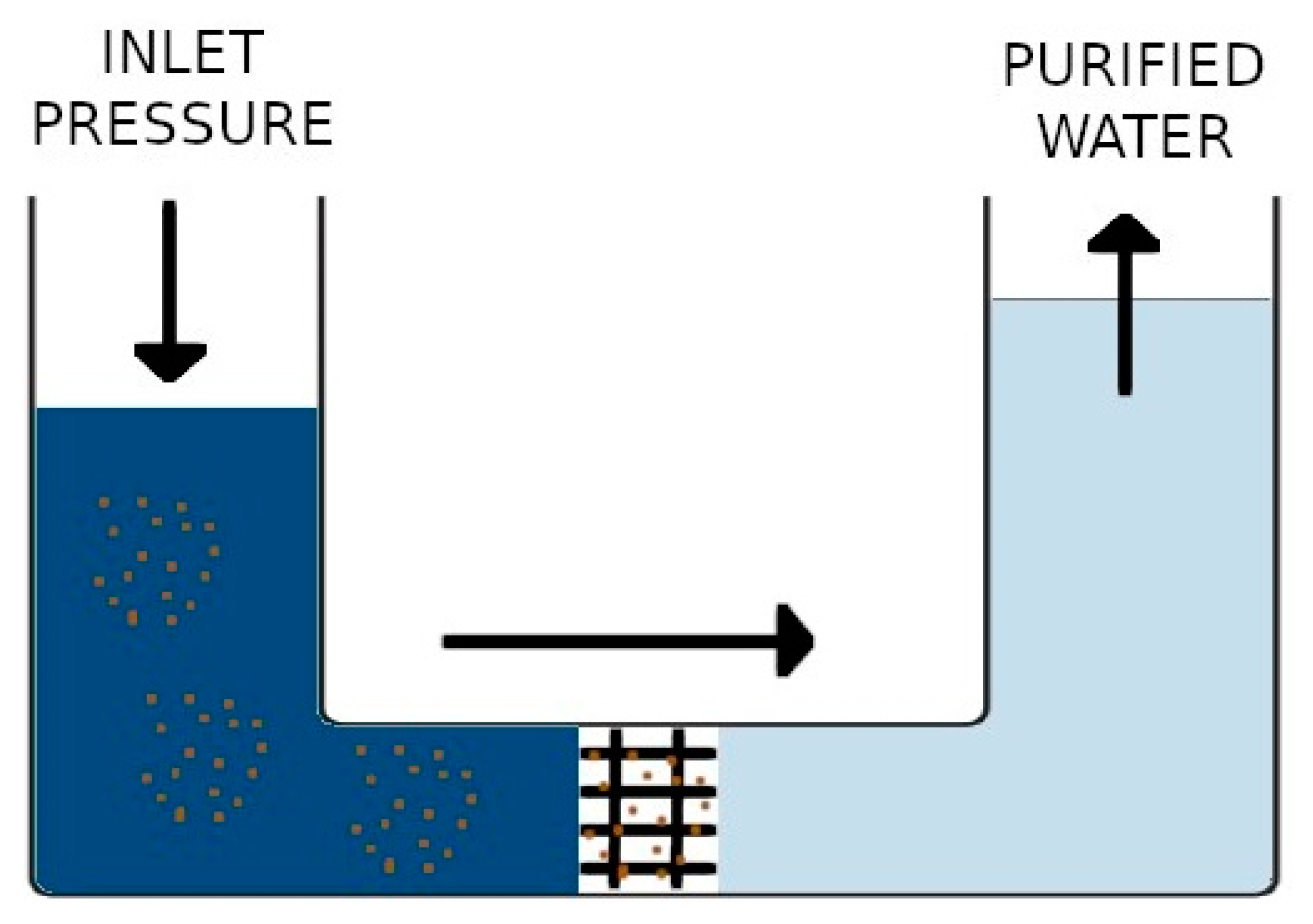
It should be noted that nowadays the implementation of membrane technology at a large scale is a reality at water reclamation and drinking water treatment facilities [3]. Reverse osmosis, which is also known as hyperfiltration, is a process by which solvent molecules are forced from the more concentrated solution into the less concentrated one when a pressure greater than the osmotic pressure is applied. Hence, the reverse osmosis system uses cross-filtration, more commonly called tangential filtration. The greater the concentration, the greater the pressure required. Moreover, the turbulence derived from the induced pressure is strong enough to allow the membrane surface to remain clean. Therefore, another fundamental characteristic of the reverse osmosis process is that it does not alter the characteristics of the product, thus not compromising the subsequent characteristics of the processes that will be implemented in the product. The aim of this process is to obtain a pure solvent by preventing the passage of the solute from one side to the other with a membrane. Figure 1 shows the reverse osmosis process.

The above-described technique not only uses the presence of a physical obstacle to filter the water, but it also uses the membrane to separate the different species based on their different chemical affinities. For instance, in this way only hydrophilic molecules can pass through the membrane.

Reverse osmosis is used in water treatment mainly for two purposes [3]:

• Desalination
• Removal of traces of polluting molecules that could compromise the success of the process and the quality of the process output

For more than a decade now, the reverse osmosis process has been establishing itself as a water desalination process by virtue of its low cost and energy efficiency [4]. Reverse osmosis is also gaining wide acceptance in water desalination plants. In fact, in this field the water purification process allows for the obtaining of drinking water, which is especially useful in geographical areas where drinking water is a scarce resource. Furthermore, as far as energy consumption is concerned, in the last 20 years reverse osmosis ensured an 80% reduction of the energy required for the production of desalinated water compared to other technologies applied for the same purpose [5]. Interesting considerations have been made on the necessity of correct and structured monitoring of the membrane conditions in reverse osmosis processes. The monitoring process is in fact crucial to avoid permanent damage to the membrane itself and to hinder inadequate quality levels and production slowdowns, as previously mentioned [6]. According to the same contribution, it is important to take into consideration the different quality levels of input water at the beginning of a process. However, this procedure makes the monitoring process more complex and delicate. In fact, different characteristics of water entering the system generate different output parameters that must be then contextualized in terms of the time dependence of the parameters. Therefore, according to the characteristics of the input water, the obtained parameters could represent either a healthy or an abnormal state of the machinery. Furthermore, an additional hindering aspect for the analysis is the absence of correct contextualization of the monitored data, which can invalidate the obtained results. For this reason, it is crucial to conduct further research on these types of processes [7].

Many plants use the reverse osmosis process to demineralize water [8]. As previously mentioned, this process is of paramount importance for the quality of the products processed, particularly in pharmaceutical contexts, such as the one under analysis. Consequently, it is crucial to ensure process continuity and a rapid resolution of maintenance problems. Taking into account the level of automation of these systems, reverse osmosis plants can be exposed to faults in several process components that can consequently affect plant operation [9]. The existing literature indicates that the most significant costs in many industrial plants are the maintenance, operating, and energy costs [10]. For this reason, the interest in reverse osmosis has become more and more important since reverse osmosis can guarantee relatively low operating and maintenance costs [11]. As previously mentioned, the reverse osmosis process has a crucial role in pharmaceutical processes, and it is therefore a critical aspect that should be carefully managed in pharmaceutical manufacturing, especially when considering semisolid and liquid products [12]. The issue of maintenance of this installation category is therefore an important and highly debated matter for which several approaches have been suggested over the years [13,14,15]. Nevertheless, the existing literature on the subject of reverse osmosis process monitoring is limited. Recently, a new approach was proposed for fault detection based on a structural analysis approach for an industrial seawater reverse osmosis plant [16]. Another approach proposed hybrid minimal structurally overdetermined sets for hybrid systems formulated as a binary integer linear programming optimization problem [17]. Furthermore, the analysis of the most similar approaches to the one proposed in this paper revealed that the unfold principal component analysis (UPCA) and principal component analysis (PCA) [13,14] were applied for monitoring reverse osmosis processes. However, in this case the application of these two techniques was not considered appropriate since PCA does not allow for the management of process nonlinearities and UPCA is more suitable for batch production, which is absent in the process under analysis. The review of the existing literature on the subject indicates that the reverse osmosis process is nonlinear, as it is described as a set of differential equations [9,18]. This point is particularly interesting because the literature highlights the need to investigate contexts that are increasingly realistic and complex and less ideal and simple, with an eye to data-driven approaches and to the management of data deficiency or incompleteness [19]. This particular feature of the reverse osmosis process motivated the application of a well-known technique in the scenario of fault identification, i.e., the kernel principal component analysis (KPCA). Unlike PCA, KPCA does not neglect the nonlinearities that can be detected in the behavior of the process under examination [20]. In fact, it is interesting to note that the KPCA technique allows for the extraction of nonlinear information from data [21]. As far as the chemical processes are concerned, PCA reveals difficulties in fault detection since it is based on the assumption of linearity of data [22]. However, an interesting limitation that can be found in KPCA is that of data uncertainty management due to, for example, sensor problems or data noise [21]. Besides, KPCA is still critical of incipient failures, i.e., those with small fluctuations and very slow changes [23]. By analyzing the literature on the subject, it is possible to observe that the KPCA has often been modified or used in combination with other techniques to monitor industrial systems, such as Kullback Leibler divergence [23], or more recently combined with deep learning algorithms for degradation assessment and subsequent prognostication of rolling bearings [24]. Moreover, KPCA has been very successfully used both in the field of fault detection and diagnosis for rotating machines given their intrinsic nonlinearity of the process [24]. In fact, KPCA has been applied not only in the field of fault identification but also in the field of fault diagnosis [25]. Furthermore, the application of the KPCA technique does not necessarily require a defined priori of the number of components to be extracted [26]. Moreover, due to its ability to use different kernels, this analysis technique can handle a wide range of nonlinearities [26]. For this reason, KPCA is considered highly user-friendly and appealing in the context of process monitoring.

Taking into consideration the nature and behavior of the process, it is possible to observe a clear temporal correlation of the process variables—typical of chemical process—which should be somehow taken into account as presented, for example, in other contributions and with other techniques, e.g., canonical variate analysis [27], long short-term memory [28], recurrent neural networks [29], or canonical variate dissimilarity analysis [30]. Future research developments in this regard are discussed in the conclusion section.

Finally, another feature that makes this process complex to monitor is the way of recording data. In fact, the monitoring of the examined process is not continuous in time nor at regular time intervals. The available data have been obtained with a sample monitoring of the parameters without the regularity of time intervals for this sampling.

Based on the above-mentioned process characteristics, the paper proposes a KPCA-based reverse osmosis process monitoring approach. However, in order to consider the temporal correlation in the dataset, the entire dataset will not be given as input to the KPCA, neither in training nor in the testing phase. Instead, the past and future correlation matrices of the dataset were calculated and used as input for the application of the KPCA. The advantage of using KPCA in synergy with temporal matrices lies in the fact that KPCA is an established monitoring technique whose results in monitoring dynamic processes have been proven. Moreover, the temporal matrices allow its application to be extended by including information on the time evolution of the analyzed process. Considering the existing literature on the subject, the time dependency in this type of process, which also supports a technique for handling nonlinearities in the process, presents a novel approach that has yet to be investigated. In detail, the approach will be based on two steps:

• Study of the temporal correlation of the process with itself to determine the time intervals to consider for the construction of the past and future matrices
• Application of the KPCA for fault detection using as an input only the past and future matrices constructed in the previous point, not the entire dataset

2. Materials and Methods

2.1. Case Study

As previously stated, the case study analyzed in this paper focuses on the analysis of a water treatment plant that processes the water that is fed into a pharmaceutical production process. The failure management of this system is crucial, since an incorrect operation would imply an injection of contaminated water into the production line. Therefore, the purifying process is of paramount importance, as it prevents contaminated water from being introduced into the production system of a pharmaceutical establishment. It is possible to note that the damage lies both in quality and in the effective possibility of producing a compliant product with considerable economic and production losses due to the discarding of compromised production batches. The considered input parameters in this study are:

• ${\mathrm{x}}_1$ = inlet pressure
• ${\mathrm{x}}_2$ = filtered water pressure
• ${\mathrm{x}}_3$ = filtered elements pressure
• ${\mathrm{x}}_4$ = exhaust flow rate of the filtered elements
• ${\mathrm{x}}_5$ = filtered water flow rate
• ${\mathrm{x}}_6$ = total flow rate
• ${\mathrm{x}}_7$ = temperature

The dataset analyzed was composed of 687 measurements. Of these measurements, 576 were recorded with the machine in normal operating condition and 111 with the machine operating under a failed condition. The failed condition monitored was due to clogging of the filters at the plant inlet. This fault was not induced in the system but occurred naturally during the production process.

2.2. Methodology

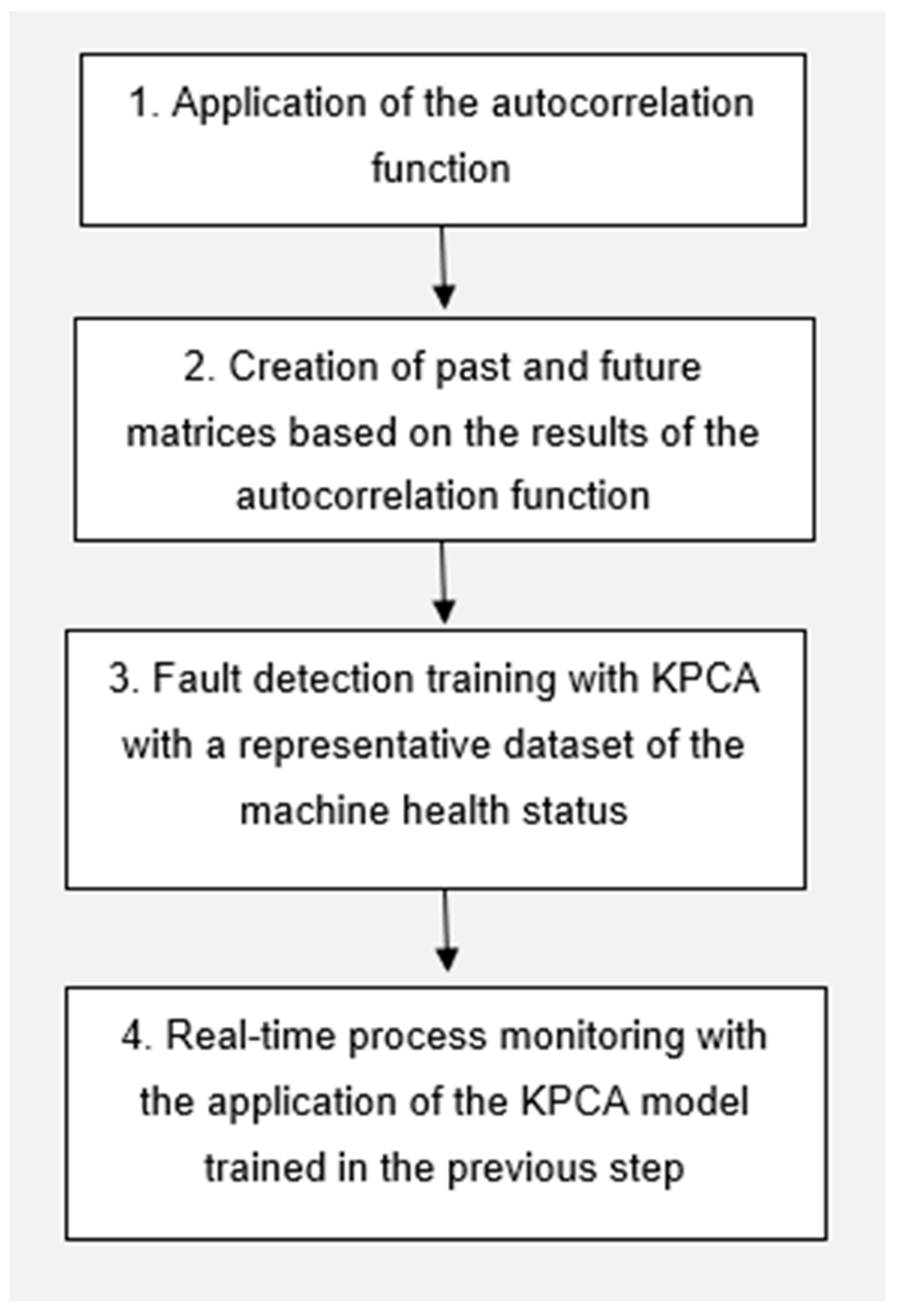
By analyzing the volume of contributions concerning the KPCA, it was considered appropriate to present the steps undertaken to structure the methodology rather than a detailed explanation of how the KPCA works, which can be found in other contributions [26,31]. Figure 2 illustrates the steps followed in the approach presented in this paper.

A fundamental step for the application of the KPCA is the choice of the kernel. Based on the literature review, several approaches can be implemented for this purpose. In the presented paper, the iterative approach was applied since it allows a prompt comparison of the obtained results and it ensures an easily applicable and replicable process of data analysis. The iterative approach is a process of continuous improvement of the model. This means that, in a cyclical process, some steps are carried out more than once with the aim to improve the outcome at each completion. Therefore, by observing the improvements or decline of the results achieved with the model, it is possible to identify the positive or negative changes in the applied kernel. As a result, different kernels were tested for each of the proposed approaches. Moreover, for each approach a parameter optimization process was applied in order to find the kernel and the related parameters that guarantee the best performance.

The different approaches tested refers to the various combinations of past and future matrices that will be subsequently presented.

Specifically, the most popular kernels in the existing literature have been chosen and tested, namely:

• Linear kernel
• Gaussian RBF kernel
• Polynomial kernel
• Exponential kernel
• Sigmoid kernel
• Laplacian kernel

However, considering the peculiarities of each process, digressions on the different outputs obtained with the different combinations of kernels are not discussed in the present paper. In fact, each monitored process is characterized by specific features, and this means that each process responds differently to different kernels applied. In line with this consideration, and according to the applicative nature of the proposed paper, it was not considered appropriate to deepen the theme of the application and the consequent performance obtained with different kernels.

The results presented below refer to the best combination, identified through the performed analysis, i.e., the combination that guaranteed the achievement of the best values for the performance evaluation indices taken into consideration. In this case, the best configuration was the polynomial kernel configuration.

The procedures presented hereafter were performed to confirm the need to apply the above-mentioned methodology. Firstly, an optimization of the application of fault detection with KPCA to the same dataset was performed without using the past and future matrices but using the original dataset with pure monitoring data. The indices used for monitoring were $T^2$ and Q, as presented in [26]. These indices account for two different aspects of the performance of the structured model. $T^2$ represents the variation within the model. It is, in a word, the sum of the normalized squared errors. Referring to what is proposed in [26], $T^2$ is defined as follows (1):

$$T^2=\left[t_1, \dots , t_p\right]{\Lambda }^{-1} {\left[t_1, \dots , t_p\right]}^T$$

(1)

In (1) the principal components t are obtained by projecting ϕ(x) onto the eigenvectors $v_k$ in the feature space, where ϕ(x) is a nonlinear mapping function used to project the input vector to the feature space.

Q, on the other hand, provides another insight into model performance, as it represents how well a new sample fits the constructed model as the squared prediction error.

For an in-depth detail of the calculation of both indicators please refer to [26]. Both indices were assessed with the same metrics, i.e., false alarm rate and the missed detection rate, defined as follows:

• FAR = FALSE ALLARM RATE

  $$\mathrm{FAR}=\frac{n of wrongly identified samples as faults}{total number of fault free samples}$$
• MDR = MISSED DETECTION RATE

  $$\mathrm{FAR}=\frac{n of wrongly identified samples as faults}{total number of fault free samples}$$

The choice of these performance evaluation metrics is clearly defined according to the objectives of the paper. Some of the most commonly used metrics to describe the performance of fault detection analyses are accuracy, precision, sensitivity, specificity, and F1 score [32]. These types of metrics are based on the evaluation of various ratios between the number of true and false positives and true and false negatives. For the case study considered in the paper, the false positives were the data mislabeled as faulty, the false negatives were the data mislabeled as healthy, the true negatives were the data correctly labeled as healthy, and true positives were those correctly labeled as faulty. However, considering the applicative nature of the paper and the fact that it is well embedded in a real industrial context, it would be interesting to apply metrics that would ensure a quicker and easier way to contextualize interpretation of the results. For this reason, in the case study under consideration false alarms and unidentified faults were considered as evaluation metrics, as also proposed in other contributions, such as [33]. For the sake of clarity, however, and to facilitate the reader’s understanding, the results will also be presented in the form of confusion matrices with subsequent evaluation of accuracy, precision, and sensitivity. Following the optimization process, both indices presented the results, which are summarized in

Table 1. KPCA results without the proposed methodology.

	FAR	MDR
$T^2$	16.5%	80%
Q	4.5%	3%

and

Table 2. Results analysis without the proposed methodology.

	TP	TN	FP	FN
$T^2$	23	481	95	88
Q	108	550	26	3

.

Analyzing the results presented, the accuracy, precision, and sensitivity of this first test are reported below (

Table 3. Accuracy, precision, and sensitivity without the proposed methodology.

	Accuracy	Precision	Sensitivity
$T^2$	73.3%	19.49%	20.7%
Q	95.77%	80.59%	97.29%

).

Before proceeding to the description of the methodology presented and to the connected results, the results shown in Table 1 should be briefly discussed. Firstly, by observing the $T^2$ results, it is possible to note that they are absolutely not acceptable, especially due to the lack of identification of data representative of a failure. Secondly, the results achievable with Q are not inadequate, but they could be improved with the application of the proposed methodology. The suggested improvement will be presented in the subsequent sections.

2.2.1. Application of the Autocorrelation Function

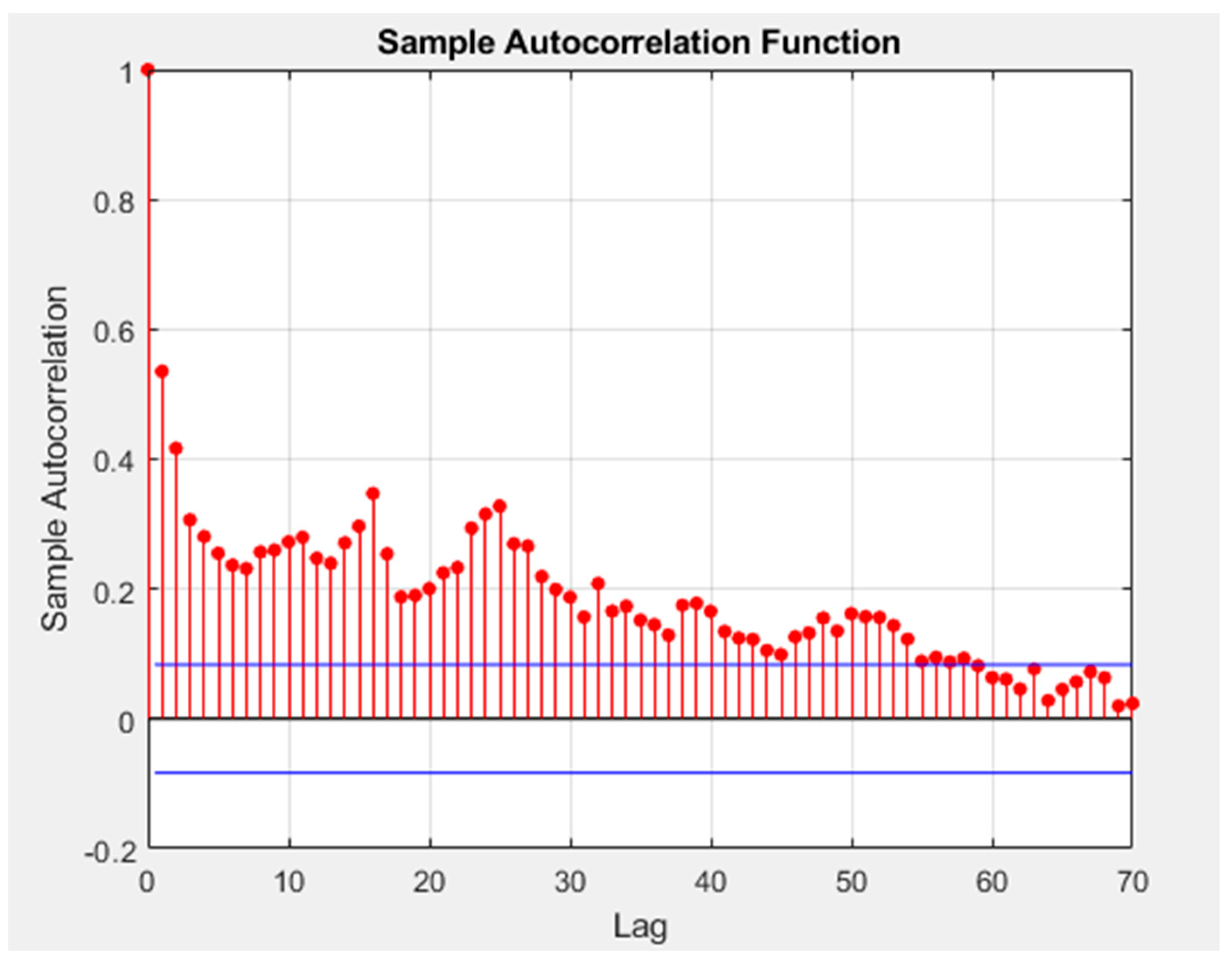
First of all, according to the results presented in Figure 2, the autocorrelation function should be applied. In fact, the number of periods of interest for the construction of the past and future matrices was defined by using the autocorrelation function of the root summed squares of all variables in the training dataset in a confidence bound of ±5% [34]. The purpose of the application of the autocorrelation function was to identify significant time intervals. In fact, the autocorrelation function detects the duration of the period during which a signal is self-correlated. The results of the application of the autocorrelation function are shown in Figure 3.

By examining Figure 3 and the results obtained from the application of the autocorrelation function, it was possible to observe that the time intervals of interest considered 59 periods. This is the value of p and f that was considered in all the implemented tests, starting from the one presented in Table 1.

2.2.2. Creation of Past and Future Matrices Based on the Results of the Autocorrelation Function

The calculation of the past and future matrices is used as input for the training phase of the KPCA and then as input for the actual testing and monitoring phase. In this phase, the authors computed both past and future matrices since various tests were subsequently implemented. The tests were necessary to determine whether it was appropriate to only use the past matrices of the datasets for the application of the KPCA or a combination of past and future matrices. The past and future matrices were calculated as presented in the next section of this paper.

Firstly, two data matrices were generated starting from the measured data $y_t$∈$R^n$, with n representing the process variables and t representing the sampling time. This is possible by expanding each sampling, including p past samples and f future samples. After the definition of these two parameters, which should have the same value, the future and the past sample vectors $y_{f,t}$ ∈ $R^{fn}$ (2) and $y_{p,t}$ ∈ $R^{pn}$ (3) were constructed.

$$y_{f,t}={\left[y_{ t+1, } y_{t+2, }\dots , y_{t+f-1 }\right]}^{\mathrm{T}}$$

(2)

$$y_{p,t}={\left[y_{t-1, } y_{t-2, }\dots , y_{t-p }\right]}^{\mathrm{T}}$$

(3)

To avoid the influence of variables with bigger absolute values on fault detection, $y_{f,t}$ and $y_{p,t}$ were normalized to mean zero vectors ${\widehat{y}}_{f,t}$ and ${\widehat{y}}_{p,t}$. The latter at different sampling times were then rearranged to create the future observations matrix ${\widehat{Y}}_f$∈ $R^{fnXN}$ (4) and the past observations matrix ${\widehat{Y}}_p$ ∈ $R^{pnXN}$ (5).

$${\widehat{Y}}_f=[{\widehat{Y}}_{f,t+1},{\widehat{Y}}_{f,t+2},\dots ,{\widehat{Y}}_{f,t+N}]$$

(4)

$${\widehat{Y}}_p=[{\widehat{Y}}_{p,t+1},{\widehat{Y}}_{p,t+2},\dots ,{\widehat{Y}}_{p,t+N}]$$

(5)

In (4) and (5) N = m − p − f + 1, with m representing the number of total samples in $y_t$.

2.2.3. Training and Test of the KPCA Monitoring Model

The two final steps of the methodology, i.e., the training and the test of the KPCA monitoring model, tend to be similar and it is therefore useful to comment on them together. The expression “training” refers to the part in which the model is trained using data extrapolated from the operating machinery under normal conditions, aimed at defining the control thresholds of the process. Consequently, as shown in Figure 2, it should be pointed out that the training part of the model was performed in each of the tested combinations using only data representative of a healthy state of the machine in order to correctly calculate the thresholds of $T^2$ and Q [26]. On the other hand, the expression “test” describes the actual process monitoring, i.e., the analysis of process data based on the thresholds previously defined, when it is still not known whether the data fed into the model are healthy or faulty.

Throughout this step, the most suitable kernel for the monitored process is defined. In general, it is crucial to obtain the following information to implement the training and testing phases:

• p and f value, based on the autocorrelation function results
• Matrices of past and future measurements, calculated from the values identified for p and f, for both the training and test datasets
• Kernels identified as possibly suitable for the process to be monitored

The third point is the most demanding. In fact, while the first two points are a simple application of algorithms with an output that is easy to interpret and ready to use, the third point requires a different approach to define the most suitable kernel for the monitored process, as well as the parameters to be set in the kernel. For the definition of the most suitable kernel, the following approach was adopted: after the definition of p and f, with the consequent calculation of the matrices of past and future measurements, these two steps of the methodology were considered defined and immutable. Moving on to the choice of the kernel, several kernels were selected based on the literature review, as indicated in Section 2.2. Subsequently, all the selected kernels were applied, both in the training and testing phases, with different settings to identify the most suitable kernel and, consequently, the best setting to monitor the analyzed reverse osmosis process.

After identifying the kernel to be applied, the different combinations of past and future matrices for both the training and test phases were tested. For the sake of completeness, the logical path that led to the definition of the combinations tested will be explained in the following section of this contribution. Furthermore, five tests were performed with five different combinations of past and future measurement matrices for the training part and the testing part, i.e., for the real monitoring part of the process. First of all, it was ascertained that within the representative data of a state of health it was possible to identify a trend of degradation, traceable in the same way in the actual monitoring data of the process. This led to the development of the first test, in which the search for this trend of degradation of the machinery resulted in the sole use of the matrices of past measurements both to train the model and subsequently to monitor the process concretely. The two additional implemented tests, for which further and more detailed explanations will be given in the next section, were based on the idea that it is possible to identify unexpected oscillations that allow for the identification of the onset of a fault by jointly analyzing the matrix of past and future measurements. This hypothesis led to an analysis whether or not the difference between the matrix in future and past measurements could be a good input for monitoring with the KPCA. In this regard, two tests were implemented: one in which this input was used in both the training and testing phases, and the other in which only the matrix of past measurements was used in the testing phase. The rationale behind this choice lies in the fact that it was considered important to verify the response in the testing phase both using and not using this difference. When considering only the data measured in conditions of normal operation of the machine, the training phase presented a greater regularity than the testing phase, which instead presented the onset of the fault. The objective of this differentiation was therefore to verify whether the difference between the matrix of future and past measurements could be only a good input for the calculation of the control thresholds or whether it could also play an active role in the real process monitoring phase. The final test group followed the same logic that was applied to the groups where the difference between future and past matrix measurements was used. This time, however, the analysis aimed at defining whether the relationships between future and past measurements could be made explicit by summing the two matrices rather than by subtracting them. In light of this, it is possible to state that the applied logic and reasoning are essentially the same, but with different means of information conveyance.

3. Results

In the first test performed, only the past matrix of the dataset was considered both for the training phase and for the testing phase. However, this option proved disadvantageous in terms of results, which are summarized in

Table 4. KPCA only with past matrix.

	FAR	MDR
$T^2$	100%	0%
Q	100%	0%

,

Table 5. Results analysis only with past matrix.

	TP	TN	FP	FN
$T^2$	111	0	576	0
Q	111	0	576	0

and

Table 6. Accuracy, precision, and sensitivity only with past matrix.

	Accuracy	Precision	Sensitivity
$T^2$	16.15%	16.15%	100%
Q	16.15%	16.15%	100%

. In fact, with this approach KPCA was completely unable to distinguish between the state of health and the state of failure of the machinery, ending up labeling everything as a state of failure. As a consequence, a 0% rate of faults and a 100% rate of false alarms were identified. In conclusion, it is possible to state that this approach was completely unenforceable. In this case, the response of the two indices was the same, in contrast to the results obtained from the previous analysis (Table 1).

The results obtained from this analysis cannot be considered acceptable, even considering the benchmark situation, i.e., the situation in which the entire dataset without any manipulation is used as an input for the KPCA. This particular benchmark situation was chosen since it represented the outcome that needed to be overcome. Therefore, it was considered appropriate to implement new tests. In this case, due to the need to combine the information in the matrix of past measurements and of future measurements, it was considered appropriate to examine some arguments regarding the canonical variate dissimilarity analysis (CVDA), which can be defined as an of evolution of the CVA. The main difference between CVA and CVDA lies in the fact that the latter extends CVA with a new index—which in this paper will be referred to as D—based on the difference between the past-projected and future-projected canonical variables [30]. The idea behind this technique is based on CVA’s ability to find correlations between past and future datasets in light of the possibility to identify small deviations from the correct trend of the parameters considering how well one parameter can predict future canonical variables based on the previous ones [30]. In this technique, the difference between the matrix of past measurements and that of future measurements is taken into account in order to calculate the health indices during the process monitoring phase. Obviously, in CVDA a simple difference between the two matrices is not applied. However, considering the purpose of the paper, the fault detection model was trained by giving it as input only the difference between the matrix of future measurements and that of past measurements. In the first case, only the matrix of past measurements will be given for testing and therefore for actual monitoring. In the second case, what is proposed for the training will also be reproduced for testing, thus computing the difference between the matrix of future measurements and that of past measurements.

For the sake of clarity, the difference between the matrix of future measurements and the matrix of past measurements is defined by the following procedure.

Firstly, the difference between the matrix of past measurements is represented by ${\widehat{Y}}_p$, while the matrix of future measurements is represented by ${\widehat{Y}}_f$. Subsequently, considering, for example, a matrix ${\widehat{Y}}_p$ of size 2 × 2 (6) and a matrix ${\widehat{Y}}_f$ of size 2 × 2 (7) asfollows:

$${\widehat{Y}}_p=\left(\begin{array}{cc}{a}_{11}& a_{12}\\ a_{21}& a_{22}\end{array}\right)$$

(6)

$${\widehat{Y}}_f=\left(\begin{array}{cc}{b}_{11}& b_{12}\\ b_{21}& b_{22}\end{array}\right)$$

(7)

It is possible to define the matrix C, obtained by subtracting the matrices ${\widehat{Y}}_f$ and ${\widehat{Y}}_p$, as (8):

$$C=\left(\begin{array}{cc}{b}_{11}-a_{11}& b_{12}-a_{12}\\ b_{21}-a_{21}& b_{22}-a_{22}\end{array}\right)$$

(8)

Moving on to the analysis of the obtained results, the second investigated approach analyzed the difference between future and past matrices in both training and test datasets. The achieved results are presented in

Table 7. KPCA with the difference between the past and future matrix for both training and test.

	FAR	MDR
$T^2$	17.8%	59.6%
Q	4.8%	7.6%

,

Table 8. Results analysis with the difference between the past and future matrix for both training and test.

	TP	TN	FP	FN
$T^2$	45	473	103	66
Q	103	548	28	8

and

Table 9. Accuracy, precision, and sensitivity with the difference between the past and future matrix for both training and test.

	Accuracy	Precision	Sensitivity
$T^2$	75.4%	30.4%	40.5%
Q	94.7%	78.6%	92.8%

.

It is possible to note that the results obtained from this analysis are better that those presented in Table 4. Consequently, this improvement indicates that considering both the matrix of past and future events increases the information available, and it also increases the readiness of the model. However, the results are still worse than the ones presented in Table 1, and it is therefore necessary to investigate other solutions. In this regard, two considerations should be made. The first one concerns the overall error rate of this model, which is still unacceptable and requires further investigation about the achievable results. The second one concerns the sensitivity analysis of the two indices. In fact, $T^2$ usually provides significantly better results than Q, while in the presented case the results are inverted.

In the third approach analyzed, the input of the training phase was the difference between the matrix of future measurements and that of past measurements, while for the test phase only the matrix of past measurements was given as the input to the model. The obtained results are presented in

Table 10. KPCA with the difference between the past and future matrix for training and only past matrix for test.

	FAR	MDR
$T^2$	0%	27%
Q	0%	4.5%

,

Table 11. Results analysis with the difference between the past and future matrix for training and only past matrix for test.

	TP	TN	FP	FN
$T^2$	81	576	0	30
Q	106	576	0	5

and

Table 12. Accuracy, precision, and sensitivity with the difference between the past and future matrix for training and only past matrix for test.

	Accuracy	Precision	Sensitivity
$T^2$	95.6%	100%	72.97%
Q	99.27%	100%	95.49%

.

It is interesting to note that this combination of past and future matrices has significantly increased the achievable results, making them highly performant. Moreover, this is the first combination of matrices that gives better result than those presented in Table 1. However, even in this case Q performed better than $T^2$, which is unusual.

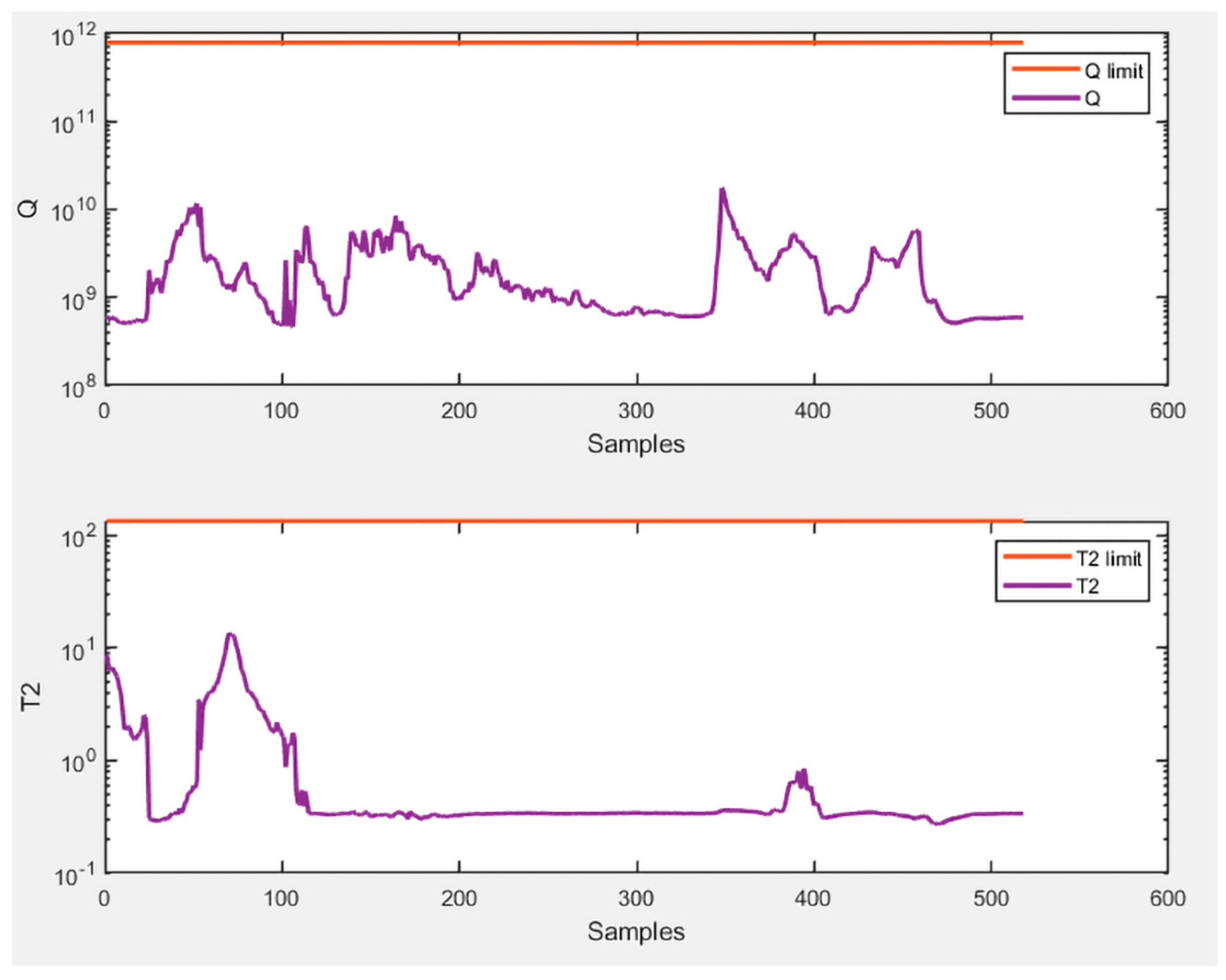
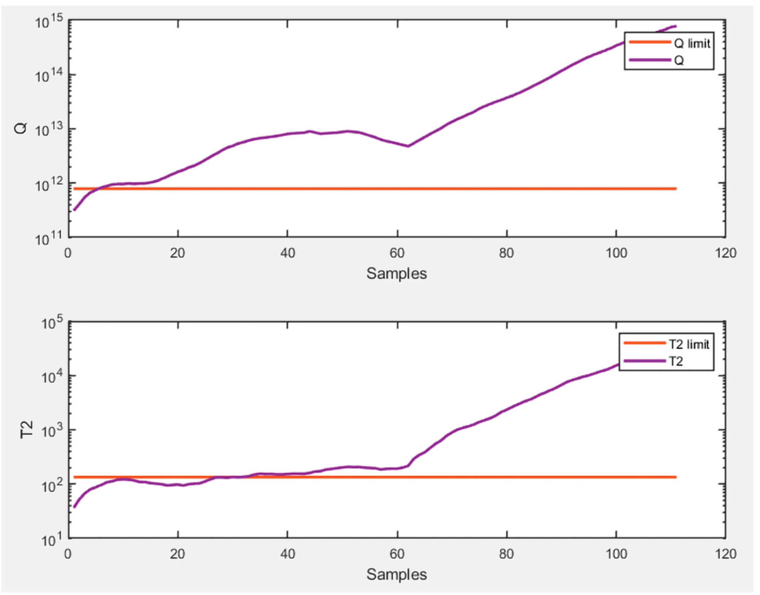
Despite that, the results obtained from this approach are excellent, and the graphs of $T^2$ and Q are therefore presented below to provide a visual oversight of the success of monitoring with this technique. Specifically, Figure 4 shows the monitoring of healthy data and Figure 5 shows the monitoring of faulty data.

The good results obtained with the combination of the past and future matrices, specifically their difference, allow us to make some interesting considerations. For instance, it would be interesting to see the results of the analysis by calculating the sum and not the subtraction of the matrix of past measurements and that of future measurements.

The tests presented hereafter provide an answer to this question, thus finally leading to the definition of the best model. However, it was already stated that both approaches tested with the sum of the matrix of past and future measurements guaranteed better results than the benchmark situation (Table 1).

Based on these considerations, in the fourth test performed for both the training and test input, the sum of the past and future matrices was used. The results are shown in

Table 13. KPCA with the sum of the past and future matrix both for training and test.

	FAR	MDR
$T^2$	20%	0%
Q	6.1%	0%

,

Table 14. Results analysis with the sum of the past and future matrix both for training and test.

	TP	TN	FP	FN
$T^2$	111	461	115	0
Q	111	541	35	0

and

Table 15. Accuracy, precision, and sensitivity with the sum of the past and future matrix both for training and test.

	Accuracy	Precision	Sensitivity
$T^2$	83.3%	49.1%	100%
Q	94.9%	76%	100%

.

By observing on the obtained results—presented in Table 13—it is possible to notice that the problem deriving from this approach is represented by the false alarms and not by the failure identification. In the same way, it is interesting to notice that, like for the previous analyses, Q shows globally higher results, while with MDR the two indices had the same results, and with FAR, Q obtained better results. Although the obtained results are good, it is possible to observe a worsening compared to the data presented in Table 10 which are so far the best result, i.e., results where the difference between the matrix of future measurements is used as input for the training and the sole matrix of past measurements is used as input for the test.

Furthermore, similarly to what was previously done for the difference between the time matrices, this paper investigated the way in which the results can change for the sum of the time matrices if the sum of the matrix of past and future measurements is only entered as the input in the training phase, while only considering the matrix of past measurements in the testing phase. Finally, this attempt allowed us to obtain the best results. In fact, the results achieved with this approach were the best results obtained overall and they are summarized in

Table 16. KPCA with the sum of the past and future matrix for training and only past matrix for test.

	FAR	MDR
$T^2$	0%	1%
Q	0%	6%

,

Table 17. Results analysis with the sum of the past and future matrix for training and only past matrix for test.

	TP	TN	FP	FN
$T^2$	110	576	0	1
Q	104	576	0	7

and

Table 18. Accuracy, precision, and sensitivity with the sum of the past and future matrix for training and only past matrix for test.

	Accuracy	Precision	Sensitivity
$T^2$	99.85%	100%	99%
Q	98.98%	100%	93.69%

.

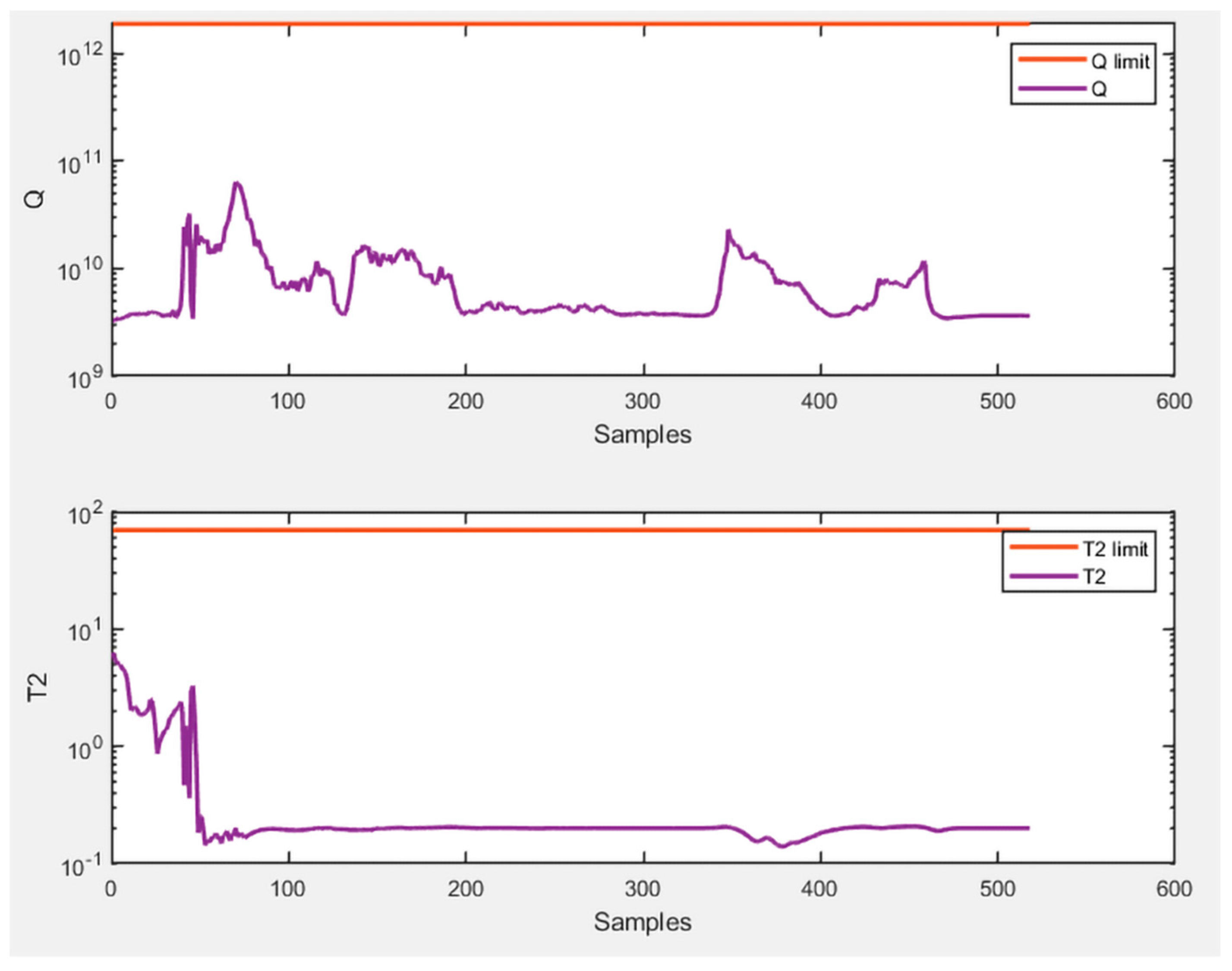
Comparing the results presented in Table 16 with those shown previously, it is possible to observe that the results achieved with this last configuration are clearly better than the previous ones. In fact, $T^2$ had almost perfect results, both in terms of false alarms and unidentified faults. Moreover, Q presented 0% false alarms, but 6% unidentified faults. In this case, $T^2$ presented better results overall, as expected. In light of the achieved results, the graphs of $T^2$ and Q related to this approach are presented to provide a clear representation of the monitoring applied in this technique. 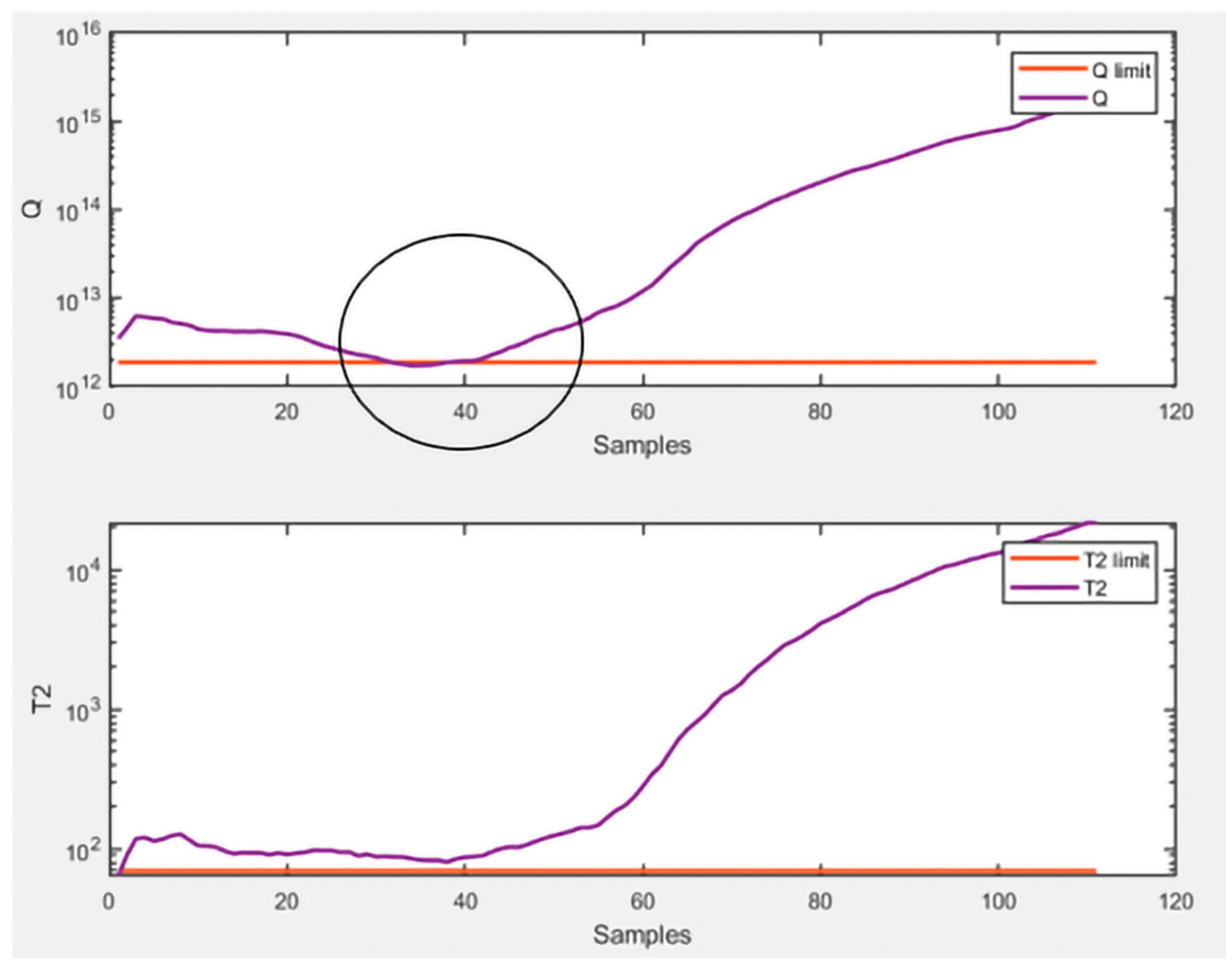Specifically, Figure 6 shows the monitoring of healthy data and Figure 7 shows the monitoring of faulty data.

The circle inserted in Figure 7 represents the section of data representative of a failure state that has been mislabeled as representative of a healthy state by Q.

4. Discussions and Conclusions

This study proposes the application of KPCA to identify faults in a reverse osmosis plant operating in the pharmaceutical industry. Specifically, the purpose of the process is to purify the water before entering it into the processing cycle. The process has many critical issues regarding its monitoring, thus making it complex to perform proper fault detection.

It is interesting to note that the monitoring criticalities come from two different points: some are intrinsic to the process itself; others instead are dependent on the management chosen for the implementation of the monitoring process. In the first case, the process itself operates under conditions that vary over time, since the characteristics of the input water are different and discontinuous over time. This means that different characteristics of the input water have different responses of the monitored parameters. Therefore, an incorrect analysis of these differences can lead to an incorrect analysis of the health state of the machinery. Other critical monitoring issues, on the other hand, are induced externally and do not depend on the process itself. In fact, the monitoring and the consequent recording of the parameters is neither continuous in time nor determined with regularity. The sampling is at irregular and undefined intervals, introducing into the system a discontinuity of data that can hide necessary information for correct data analysis. In conclusion, the process is highly dynamic and time-variant.

Considering the dynamic nature of the process, this paper proposes the application of KPCA for monitoring and fault detection in this process. However, the time-variability makes it necessary to examine other considerations on how manage and consider the variability in the phase of fault detection. This analysis led to the core part of the paper, which suggested different combinations of past measurement matrices and future measurement matrices to be included as input for the subsequent fault detection with KPCA. This solution, which opens several future research scenarios, allowed for inclusion in the KPCA the issue of temporal dependence of the process as well.

Several combinations were tested, specifically:

• Only the past matrix of the dataset both for the training phase and for the testing phase
• The difference between future and past matrices both for training and test
• The difference between the matrix of future measurements and that of past measurements for the training phase, while for the test phase only the matrix of past measurements
• The sum of the past and future matrices both for the training and test
• The sum of the past and future matrices for the training and only the past matrix for the test

For the evaluation of the results with the various approaches tested, the initial situation was considered to be that in which the KPCA was trained with the entire dataset without any form of evaluation of the temporal relationships present in it. This situation, whose results are presented in Table 1, was therefore defined as the benchmark situation, i.e., the situation that needed to be overcome.

Firstly, it is interesting to note that the approach in which the training process was performed only with the matrix of past measurements (Table 4) was the least effective, with completely unacceptable results. Moreover, this approach produced results worse than those presented in the benchmark situation alongside the approach in which both the training dataset and the test dataset were a result of the subtraction between the matrix of future measurements and the matrix of past measurements (Table 7).

It is interesting to note that the results show that the use of the matrix of future measurements is limited to the training phase. In fact, its use in the test phase, i.e., in the real monitoring phase, compromised the achievable results. In general, the joint use of information obtained from past and future measurements increased the predictive power of the model. Moreover, it should be noted that the situation in which the two matrices considered were summed was more predictive than when the difference was considered. This topic should require further investigation. In conclusion, regardless of the best resulting combination, it is possible to state that inserting something that allows taking into account the temporal correlation in the data increases the analysis of fault detection subsequently implemented with the KPCA.

By observing the obtained results, the presented proposal could be suitable for dynamic and time-variant production processes. In fact, considering the noncapillarity of monitoring for the analyzed process, it is possible to state that this characteristic of the process indicates that good results in terms of monitoring accuracy can be obtained in processes with dynamic and variable characteristics over time where monitoring is carried out more frequently and regularly. However, there are some limitations. The first limitation is that the production process is continuous, i.e., there are no production batches and therefore no downtime between batches for operations such as cleaning the machinery and subsequent setup for the start of new production. This characteristic of the process does not allow affirmation, to the present date, of what results and what monitoring accuracy could be obtained in a batch process by applying the proposed monitoring technique. The second limitation concerns the role of the monitored process. As previously described, the reverse osmosis process analyzed in this contribution engages with purifying water entering a pharmaceutical production process. However, due to the characteristics of the process, it is not possible to say with certainty whether the same process that was applied for the purification of wastewater of a pharmaceutical plant could be successfully monitored by applying the same methodology. These two main limitations will surely inspire future research developments.

The obtained results raise interesting considerations, which open scenarios for future research developments. As mentioned in the introduction section, other interesting techniques allow the prevention of the loss of information from a complete temporal contextualization. Therefore, firstly it would be interesting to understand how the results achieved on the relationship of KPCA with the temporality of the process can be exploited to develop methodologies that jointly use KPCA and techniques that have an inherent analysis of temporal correlations in the dataset. A second point that should be analyzed with greater attention in future research developments is the application of the methods proposed in productive contexts that present characteristics of different processes, even if remaining in contexts of time-variant processes. For instance, multiphase processes or processes in which the products processed are not always the same. Finally, it would be interesting to further research the different response of the two indices obtained in the proposed situations, i.e., why, in some cases, Q performed clearly better than $T^2$.