Optimization of 3-DoF Manipulators’ Parasitic Motion with the Instantaneous Restriction Space-Based Analytic Coupling Relation

Featured Application

Velocity-level parasitic motion optimization is performed based on the instantaneous restriction space analysis. The manipulator whose parasitic motion is successfully eliminated from the workspace has tremendous benefit for robotic assistive surgery, precision machining devices, and other applications that are critical for manipulators with parasitic motion.

Abstract

This paper presents a velocity-level approach to optimizing the parasitic motion of 3-degrees of freedom (DoFs) parallel manipulators. To achieve this objective, we first systematically derive an analytical velocity-level parasitic motion equation as a primary step for the optimization. The paper utilizes an analytic structural constraint equation that describes the manipulator’s restriction space to formulate the parasitic motion equation via the task variable coupling relation. Then, the relevant geometric variables are identified from the analytic coupling equation. The Quasi-Newton method is used for the direction-specific minimization, i.e., optimizing either the x-axis or y-axis parasitic motion. The pattern-search algorithm is applied to optimize all parasitic terms from the workspace. The proposed approach equivalently describes the 3-PhRS, 3-PvRS, 3RPS manipulators. Moreover, other manipulators within a similar category can be equivalently expressed by the proposed method. Finally, the paper presents the resulting optimum configurations and numerical simulations to demonstrate the approach.

1. Introduction

In recent years, the deployment of lower DoF mechanisms has grabbed the attention of industries and academia due to its interesting properties such as lower cost, kinematic simplicity, fast dynamic response and higher accuracy. For several applications, such as pointing devices, surgical robots, parallel kinematic machines (PKMs), parallel manipulators (PMs) with less than six DoFs can be preferable [1,2,3,4,5]. Because such tasks can be well performed with manipulators having less than 6-DoFs. For example, surgical devices require 4 DoFs at most including one external yaw motion of the tool [6].

Lower mobility PMs as a pointing device:Replacing conventional antenna and telescope positioning methods with PMs dates back to 1980 when first suggested by Fichter and McDowell and later continued by Jones at the Canterbury University [7]. Pointing devices often operate in a complex environment that could heavily affect their accuracy, such as telescopes on satellite continuously changes its pose in relation to the telescope mounted on the ground. However, these devices require higher accuracy and precision to guarantee strong signals in tracking and communication. To ensure the pointing precision under complex operational environment, engineers employed 6-DoFs PM instead of the conventional mounting methods [8,9,10]. Yu et al. introduced a new 6-PSS (prismatic-spherical-spherical) telescope’s secondary mirror alignment mechanism [8]. Sun et al. proposed another 6-DoFs hybrid manipulator for pointing and positioning purposes in aerospace applications [11]. However, manipulation of the secondary mirror of the telescope requires 3-DoFs at most [12]. The remaining degrees of freedom of the manipulator are to avoid singularities. But singularity can be handled by PMs with less than 6-DoFs [12,13]. To avoid the use of such complicated manipulators for lower DoFs tasks, researchers shifted their attention to fewer DoFs mechanisms. Carretero et al. designed a 3-PRS (prismatic-revolute-spherical) manipulator to perform tip/tilt pointing (2 rotational freedoms) and focusing (1 translational freedom) for the secondary mirrors of a Cassegrain telescope [12]. In 2008, a 3-PRS PM was proposed for orienting television satellite antenna [14]. Likewise, the high-performance antenna pointing device (3POD) in a micro-gravity environment was proposed by CENS [13].

Lower mobility PMs as high precision PKMs: PKMs use their actuators working side-by-side to enhance rigidity, fast dynamic response, and accuracy. Due to these advantages, the interest has increased both in academia and industry to use lower mobility PMs as a machining device. The first PKM was introduced at the international machine tool show (IMTS) in 1994. Along that track, there have been intensive research and innovations to meet the conceptual potentials of PKMs [15,16,17,18]. In 2016, the most successful sprint Z3 [19] of the Ecospeed series from Starrag Group had received significant orders in the double-digit million from customers. This success indicates the Ecospeed series with sprint Z3-head has become a choice to achieve 5-axis precision machining in spacecraft and automobile industries. Inspired by Z3-head, Tianjin university developed a PKM with identical motion but with RPS(Revolute-Prismatic-Spherical) joint arrangements in a limb [18]. Both manipulators are extensively studied and are the most used examples to demonstrate different theoretical and experimental approaches.

Lower mobility PMs as surgical devices: One of the medical industry’s growing trends is to use robotic-assisted surgery to take advantage of parallel manipulators’ high accuracy and accessibility. Robots in the medical sector can help surgeons handle routine tasks, complement their skills with manipulators’ accuracy and repeatability, and several researchers focused on exploring PMs’ capabilities in medical applications. Guaranteeing manipulators’ successful usage in the medical field requires few critical requirements to be fulfilled, such as simple operation, efficient control, limited workspace, safe behaving near the singular configurations, etc. Considering the PMs promising features to achieve the medical sector’s requirements, several researchers are developing surgical lower-mobility PMs [20,21].

1.1. The Effect of Parasitic Motion on the Application of Lower Mobility Parallel Manipulators

The applications of robotic manipulators described above require lower DoFs with higher accuracy. Thus, researchers showed keen interest in the use of PMs with lower DoFs instead of the serial ones. Even though parallel manipulators are comparatively accurate enough, a hidden property of lower mobility PMs named parasitic motion can considerably affect accuracy [12]. Parasitic motion is a small dependent movement that occur in the restricted DoFs due to the nature of constraint [12]. For the applications that require higher precision, such as machining, pointing devices, and robotic surgery, parasitic motion causes accuracy problems and control complexity [22]. Because parasitic motion is an unwanted auto-generated movement only to satisfy the structural constraint, and the internal controller cannot correct it.

Therefore, researchers aim to describe parasitic motion, introduce methods to remove the parasitic terms, and invent manipulators without parasitic movement considering various applications sensitive to this natural behavior [12,21,22]. Through the extensive research carried out to define and analyze parasitic motion, Carretero et al. were the first to address it appropriately at the position-level [12]. Their study has also introduced the optimal configuration of a 3-PRS manipulator that minimizes this undesired motion. Later in 2011, Li. et al. [22] also investigated 3-PRS manipulator without and with small amplitude parasitic motion using different limb arrangements. In 2010, Li and Hervé synthesized 1T2R manipulators without parasitic motion [18]. Qu et al. also introduced a method to remove the parasitic motion of 3-UPU by adding a redundant active leg [23]. A simplified method to describe the rotational parasitic motion was introduced by Liu et al. in 2008 [24]. However, the proposed approach is also at the position-level.

In this study, the optimum geometric parameters are obtained purely at the velocity level. Deriving the parasitic motion equation at the velocity level avoids unnecessary explicit position relation coverage. It also suits the commonly used velocity-level control scheme. Previously, the procedure had to start from the position-level relations. However, that is ineffective for someone who does not necessarily need the position information. Note that the parallel manipulator’s control scheme is commonly based on the velocity information since the theory for the velocity analysis is well-established for such mechanisms. Also, embedding the constraint information in the position equation is not uniformly applicable for all manipulators since it is obtained differently for each mechanism. The analytic constraint equation used to formulate parasitic velocity is obtained via screw theory using instantaneous restriction and motion spaces [25,26]. Consequently, the manipulators that optimize the parasitic velocities are obtained.

Moreover, the paper introduces an enhanced performance manipulator without parasitic motion after the performance evaluation of optimized manipulators.

1.2. Description of Example Manipulators

For the example manipulators used in this paper (Figure 1, Figure 2 and Figure 3), the fixed and moving platforms are described by the frames $\left\{O\right\}$ and $\left\{O^{\prime }\right\}$, respectively. The orientation of the moving plate with respect to the base plate is represented by:

$$\mathit{R}={\mathit{R}}_y\left(\theta \right){\mathit{R}}_x\left(\psi \right){\mathit{R}}_z\left(\varphi \right),$$

(1)

whereas the position of the moving plate with respect to the base is described by a vector $\mathit{p}$. Considering the moving plates as a rigid plane, the position of spherical joints is described by the vector ${\mathit{a}}_i$, which is directed from $O^{\prime }$ to $A_i$ and written as follows:

$${\mathit{a}}_i^{\prime }={\mathit{R}}_z\left({\alpha }_i\right){\mathit{T}}_x\left(r_p\right).$$

(2)

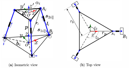
Figure 1. Kinematic architecture of the 3-RPS manipulator.

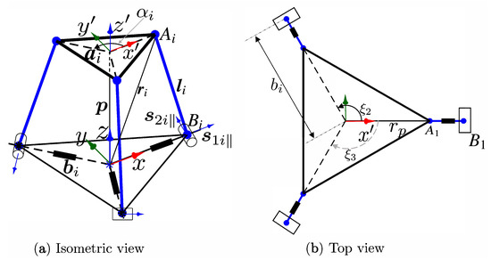
Figure 2. Kinematic architecture of the 3-PhRS manipulator.

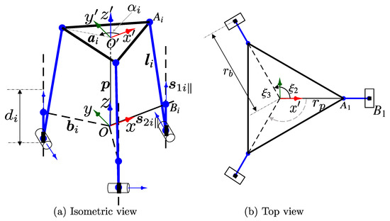
Figure 3. Kinematic architecture of the 3-PvRS manipulator.

Variable $r_p$ in Equation (2) implies the radius of the moving platform’s circumscribed circle and ${\mathit{T}}_x(·)$ represents a translation vector in the x- direction by the specified magnitude, in this case $r_p$. The angle ${\alpha }_i$ defines the location of three spherical joints measured from the positive x-axis parallel to the moving platform and is given as:

$${\alpha }_i=(i-1)\frac{2\pi }{3},\mathrm{for}i=1,2,3.$$

(3)

whereas the revolute joints located on the fixed platform can be measured by the angle ${\xi }_i$ from the positive x-axis and parallel to the fixed platform as in Equation (4).

$${\xi }_i=(i-1)\frac{2\pi }{3},\mathrm{for}i=1,2,3.$$

(4)

The vector from $\left\{O\right\}$ to $\left\{B_i\right\}$ can be denoted by ${\mathit{b}}_i$. So, it can be described by the following relation:

$${\mathit{b}}_i={\mathit{R}}_z\left({\xi }_i\right){\mathit{T}}_x\left(b_i\right).$$

(5)

Note that $r_p$ and $b_i$ of Figure 1 and Figure 2 are initially the same and can be equally represented in Equation (5). In solving the inverse kinematics, $b_i$ is the varying length associated to the prismatic joint. Accordingly, for the manipulators shown in Figure 1 and Figure 2, the kinematic transformation from $\left\{O\right\}$ to $\left\{O^{\prime }\right\}$ can be represented by the following relation:

$$\begin{array}{c}\hfill \begin{array}{cc}\hfill \mathit{H}\mathit{R}z\left({\alpha }_i\right)\mathit{H}\mathit{T}x\left(r_p\right)& =\mathit{H}\mathit{R}z\left({\xi }_i\right)\mathit{H}\mathit{T}x\left(b_i\right)\mathit{H}\mathit{R}z\left({\theta }_{2i}\right)\mathit{H}\mathit{T}z\left(l_i\right)\mathit{H}\mathit{R}x\left({\theta }_{3i}\right)\times \hfill \\ & \mathit{H}\mathit{R}y\left({\theta }_{4i}\right)\mathit{H}\mathit{R}z\left({\theta }_{5i}\right),\hfill \end{array}\end{array}$$

(6)

where $\mathit{H}\in SE\left(3\right)=\{(\mathit{p},\mathit{R}):\mathit{p}\in {\mathrm{I}\mathrm{R}}^3,\mathit{R}\in SO\left(3\right)\}$, which is a Euclidean space group. Note that the radius of the fixed platform is not constant for the 3-PhRS manipulator because of the actuator layout. Thus, vector ${\mathit{b}}_i$ in Equation (5) is also not constant for this manipulator.

Similarly, the transformation from $\left\{O\right\}$ to $\left\{O^{\prime }\right\}$ for the manipulator shown in Figure 3 can be given by:

$$\begin{array}{c}\hfill \begin{array}{cc}\hfill \mathit{H}\mathit{R}z\left({\alpha }_i\right)\mathit{H}\mathit{T}x\left(r_p\right)& =\mathit{H}\mathit{R}z\left({\xi }_i\right)\mathit{H}\mathit{T}x\left(b_i\right)\mathit{H}\mathit{T}z\left(d_i\right)\mathit{H}\mathit{R}z\left({\theta }_{2i}\right)\mathit{H}\mathit{T}z\left(l_i\right)\mathit{H}\mathit{R}x\left({\theta }_{3i}\right)\times \hfill \\ & \mathit{H}\mathit{R}y\left({\theta }_{4i}\right)\mathit{H}\mathit{R}z\left({\theta }_{5i}\right).\hfill \end{array}\end{array}$$

(7)

Using Equations (6) and (7), the position relation can be derived. However, the detail is left for the readers since it is not complicated, and not the purpose of this paper.

2. Constraint Analysis at the Velocity Level

The kinematics of parallel manipulators, in general, and lower mobility manipulators, in particular are usually described with a well-established procedure at the velocity level known as screw-based rate kinematics. Consequently, the control scheme of most of these manipulators is designed based on the rate kinematics algorithms. This section’s main objective is to create a foundation for analyzing the moving platform’s motion by examining the legs’ structural constraints. Therefore, two approaches to studying the PMs will be employed, i.e., (a) several serial limbs restrict the moving plate’s motion, and (b) analyzing the PMs by considering the moving plate as a rigid body that restricts the legs. Although these two approaches of analyzing the motion and constraints of the PMs are connected, this paper will discuss the two in separate sections. To analyze each serial limb’s kinematic feature that connects the fixed and the moving plates, the entire PM is breakdown into subsystems by isolating the limbs and then integrating back to describe the PM’s motion.

A general manipulator has instantaneous motion $\dot{\mathit{x}}\in {\mathrm{I}\mathrm{R}}^6$. But when subjected to certain constraints, some regions can or cannot be reached by the manipulator, and consequently, the kinematic analysis needs to consider those regions. Hence, two sub-spaces need to be considered for a complete description of the robot manipulators. These regions, in general, consist of the sub-space that the manipulator is free to move in, and the sub-space that the manipulator is restricted from entering. These two regions are described with two complementary sub-spaces named Instantaneous Motion Space (IMS) and Instantaneous Restriction Space (IRS) [27]. As discussed earlier, since PM has resulted from multiple serial limb combinations, the entire manipulator’s kinematic behavior can be determined by separately analyzing the limbs IMS and IRS.

Instantaneous Motion Space (IMS): It is the tangent space of SE(3) spanned by the linearly independent motion vectors at the moving-plate (IMS $\subset {\mathrm{I}\mathrm{R}}^6$). From the leg point of view, this space is spanned by the intersection of twists in all legs, and it can be physically interpreted as the motion of the moving platform in the region where all legs commonly operate.

Instantaneous restriction Space (IRS): It is an orthogonal complementary subspace of the instantaneous motion space in ${\mathrm{I}\mathrm{R}}^6-\mathrm{IMS}$, which belongs to the unreachable region due to the structural constraints and formed by the union of all restriction screws induced from each leg.

PMs’ constraints are a union of those legs restriction, and thus the entire motion is described by the legs IMS and IRS. In a serial manipulator, IMS ($\mathcal{C}\left({\mathit{J}}_j\right)$) is obtained from the forward rate kinematics whereas, IRS ($\mathcal{C}\left({\mathit{J}}_c\right)$) is obtained by taking the orthogonal complement ($\mathcal{N}\left({\mathit{J}}_j^T\right))$. Hence, the IMS fully describes the serial manipulator’s motion, and the corresponding IRS is {${\mathrm{I}\mathrm{R}}^6$IMS} which represents the space that the manipulator cannot reach. Thus, the generic extended forward-rate kinematics (FRK) of an isolated limb can be written with the $(6\times 6)$ extended Jacobian matrix ${\mathit{J}}_e$ as follows:

$$\dot{\mathit{x}}={\mathit{J}}_e{\dot{\mathit{q}}}_e=\left[\begin{array}{ccc}{\mathit{J}}_j& ;& {\mathit{J}}_c\end{array}\right]\left[\begin{array}{c}\dot{\mathit{q}}\\ \mathbf{0}\end{array}\right],$$

(8)

where $\dot{\mathit{x}}$ and ${\dot{\mathit{q}}}_e$ denote the velocity of the end-effector and extended joint velocities, respectively.

$$\dot{\mathit{x}}\in \mathcal{C}\left({\mathit{J}}_j\right)\mathrm{and}\dot{\mathit{q}}\in \mathcal{C}\left({\mathit{J}}_j^T\right).$$

(9)

The dimension of ${\mathit{J}}_j$ is a $(6\times f)$ Jacobian matrix and that of ${\mathit{J}}_c$ is a $(6\times (6-f\left)\right)$ constraint matrix, where f is the total DoF. Note that the extended joint velocity, ${\dot{\mathit{q}}}_e={[{\dot{\mathit{q}}}^T;{\mathbf{0}}^{\mathit{T}}]}^T$ is composed of usual joint velocity $\dot{\mathit{q}}$ and zero for constraints ${\mathit{J}}_c$.

Generally, the inverse rate kinematics of Equation (8) can be obtained by inverting ${\mathit{J}}_e$ in Equation (8):

$${\dot{\mathit{q}}}_e={\mathit{J}}_e^{-1}\dot{\mathit{x}}={\mathit{G}}_e^T\dot{\mathit{x}}=\left[\begin{array}{c}{\mathit{G}}_j^T\\ {\mathit{G}}_c^T\end{array}\right]\dot{\mathit{x}},$$

(10)

where ${\mathit{G}}_e^T$ is the inverse of ${\mathit{J}}_e$, and ${\mathit{J}}_e$ is a $6\times 6$ extended Jacobian comprising the two complementary orthogonal sub-spaces called IMS and IRS given as follows;

$${\mathit{J}}_e=\left[\begin{array}{cc}{\mathit{J}}_j& {\mathit{J}}_c\end{array}\right],$$

(11)

$${\mathit{G}}_e=\left[\begin{array}{cc}{\mathit{G}}_j& {\mathit{G}}_c\end{array}\right].$$

(12)

Since our objective is to utilize the constraint relation, we will be restricted to focus on obtaining ${\mathit{J}}_c$ and ${\mathit{G}}_c$.

Analytic Constraint Equation

Utilizing a reciprocity relation is a well-known approach to get the structural constraint information, and there are geometric, numeric, and analytic techniques to obtain the reciprocal screw’s basis elements. Geometric and numeric approaches suffer from two contradicting limitations, as discussed in the previous sections. On the one hand, the geometric method is well related to the physical meaning, but it cannot be consistently applied to complicated systems. On the other hand, the numerical method cannot be easily interpreted, but it can solve any type of screw system. This study uses an analytic approach introduced by Kim and Chung [25,26,27], since it can give a consistent derivation process with physical and geometrical meanings.

Each manipulator limb is isolated and is considered a serial mechanism to obtain the manipulator’s structural information. Then, limb motion generators, that span the limb IMS, are used to get the limb restriction screw.

For the manipulators shown in Figure 1, Figure 2 and Figure 3, the limb IMS is spanned by $4{\$}_0-1{\$}_{\infty }$ screws, where ${\$}_0$ and ${\$}_{\infty }$ are zero and infinite screws, respectively. Hence, the Jacobian matrix of the ith leg is:

$${\mathit{J}}_i=\left[\begin{array}{ccccc}\mathbf{0}& {\mathit{s}}_{2i_{\Vert }}& {\mathit{s}}_{3i_{\Vert }}& {\mathit{s}}_{4i_{\Vert }}& {\mathit{s}}_{5i_{\Vert }}\\ {\mathit{s}}_{1i_{\Vert }}& {\mathit{s}}_{2i_{\Vert }}\times {\mathit{l}}_i& \mathbf{0}& \mathbf{0}& \mathbf{0}\end{array}\right].$$

(13)

Then, the limb restriction screw is obtained from the following constraint equation.

$$\left[\begin{array}{cc}{\mathit{M}}_{\Vert }& {\mathit{M}}_{\perp }\end{array}\right]\wedge {\$}_c=\left[\begin{array}{cc}{\mathit{s}}_{5i_{\Vert }}^T& {\mathbf{0}}^T\\ {\mathit{s}}_{4i_{\Vert }}^T& {\mathbf{0}}^T\\ {\mathit{s}}_{3i_{\Vert }}^T& {\mathbf{0}}^T\\ {\mathit{s}}_{2i_{\Vert }}^T& {({\mathit{s}}_{2i_{\Vert }}\times {\mathit{l}}_i)}^T\\ {\mathbf{0}}^T& s_{1i_{\Vert }}^T\end{array}\right]\left[\begin{array}{c}{\mathit{s}}_{c{i}_{\perp }}\\ {\mathit{s}}_{c{i}_{\Vert }}\end{array}\right]=\mathbf{0},$$

(14)

where ${\mathit{M}}_{\Vert }$ and ${\mathit{M}}_{\perp }$ are the sub-matrices spanned by the direction and moment vectors, respectively. The symbol, “∧”, is an operator for reciprocal relation. Then, the direction and moment vectors of restriction screws are obtained by solving Equation (14):

$$\begin{array}{c}\hfill {\mathit{s}}_{c{i}_{\Vert }}=-[{\mathit{s}}_{5i_{\Vert }}·({\mathit{s}}_{3i_{\Vert }}\times {\mathit{s}}_{2i_{\Vert }})]\left({\mathit{r}}_{54}\times {\mathit{s}}_{4i_{\Vert }}\right)\times {\mathit{s}}_{1i_{\Vert }}\\ \hfill +[{\mathit{s}}_{5i_{\Vert }}·(s_{4i_{\Vert }}\times {\mathit{s}}_{2i_{\Vert }})]\left({\mathit{r}}_{53}\times s_{3i_{\Vert }}\right)\times {\mathit{s}}_{1i_{\Vert }}\\ \hfill -[{\mathit{s}}_{5i_{\Vert }}·({\mathit{s}}_{4i_{\Vert }}\times {\mathit{s}}_{3i_{\Vert }})]\left({\mathit{r}}_{52}\times {\mathit{s}}_{2i_{\Vert }}\right)\times {\mathit{s}}_{1i_{\Vert }}\\ \hfill \approx {\mathit{s}}_{2i_{\Vert }}\end{array}$$

(15)

where ${\mathit{r}}_{5i}={\mathit{r}}_i-{\mathit{r}}_5$ is the relative moment arm between the fifth and ith joints.

Scalars in Equation (15) can be dropped, and the vector part is further simplified by vector triple product and limb geometric conditions. Such that, the direction vector is parallel to ${\mathit{s}}_{2i_{\Vert }}$.

Then, the moment vector is obtained using the derived direction vector and Equation (15). The result gives a zero moment vector, and it can be verified by checking the linear independence of the first three zero pitch screws in Equation (14). Finally, the limb restriction can be written as:

$${\$}_{ci}={\left[\begin{array}{cc}0& {\mathit{s}}_{2i\Vert }\end{array}\right]}^T.$$

(16)

For the limb, point $A_i$ is regarded as the reference point of motion, however, for the manipulator, the reference point of motion must be moved to the center of the moving platform by the following transformation matrix:

$$\mathit{M}=\left[\begin{array}{cc}\mathit{I}& \mathbf{0}\\ -[{\mathit{a}}_i\times ]& \mathit{I}\end{array}\right].$$

(17)

The limb constraint is then obtained from the restriction screw by the the transformation of correlation [28].

After transformation, the three limbs constraints are combined to get the manipulator constraint as:

$${\mathit{G}}_c^T=\left[\begin{array}{cc}{\mathit{s}}_{{21}_{\Vert }}^T& {({\mathit{s}}_{{21}_{\Vert }}\times {\mathit{a}}_1)}^T\\ {\mathit{s}}_{{22}_{\Vert }}^T& {({\mathit{s}}_{{22}_{\Vert }}\times {\mathit{a}}_2)}^T\\ {\mathit{s}}_{{23}_{\Vert }}^T& {({\mathit{s}}_{{23}_{\Vert }}\times {\mathit{a}}_3)}^T\end{array}\right].$$

(18)

With Equation (18), any constraint-compatible task velocity used to solve the inverse rate kinematics should satisfy the following constraint:

$${\mathit{G}}_c^T\dot{\mathit{x}}=\mathbf{0}.$$

(19)

3. Analytic Coupling Relation

Usually, the parasitic motion equation is derived analytically at the position-level [12] and takes the time derivative when the information is required for higher-level problems. However, the procedureexplained in this paper does not require any position information to describe the parasitic motion. The parasitic motion can also be incorporated at the velocity-level without deriving any coupling relation as suggested in [29] by projecting arbitrary motion onto the null space of the constraint matrix. In this section, the coupling relation between parasitic and independent terms is formulated analytically. After detecting and identifying the parasitic terms it can be written as a function of the independent terms. This is called the coupling relationship of the task space variables. For the example manipulators used in this paper, the variables $v_z$, ${\omega }_x$, and ${\omega }_y$ were identified as the independent variables, whereas $v_x$, $v_y$, and ${\omega }_z$ were the parasitic terms [12,18,22], and the following general relation can describe it.

$$\left[\begin{array}{c}{v}_x\\ v_y\\ {\omega }_z\end{array}\right]=f\left(\left[\begin{array}{c}{\omega }_x\\ {\omega }_y\\ v_z\end{array}\right]\right).$$

(20)

To rearrange the manipulator’s task motion variables in the format shown in Equation (20), the general constraint given in Equation (19) is used. Then, we can obtain the velocity-level analytic coupling relation between the parasitic and independent velocity terms by substituting the manipulator’s structural constraint information in Equation (19). Obtaining the coupling relation between dependent and independent variables enables us to understand the parasitic motion in-depth. It also can be used to understand the geometric parameters that cause the parasitic motion for eventual optimization of the structure. The method of obtaining the coupling relation from the relation in Equation (19) is advantageous over the position-level approach when the manipulator is designed at the velocity-level. Moreover, obtaining ${\mathit{G}}_c$ is a well-established procedure at the velocity-level compared to the geometric-based point-plane constraint approach. This section briefly shows the detailed derivation of parasitic terms as a function of the independent motion by manipulating the velocity constraint element-wise. From the Equation (19), we have the ith limb constraint’s relation with the task velocity and can be rewritten as:

$${\mathit{s}}_{2i_{\Vert }}^T\mathit{v}+[{\mathit{s}}_{2i_{\Vert }}\times ]{\mathit{a}}_i\omega =0,$$

(21)

where

$$[{\mathit{s}}_{2i_{\Vert }}\times ]=\left[\begin{array}{ccc}0& 0& c{\xi }_i\\ 0& 0& s{\xi }_i\\ -c{\xi }_i& -s{\xi }_i& 0\end{array}\right].$$

(22)

Then, by distributing the elements of ${\mathit{s}}_{2i\Vert }$ we can get:

$$\left[\begin{array}{ccc}-s{\xi }_i& c{\xi }_i& 0\end{array}\right]\mathit{v}+\left[\begin{array}{ccc}{a}_{iz}c{\xi }_i& a_{iz}s{\xi }_i& -a_{ix}c{\xi }_i+a_{iy}s{\xi }_i\end{array}\right]\omega =0.$$

(23)

Unpacking $\mathit{v}$ and $\omega$ in Equation (23) to further expanding the equation yields:

$$-v_{x}s{\xi }_i+v_{y}c{\xi }_i+{\omega }_x{a}_{iz}c{\xi }_i+{\omega }_y{a}_{iz}s{\xi }_i+{\omega }_z(-a_{ix}c{\xi }_i-a_{iy}s{\xi }_i)=0.$$

(24)

Then, by rearranging the parasitic terms on one side and the independent terms on the other side as shown below:

$$-v_{x}s{\xi }_i+v_{y}c{\xi }_i+{\omega }_z(-a_{ix}c{\xi }_i-a_{iy}s{\xi }_i)=-{\omega }_x{a}_{iz}c{\xi }_i-{\omega }_y{a}_{iz}s{\xi }_i.$$

(25)

Finally, rewriting Equation (25) in matrix form gives:

$$\left[\begin{array}{ccc}-s{\xi }_i& c{\xi }_i& (-a_{ix}c{\xi }_i-a_{iy}s{\xi }_i)\end{array}\right]\left[\begin{array}{c}{v}_x\\ v_y\\ {\omega }_z\end{array}\right]=\left[\begin{array}{cc}-a_{iz}c{\xi }_i& -a_{iz}s{\xi }_i\end{array}\right]\left[\begin{array}{c}{\omega }_x\\ {\omega }_y\end{array}\right],$$

(26)

$${\mathit{C}}_{1i}\left[\begin{array}{c}{v}_x\\ v_y\\ {\omega }_z\end{array}\right]={\mathit{C}}_{2i}\left[\begin{array}{c}{\omega }_x\\ {\omega }_y\end{array}\right].$$

(27)

Writing ${\mathit{C}}_{1i}$ and ${\mathit{C}}_{2i}$ for $i=1,2,\mathrm{and}3$ makes them a $3\times 3$ and $3\times 2$ mapping matrices, respectively. From the relation in Equation (27), we can obtain the parasitic motion of the moving plate as a function of the main motions, i.e.,

$$\left[\begin{array}{c}{v}_x\\ v_y\\ {\omega }_z\end{array}\right]={\mathit{C}}_1^{-1}{\mathit{C}}_2\left[\begin{array}{c}{\omega }_x\\ {\omega }_y\end{array}\right],$$

(28)

where,

$${\mathit{C}}_1=\left[\begin{array}{ccc}-s{\xi }_1& c{\xi }_1& -(a_{1x}c{\xi }_1+a_{1y}s{\xi }_1)\\ -s{\xi }_2& c{\xi }_2& -(a_{2x}c{\xi }_2+a_{2y}s{\xi }_2)\\ -s{\xi }_3& c{\xi }_3& -(a_{3x}c{\xi }_3+a_{3y}s{\xi }_3)\end{array}\right],\mathrm{and}{\mathit{C}}_2=\left[\begin{array}{cc}-a_{1z}c{\xi }_1& -a_{1z}s{\xi }_1\\ -a_{2z}c{\xi }_2& -a_{2z}s{\xi }_2\\ -a_{3z}c{\xi }_3& -a_{3z}s{\xi }_3\end{array}\right].$$

In Equation (28), we can freely define ${\omega }_x$ and ${\omega }_y$ and obtain $v_x,v_y,{\omega }_z$. The z-axis linear velocity is zero if the manipulator is not moving along the z-axis. Equation (28), we can see that the z-axis linear motion is not related to the parasitic motion.

Numerical simulation: A numerical simulation is presented to visualize the parasitic motion-induced for satisfying the structural constraint. Because the simulation result for all manipulators has shown the same property, a 3-RPS manipulator is chosen as a representative example. So, other manipulators also have similar outcomes regardless of the amplitude of the parasitic motion. The user-defined (desired) motion is the angular velocity in rad/sec shown in Equation (29). The motion along the z-axis is set to zero. The geometric parameter shown in Table 1 is used to obtain the solution shown in Figure 4. From Figure 4, we can see that our desired motion is different from what the manipulator can execute. If the parasitic motion obtained in Figure 4 is not incorporated in the task motion, the manipulator cannot function well or will be broken in the worst case. However, the parasitic motion is undesired from users’ perspective. The result in Figure 4c demonstrates that the linear motion along the z-axis has no relation with the parasitic motion as in Equation (28). The user input variables ${\omega }_x$ and ${\omega }_y$ are shown in Figure 4d,e. As can be seen from the result, these terms are not entirely affected by the parasitic motion since they are freely chosen. In general, the task velocity in Figure 4 is constraint compatible motion that can be used to solve the joint rate.

$${\left[\begin{array}{cc}{\omega }_x& {\omega }_y\end{array}\right]}^T={\left[\begin{array}{cc}0.2s2\pi t& -0.2c2\pi t\end{array}\right]}^T.$$

(29)

Table 1. Geometric parameter of an example manipulator.

Variables	Value	Unit
Moving plate radius	250	mm
Fixed plate radius	350	mm
Leg length	657.6473	mm
z position	650	mm
ψ and θ	±0.6981	rad

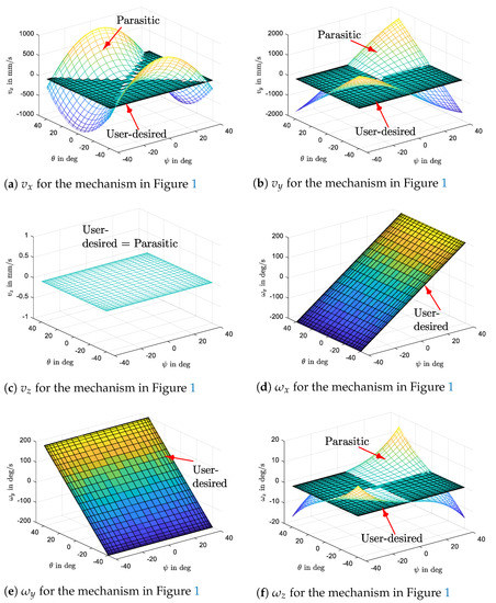
Figure 4. Numerical simulation.

Note that s and c in Equation (29) stands for sine and cosine, respectively.

From the simulation, we can see the motions that are undesired for the user but necessary for the manipulator to operate safely. Optimization should be performed to match the user’s requirements and manipulator’s specifications.

4. Optimization of Parasitic Motion

The parasitic motion has been recognized as one of the major drawbacks of the lower mobility PMs. Consecutively, several researchers have tried to eliminate it from the workspace. However, most attempts are entirely geometry dependent and applied at the position-level while most parallel manipulators control scheme is designed at the velocity-level. In this paper, the parasitic terms in the constraint-compatible velocity are optimized using the velocity-level relation derived in Section 3. From Equation (28), we can see that parasitic motions are dependent on two generic parameters, i.e., ${\omega }_x$ and ${\omega }_y$. The angles ${\xi }_i$ and ${\alpha }_i$ are simultaneously altered during the optimization procedure; the algorithm simultaneously changes the distal and proximal joint of the limbs, to determine the optimal configuration. Thus, all of them are in the vector ${\delta }_i$. i.e, ${\delta }_i={\left[\begin{array}{cc}{\xi }_i& {\alpha }_i\end{array}\right]}^T$. By denoting ${\mathit{C}}_1=\left[\begin{array}{ccc}{\mathit{v}}_0& {\mathit{v}}_1& {\mathit{v}}_2\end{array}\right]$, the inverse of ${\mathit{C}}_1$ can be rewritten in the form shown in Appendix A. Then, Equation (28) can be described in analytic form as:

$$\left[\begin{array}{c}{v}_x\\ v_y\\ {\omega }_z\end{array}\right]=\frac{1}{{\mathit{v}}_0·({\mathit{v}}_1\times {\mathit{v}}_2)}\left[\begin{array}{c}{({\mathit{v}}_1\times {\mathit{v}}_2)}^T\\ {({\mathit{v}}_2\times {\mathit{v}}_0)}^T\\ {({\mathit{v}}_0\times {\mathit{v}}_1)}^T\end{array}\right]\left[\begin{array}{cc}-a_{1z}c{\xi }_1& -a_{1z}s{\xi }_1\\ -a_{2z}c{\xi }_2& -a_{2z}s{\xi }_2\\ -a_{3z}c{\xi }_3& -a_{3z}s{\xi }_3\end{array}\right]\left[\begin{array}{c}{\omega }_x\\ {\omega }_y\end{array}\right].$$

(30)

where

$$\begin{array}{cc}\hfill {\mathit{v}}_0& ={\left[\begin{array}{ccc}c{\xi }_1& c{\xi }_2& c{\xi }_3\end{array}\right]}^T\hfill \\ \hfill {\mathit{v}}_1& ={\left[\begin{array}{ccc}-s{\xi }_1& -s{\xi }_2& -s{\xi }_3\end{array}\right]}^T\hfill \\ \hfill {\mathit{v}}_2& ={\left[\begin{array}{ccc}-(a_{1x}c{\xi }_1+a_{1y}s{\xi }_1)& -(a_{2x}c{\xi }_2+a_{2y}s{\xi }_2)& -(a_{3x}c{\xi }_3+a_{3y}s{\xi }_3)\end{array}\right]}^T.\hfill \end{array}$$

The expression for variable ${\xi }_i$ is given in Equation (4). The detail elements of the vector ${\mathit{a}}_i$ given in Equation (2) can be expanded as:

$${\mathit{a}}_i={\left[\begin{array}{ccc}{a}_{ix}& a_{iy}& a_{iz}\end{array}\right]}^T,$$

(31)

$$\begin{array}{ccc}\hfill a_{ix}& =& R_{11}{r}_{p}c{\alpha }_i+R_{12}{r}_{p}s{\alpha }_i=r_p((c\theta c\varphi +s\psi s\theta s\varphi )c{\alpha }_i+(s\psi s\theta c\varphi -c\theta s\varphi )s{\alpha }_i)\hfill \\ \hfill a_{iy}& =& R_{21}{r}_{p}c{\alpha }_i+R_{22}{r}_{p}s{\alpha }_i=r_p(c\psi s\varphi c{\alpha }_i+c\psi c\varphi s{\alpha }_i)\hfill \\ \hfill a_{iz}& =& R_{31}{r}_{p}c{\alpha }_i+R_{32}{r}_{p}s{\alpha }_i=r_p((s\psi c\theta s\varphi -s\theta c\varphi )c{\alpha }_i+(s\varphi s\theta +s\psi c\theta c\varphi )s{\alpha }_i)\hfill \end{array}$$

where ${\alpha }_i$ is the angle to locate the spherical joints from the x-axis of frame $\left\{O^{\prime }\right\}$ as in Equation (3).

Our objective in this section is to remove the parasitic motion from the workspace. Through careful observation of the parasitic motion equation, only ${\xi }_i$ and ${\alpha }_i$ are the relevant geometric parameters that can be meaningfully altered to get the configuration of the manipulator without parasitic motion. The radius $r_p$ of the moving platform does linearly relate to the parasitic motion, and from the equation, it is observed that the optimal solution is trivial, which is $r_p=0$. Thus, only angle ${\xi }_i$ and ${\alpha }_i$ will be considered as feasible design parameters and are denoted by vector ${\delta }_i$. By obtaining optimum ${\delta }_i$ for limbs 2 and 3 from the x-axis, the minimum parasitic motion can be achieved for all choices of $r_p$. Thus, the choice of $r_p$ can be left to the designers.

Subsequently, it is required to transform Equation (30) in the form that is suitable to the selected optimization algorithm. The algorithms can be single-objective such as Quasi-Newton or multi-objective such as pattern-search or Pareto-front. In this paper, the quasi-newton algorithm is used for the direction-specific optimization and the pattern search to simultaneously optimize all parasitic motions. We prefer the Quasi-Newton methods for a direction-specific optimization because it is simple and convenient when the Hessian is quite difficult to compute analytically due to system nonlinearity. For the vectorized evaluation, the pattern-search is chosen because it is a non-gradient rapid convergence algorithm for multi-objective nonlinear system. Moreover, thus solvers are valiance in Matlab optimization toolbox. For the direction-specific optimization, the x- and y-axis linear motions can be rewritten as:

$${\mathit{v}}_x=\frac{{({\mathit{v}}_1\times {\mathit{v}}_2)}^T}{{\mathit{v}}_0·({\mathit{v}}_1\times {\mathit{v}}_2)}\left[\begin{array}{cc}-a_{1z}c{\xi }_1& -a_{1z}s{\xi }_1\\ -a_{2z}c{\xi }_2& -a_{2z}s{\xi }_2\\ -a_{3z}c{\xi }_3& -a_{3z}s{\xi }_3\end{array}\right]\left\{\begin{array}{c}{\omega }_x\\ {\omega }_y\end{array}\right\},$$

(32)

and,

$${\mathit{v}}_y=\frac{{({\mathit{v}}_2\times {\mathit{v}}_0)}^T}{{\mathit{v}}_0·({\mathit{v}}_1\times {\mathit{v}}_2)}\left[\begin{array}{cc}-a_{1z}c{\xi }_1& -a_{1z}s{\xi }_1\\ -a_{2z}c{\xi }_2& -a_{2z}s{\xi }_2\\ -a_{3z}c{\xi }_3& -a_{3z}s{\xi }_3\end{array}\right]\left\{\begin{array}{c}{\omega }_x\\ {\omega }_y\end{array}\right\}.$$

(33)

To minimize the parasitic motion in a specific direction with the Equations (32) and (33) over the intended rotational workspace, the linear motion along the z-axis has no role. Moreover, it is difficult to use linear programming due to the nonlinearity of ${\mathit{C}}_1$ and ${\mathit{C}}_2$. Thus, the average $\delta v$ along the specified direction and entire rotational workspace is obtained by summing over all the columns to create a row of sums and then summing across the row to get the array’s total sum as in Equations (34) and (35).

$$\delta v_x=f(r_p,{\xi }_2,{\xi }_3,{\alpha }_2,{\alpha }_3,\psi ,\theta ,\varphi ,{\omega }_x,{\omega }_y)=\sum _{j=1}^n\sum _{k=1}^m{v}_x,$$

(34)

$$\delta v_y=f(r_p,{\xi }_2,{\xi }_3,{\alpha }_2,{\alpha }_3,\psi ,\theta ,\varphi ,{\omega }_x,{\omega }_y)=\sum _{j=1}^n\sum _{k=1}^m{v}_y.$$

(35)

Then, the Quasi-Newton algorithm is applied consecutively for Equations (34) and (35) as shown in Equation (36).

Quasi-Newton method: The quasi-Newton methods build up a curvature information at each iteration to formulate a quadratic model problem of the form:

$$\begin{array}{c}\hfill \underset{{\delta }_i}{min}\end{array}\frac{1}{2}{\delta }_i^T\mathit{H}{\delta }_i+{\mathit{g}}^T{\delta }_i+\left[f({\xi }_2,{\xi }_3,{\alpha }_2,{\alpha }_3)\right],$$

(36)

where $\mathit{H}$ is a positive definite symmetric matrix and $\mathit{g}$ is a constant vector. The condition for the optimality of Equation (36) is:

$$\nabla f\left({\delta }_i^{*}\right)=\mathit{H}{\delta }_i^{*}+\mathit{g}=0.$$

(37)

Then, the optimal solution is obtained by inverting Equation (37):

$${\delta }_i^{*}=-{\mathit{H}}^{-1}\mathit{c}.$$

(38)

Although several methods exists for updating the Hessian matrix ($\mathit{H}$) in Equation (36), Broyden–Fletcher–Goldfarb–Shanno (BFGS) is known to be effective [30]. The BFG method updates the Hessian matrix using the following relation:

$${\mathit{H}}_{k+1}={\mathit{H}}_k\frac{{\mathit{q}}_k{\mathit{q}}_k^T}{{\mathit{q}}_k^T{\mathit{q}}_k}-\frac{{\mathit{H}}_k^T{\mathit{s}}_k^T{\mathit{s}}_k{\mathit{H}}_k}{{\mathit{s}}_k^T{\mathit{H}}_k{\mathit{s}}_k},$$

(39)

where,

$$\begin{array}{cc}\hfill {\mathit{s}}_k& ={\delta }_{k+1}-{\delta }_k,\hfill \\ \hfill {\mathit{q}}_k& =\nabla f\left({\delta }_{k+1}\right)-\nabla f\left({\delta }_k\right).\hfill \end{array}$$

The inverse of $\mathit{H}$ is updated through the Davidon–Fletcher–Powell (DFP) method at each iteration [30].

At each iteration, a line search is performed in the direction:

$$\lambda =-{\mathit{H}}_k^{-1}\Delta f\left({\delta }_k\right)$$

(40)

The optimization result tells varying ${\delta }_i$ over the intended workspace, for the optimal parasitic motion, is the same result for all example manipulators used in this paper. This is demonstrated in the simulation and is shown in Figure 5a–c. Figure 5a shows the configuration of zero x-axis parasitic motion for the PhRS manipulator. Figure 5b,c shows the configuration (limb arrangement) that eliminates the x-axis parasitic motion for the PvRS and RPS manipulators, respectively. Note that the limb number convention is consistently applied for all figures and counted counterclockwise starting from the +ve x-axis throughout the paper.

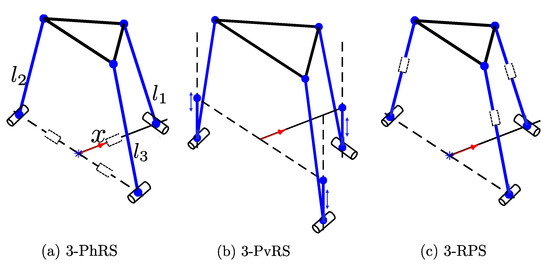
Figure 5. Optimal configuration for $v_x$ = 0.

The results shown in Figure 5 is the leg (limb) arrangement of the manipulator for zero parasitic motion along the x-axis, and these parameters are ${\xi }_1={\alpha }_1=0$${}^{\circ }$, ${\xi }_2={\alpha }_2=90$${}^{\circ }$, ${\xi }_3={\alpha }_3=-90$${}^{\circ }$. Substituting the angular values and all the corresponding elements in Equation (32) proves the result is true. Based on the result obtained, the following optimality condition can be drawn:

Conditions for $v_x=0$: To eliminate the parasitic motion along the x-axis, the center of the second and third limb’s spherical joints must be collinear, and both should be orthogonal to the first limb.

Similarly, the appropriate limb arrangement or configuration for the zero parasitic motion along the y-axis is obtained by optimizing Equation (35). Accordingly, the zero parasitic motion along this particular axis is obtained at ${\xi }_1={\alpha }_1=0$${}^{\circ }$, ${\xi }_2={\alpha }_2=90$${}^{\circ }$ and ${\xi }_3={\alpha }_3=\pm 180$${}^{\circ }$ for all three manipulators. Likewise, the following optimality condition can be drawn for $v_y=0$.

Conditions for $v_y=0$: To eliminate the parasitic motion along the y-axis, the center of the first and the third limb’s spherical joints must be collinear. i.e., ${\xi }_1=0$${}^{\circ }$, ${\xi }_2=90$${}^{\circ }$ and ${\xi }_3=\pm 180$${}^{\circ }$.

Pattern-search algorithm: Considering the Quasi-Newton algorithm is suitable only for a single-digit output objective function, the non-gradient vector optimization (multi-objective algorithm) called pattern-search is used to simultaneously optimize ${\mathit{v}}_x$ and ${\mathit{v}}_y$. The pattern-search method is a family of derivative free nonlinear numerical optimization. To reach to the optimal point, it looks a long certain specified direction, and evaluate the cost function at a given step length each of these directions. These points form a frame around the current iteration. Depending on whether any point within the pattern has a lower cost function value than the current point, the frame shrinks or expands in the next iteration. The search stops after the minimum pattern size is reached. The key condition to choose a search direction is that at least one direction in this set should give a descent direction for the cost function whenever the current point is not a stationary point.

From the sequential optimization of $v_x$ and $v_y$, we have noticed that the parasitic motion along the x- and y-axes are antagonistic functions. Therefore, the pattern-search algorithm achieved a simultaneous optimization of parasitic motions along the x- and y-axes by coinciding the center of the second limb’s spherical joint with the center of the third limb’s spherical joint, as shown in Figure 6a. Although the resulting configuration seems meaningless, it accurately tells the condition for eliminating both $v_x$ and $v_y$ parasitic motions from the workspace.

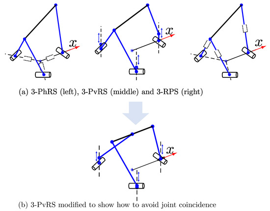
Figure 6. Optimal configuration for $v_x=v_y$ = 0.

As can be seen from Figure 6a, the limb arrangement that eliminates both parasitic motions have two coincident spherical joints. This is because of the constant length radius of the moving platform. In general, the result tells, all spherical joints need to be collinear in order for the manipulator to perform without parasitic motion. Thus, the following condition can be drawn.

Condition for $v_x=v_y=0$: To eliminate the parasitic motion in all directions, the three joints on the moving platform must be collinear. Moreover, the direction of the two revolute joints axes at the base should be parallel, while the remaining is perpendicular for both. Other example manipulators also have a similar result to that shown in Figure 6a. Thus, the example can be representative. When the two spherical joints meet at one point, as shown in Figure 6a, the design becomes complex. To avoid this problem, the radius of a limb perpendicular to the other two limbs can be adjusted to zero without loss of generality, as shown in Figure 6b. Setting $r_p=0$ for this particular limb does not violate the condition for $v_x=v_y=0$. The numerical example is provided to show these manipulators have removed the parasitic motion in the required direction. Figure 7 and Figure 8 are the task velocity for the optimal parasitic motion presented by taking the 3-RPS manipulator as a representative example.

Figure 7. v_x and v_y for the mechanism in Figure 5c.

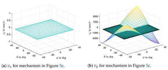
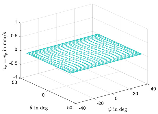
Figure 8. $v_x=v_y=0$ for mechanism arrangement in Figure 6b.

Figure 7 is the linear parasitic motion for the RPS manipulator shown in Figure 5. The simulation result shows that the x-axis parasitic motion is zero in the entire rotational workspace. Similarly, the y-axis parasitic motion is eliminated when the condition for $v_y=0$ is satisfied. Finally, the simulation for Figure 6b implies no parasitic motions in all directions. The result is shown in Figure 8. Thus, the manipulator is capable of performing pure rotation about the center of the moving plate. The resulting motion is purely spherical but with a non-spherical spatial manipulator. It is known that the rotational motion about a fixed point has usually been achieved by a spherical manipulator. Achieving a pure independent rotational motion with non-spherical spatial manipulator can improve the problems that are existed in the spherical manipulators.

During the optimization of the parasitic motion, two types of optimal structures are obtained, i.e., direction-specific optimal manipulator and manipulators with zero parasitic motion in all directions. Depending on the desired application, the direction-specific optimal manipulator can be chosen. For example, suppose the task strictly requires zero parasitic motion along the x-axis but loosens-up sensitivity for the y-parasitic motion. In that case, the result shown in Figure 5 can be used. Likewise, when the x-axis parasitic motion is not critical, the manipulator with the zero parasitic motion along the y-axis can be used.

5. Performance Evaluation of Optimal Manipulator Designs

It is necessary to evaluate these optimized manipulators’ performance within their rotational workspace to make sure the resulted optimal manipulators are usable. A dimensionally homogeneous Jacobian method is used to evaluate the performance of these manipulators [31]. Interested readers can get the detailed derivation procedure in the reference paper. For the dimensionally homogeneous Jacobian, the manipulator actuation wrenches are obtained using the same procedure as that of the constraints. Taking the 3-RPS manipulator as a representative example for consistency, Figure 9 depicts the manipulability-based performance simulation for the manipulator that removes x-axis parasitic motion. We can see that the performance of the manipulator shown in Figure 5c is dropped or not very close to one. Note that the manipulator performs well when the manipulability index is one or close to one [32]. Moreover, the manipulability evaluation of optimal design exhibits poor performance as shown in Figure 6. The simulation is not provided because the property can be seen from Figure 6. Thus, the manipulator is singular and has lost a rotational DoF about the x-axis. This is because of the location center of the spherical joint of the second limb.

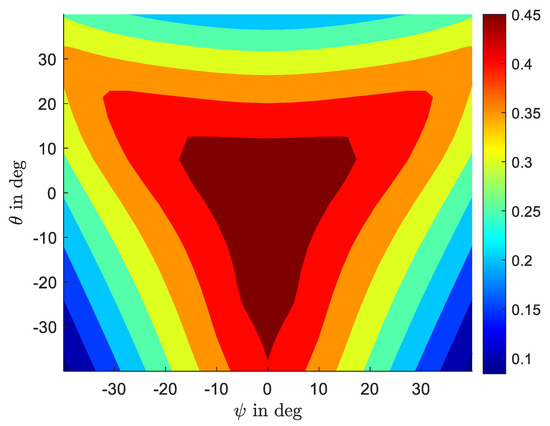
Figure 9. Manipulability of PhRS Figure 5c where parasitic motion along x-axis is removed.

The optimal conditions are only related to the collinearity of rotational center of joints on the moving plate and limb arrangements as discussed in previous sections. Thus, the remedy to enhance the performance of the manipulator without changing the mechanism motion property and optimality conditions can be done by creating a special geometric arrangement to the spherical joint of the particular limb. As can be seen from Figure 10, the spherical joint of the second limb is decoupled to a revolute-universal layout. Hence, the revolute joint near the moving platform will help the manipulator escape the singularity and improve the manipulator’s performance eventually. The following section analyzes the kinematics and performance of the modified manipulator.

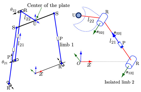
Figure 10. Non-Parasitic motion enhanced performance manipulators (left). Isolated limb (right).

Jacobian of the Limb with Decoupled Joint

For the manipulators shown in Figure 10, the motion of the limb with the decoupled joint is generated by a $4{\$}_0-1{\$}_{\infty }$ screws. Taking the center of the second revolute joint as a reference point, the direction vector of the restriction screw for the limb shown in Figure 10 can be obtained from a five system as:

$$\begin{array}{c}\hfill {\mathit{s}}_{c{12}_{\Vert }}=-[{\mathit{s}}_{{52}_{\Vert }}·({\mathit{s}}_{{32}_{\Vert }}\times {\mathit{s}}_{{12}_{\Vert }})]\left({\mathit{r}}_{54}\times {\mathit{s}}_{{42}_{\Vert }}\right)\times {\mathit{s}}_{{22}_{\Vert }}\\ \hfill +[{\mathit{s}}_{{52}_{\Vert }}·({\mathit{s}}_{{42}_{\Vert }}\times {\mathit{s}}_{{12}_{\Vert }})]\left({\mathit{r}}_{53}\times {\mathit{s}}_{{32}_{\Vert }}\right)\times {\mathit{s}}_{{22}_{\Vert }}\\ \hfill -[{\mathit{s}}_{{52}_{\Vert }}·({\mathit{s}}_{{42}_{\Vert }}\times {\mathit{s}}_{{32}_{\Vert }})]\left({\mathit{r}}_{52}\times {\mathit{s}}_{{12}_{\Vert }}\right)\times {\mathit{s}}_{{22}_{\Vert }}.\end{array}$$

(41)

Because ${\mathit{r}}_{54}=0$, the direction vector in Equation (41) can be simplified to:

$$\begin{array}{c}\hfill {\mathit{s}}_{c{12}_{\Vert }}=+[{\mathit{s}}_{{52}_{\Vert }}·(s_{{42}_{\Vert }}\times {\mathit{s}}_{{12}_{\Vert }})]\left({\mathit{r}}_{53}\times s_{{32}_{\Vert }}\right)\times {\mathit{s}}_{{22}_{\Vert }}\\ \hfill -[{\mathit{s}}_{{52}_{\Vert }}·({\mathit{s}}_{{42}_{\Vert }}\times {\mathit{s}}_{{32}_{\Vert }})]\left({\mathit{r}}_{52}\times {\mathit{s}}_{{12}_{\Vert }}\right)\times {\mathit{s}}_{{22}_{\Vert }}.\end{array}$$

(42)

With the condition of linear independence of ${\mathit{s}}_{32\Vert },{\mathit{s}}_{42\Vert },{\mathit{s}}_{52\Vert }$, the moment vector is zero. Then, the second limb restriction screw becomes:

$${\$}_{c12}={\left[\begin{array}{cc}\mathbf{0}& {\mathit{s}}_{c12\Vert }\end{array}\right]}^T,$$

(43)

where ${\mathit{s}}_{c12\Vert }={\mathit{s}}_{32\Vert }({\mathit{r}}_{53}·{\mathit{s}}_{22\Vert })+{\mathit{s}}_{12\Vert }({\mathit{r}}_{52}·{\mathit{s}}_{22\Vert })$. Note that ${\mathit{r}}_{53}={\mathit{l}}_{22}$ and ${\mathit{r}}_{52}={\mathit{l}}_{21}+{\mathit{l}}_{22}$.

From further simplification of the restriction screw, we can see vector ${\mathit{s}}_{c12\Vert }$ is parallel to ${\mathit{s}}_{12\Vert }$. By transforming the reference point and taking the constraint wrench of all three legs, we obtain the constraint matrix. Then, with the extended Jacobian, we obtain the first revolute joint wrench can be obtained from:

$$\left[\begin{array}{cc}{\mathit{s}}_{52\Vert }^T& {({\mathit{s}}_{52\Vert }\times {\mathit{l}}_{22})}^T\\ {\mathit{s}}_{42\Vert }^T& {({\mathit{s}}_{42\Vert }\times {\mathit{l}}_{22})}^T\\ {\mathit{s}}_{32\Vert }& \mathbf{0}\\ {\mathbf{0}}^T& {\mathit{s}}_{22\Vert }^T\\ \mathbf{0}& {\mathit{s}}_{c12\Vert }^T\end{array}\right]\left[\begin{array}{c}{\mathit{w}}_{p12\perp }\\ {\mathit{w}}_{p12\Vert }\end{array}\right]=\mathbf{0}:3{\$}_0-2{\$}_{\infty }.$$

(44)

For Equation (44), the direction vector is simultaneously orthogonal to ${\mathit{s}}_{21}$ and ${\mathit{s}}_{c12\Vert }$. Therefore, ${\mathit{w}}_{p12\Vert }={\mathit{s}}_{22}\times {\mathit{s}}_{c12\Vert }$. The moment vector is obtained from Equation (44), and thus ${\mathit{w}}_{p12\perp }={\mathit{M}}_1^{†}{\mathit{M}}_2{\mathit{w}}_{p12\Vert }$, where ${\mathit{M}}_1$ and ${\mathit{M}}_2$ are matrices spanned by the set of direction and moment vectors of Equation (44), respectively. The active (prismatic) joint wrench is also obtained from the following constraint equation:

$$\left[\begin{array}{cc}{\mathit{s}}_{52\Vert }^T& {({\mathit{s}}_{52\Vert }\times {\mathit{l}}_{22})}^T\\ {\mathit{s}}_{42\Vert }^T& {({\mathit{s}}_{42\Vert }\times {\mathit{l}}_{22})}^T\\ {\mathit{s}}_{32\Vert }& \mathbf{0}\\ {\mathit{s}}_{12\Vert }^T& {({\mathit{s}}_{12\Vert }\times {\mathit{l}}_{21})}^T\\ \mathbf{0}& {\mathit{s}}_{c12\Vert }^T\end{array}\right]\left[\begin{array}{c}{\mathit{w}}_{a22\perp }\\ {\mathit{w}}_{a22\Vert }\end{array}\right]=\mathbf{0}.$$

(45)

Since, ${\mathit{s}}_{c12\Vert }\Vert {\mathit{s}}_{22\Vert }$, the direction vector of active wrench becomes:

$${\mathit{w}}_{a22\Vert }=-{\mathit{r}}_{53}({\mathit{s}}_{32\Vert }·{\mathit{s}}_{c12\Vert })-{\mathit{r}}_{52}({\mathit{s}}_{12\Vert }·{\mathit{s}}_{c12\Vert }).$$

(46)

Similarly, the third joint (revolute) wrench is obtained from:

$$\left[\begin{array}{cc}{\mathit{s}}_{52\Vert }^T& {({\mathit{s}}_{52\Vert }\times {\mathit{l}}_{22})}^T\\ {\mathit{s}}_{42\Vert }^T& {({\mathit{s}}_{42\Vert }\times {\mathit{l}}_{22})}^T\\ {\mathit{s}}_{12\Vert }^T& {({\mathit{s}}_{12\Vert }\times {\mathit{l}}_{21})}^T\\ {\mathbf{0}}^T& {\mathit{s}}_{22\Vert }^T\\ \mathbf{0}& {\mathit{s}}_{c12\Vert }^T\end{array}\right]\left[\begin{array}{c}{\mathit{w}}_{p32\perp }\\ {\mathit{w}}_{p32\Vert }\end{array}\right]=\mathbf{0}:3{\$}_0-2{\$}_{\infty }.$$

(47)

Then, the direction vector becomes:

$${\mathit{w}}_{p32\Vert }={\mathit{s}}_{22\Vert }\times {\mathit{s}}_{c12\Vert }.$$

(48)

The first three rows are independent. So, the moment vector is zero. Finally, the reference point is converted to the center of the moving platform by the following transformation matrix, and all screws are related to frame $\left\{O^{\prime }\right\}$ to represent the manipulator.

$$\left[\begin{array}{cc}\mathit{I}& \mathbf{0}\\ [{\mathit{l}}_{22}{]}_{\times }& \mathit{I}\end{array}\right]$$

(49)

where ${\mathit{l}}_{22}$ is the vector representing the second link of the second limb. Generally, the inverse Jacobian of the mechanism has a dimension of $10\times 6$ consisting of 3 active joint wrenches, 4 passive joint wrenches, and 3 constraints. However, for performance analysis, the passive joint wrench is not required.

With the rearranged spherical joint of one limb, the parasitic motion of the manipulator is eliminated without entering a singular configuration. For this manipulator, the fastest way to analytically prove there is no parasitic motion is to compute the center position of the moving platform from the constraint in Equation (50).

$${(\mathit{p}+\mathit{R}{\mathit{a}}^{\prime }i)}^T{\mathit{s}}_{i2\Vert }=0$$

(50)

where

$$\begin{array}{c}\hfill \mathit{p}={\left[\begin{array}{ccc}x& y& z\end{array}\right]}^T,a_1^{\prime }={\left[\begin{array}{ccc}{r}_p& 0& 0\end{array}\right]}^T,a_2^{\prime }={\left[\begin{array}{ccc}0& 0& 0\end{array}\right]}^T,a_3^{\prime }={\left[\begin{array}{ccc}0& 0& r_p\end{array}\right]}^T,\\ \hfill {\mathit{s}}_{11\Vert }{\left[\begin{array}{ccc}0& 1& 0\end{array}\right]}^T,{\mathit{s}}_{12\Vert }{\left[\begin{array}{ccc}1& 0& 0\end{array}\right]}^T,{\mathit{s}}_{22\Vert }{\left[\begin{array}{ccc}1& 0& 0\end{array}\right]}^T,{\mathit{s}}_{13\Vert }{\left[\begin{array}{ccc}-1& 0& 0\end{array}\right]}^T.\end{array}$$

(51)

Substituting Equation (51) into Equation (50) gives:

$$\begin{array}{c}\hfill {(\mathit{p}+\mathit{R}{\mathit{a}}^{\prime }1)}^T{\mathit{s}}_{11\Vert }=y+R_{21}{r}_p=0,\end{array}$$

(52)

$$\begin{array}{c}\hfill {(\mathit{p}+\mathit{R}{\mathit{a}}^{\prime }2)}^T{\mathit{s}}_{12\Vert }={(\mathit{p}+\mathit{R}{\mathit{a}}^{\prime }2)}^T{\mathit{s}}_{22\Vert }=x+R{a}_2^{\prime }=0,\end{array}$$

(53)

$$\begin{array}{c}\hfill {(\mathit{p}+\mathit{R}{\mathit{a}}^{\prime }3)}^T{\mathit{s}}_{13\Vert }=y+R_{21}{r}_p=0,\end{array}$$

(54)

From Equations (52) and (54), we know $y=\varphi =0$, and from Equation (53) we know $x=0$. Similarly, substituting Equation (51) into Equation (28) produces no parasitic velocity.

Then, the performance of the manipulators is evaluated by applying the method presented in [31]. Figure 11 shows that the manipulator’s manipulability index is close to 1 at the central region of the moving platform. The performance drops near the boundary of orientational workspace as expected.

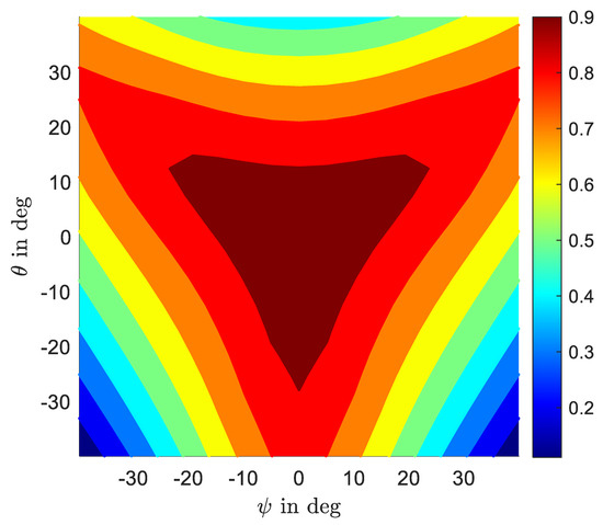
Figure 11. Manipulablity of the design shown in Figure 10 when $v_x$=$v_y$ = 0.

From the result, we can clearly see that the performance of the manipulator is enhanced, and the parasitic motions have vanished from the workspace. To conclude, this section utilized the velocity-level analytic coupling relation to get the optimal manipulator. The performance evaluation is performed, and an enhanced performance manipulator is presented.

6. Conclusions

This paper studied a velocity-level approach to formulate and optimize parasitic motion. First, the structural constraint is embedded in the motion equation utilizing the reciprocal screw method. Then, the coupling relationship between the independent and parasitic terms is formulated from the analytic velocity constraint. From the coupling equation, we identified the terms that cause the parasitic motion. Thus, the relevant design variables are isolated for optimization. By directly formulating the cost function from the screw-based velocity constraint, the velocity-level optimization is performed, and parasitic motions are removed. For implementation, Matlab Optimization Toolbox™ is used. The performance evaluation is conducted to ensure the usefulness of the optimal manipulator. However, the evaluation result showed that the optimized manipulator has low performance. Because the optimal configuration is achieved by changing the location of the limbs to a non-uniform pattern around the fixed frame’s z-axis and, the joints on the moving platform should be collinear to remove parasitic motion entirely from the workspace. Thus, the load on the moving plate cannot equally distribute to all legs. Also, the collinearity of the joints transformed the platform into a line that may not perfectly perform all required DoFs. These features of the manipulator eventually lead to poor performance if not a singularity. One of the leg’s spherical joints is rearranged to a special scheme to overcome this issue. Then, the performance is adequately improved. This procedure is uniformly applied to other example manipulators and has shown the same outcome. Therefore, the results of other manipulators are not included in the paper to avoid redundancy. Manipulators that do not have any parasitic motion are easy to control with enhanced accuracy. Therefore, it can be used for applications that are sensitive to parasitic movement.

References

- Zhou, C.C.; Fang, Y.F. Design and analysis for a three-rotational-dof flight simulator of fighter-aircraft. Chin. J. Mech. Eng. (Engl. Ed.) 2018, 31, 55. [Google Scholar] [CrossRef]
- Tanev, T.K. Minimally-invasive-surgery parallel robot with non-identical limbs. In Proceedings of the 2014 IEEE/ASME 10th International Conference on Mechatronic and Embedded Systems and Applications (MESA), Senigallia, Italy, 10–12 September 2014; pp. 1–6. [Google Scholar] [CrossRef]
- Wang, M.; Liu, H.; Huang, T.; Chetwynd, D.G. Compliance analysis of a 3-SPR parallel mechanism with consideration of gravity. Mech. Mach. Theory 2015, 84, 99–112. [Google Scholar] [CrossRef]
- Miermeister, P.; Lächele, M.; Boss, R.; Masone, C.; Schenk, C.; Tesch, J.; Kerger, M.; Teufel, H.; Pott, A.; Bülthoff, H.H. The CableRobot simulator large scale motion platform based on Cable Robot technology. In Proceedings of the IEEE International Conference on Intelligent Robots and Systems, Daejeon, Korea, 9–14 October 2016; pp. 3024–3029. [Google Scholar] [CrossRef]
- Pisla, D.; Plitea, N.; Gherman, B.; Pisla, A.; Vaida, C. Kinematical analysis and design of a new surgical parallel robot. In Proceedings of the 5th International Workshop on Computational Kinematics, Duisburg, Germany, 6–8 May 2009; pp. 273–282. [Google Scholar] [CrossRef]
- Kuo, C.H.; Dai, J.S.; Dasgupta, P. Kinematic design considerations for minimally invasive surgical robots: An overview. Int. J. Med. Robot. Comput. Assist. Surg. 2012, 8, 127–145. [Google Scholar] [CrossRef] [PubMed]
- Jones, T.P. Kinematics, Dynamics and Design of a Spherical Positioning Robot for Satellite Tracking and Other Applications. Ph.D. Thesis, University of Canterbury, Christchurch, New Zealand, 1996. [Google Scholar] [CrossRef]
- Yu, Y.; Xu, Z.B.; Han, C.Y.; Han, H.; Wang, X.M.; Wu, Q.W. Design and testing of parallel alignment mechanism for space optical payload. In Proceedings of the 2017 2nd Asia-Pacific Conference on Intelligent Robot Systems, ACIRS, Wuhan, China, 16–18 June 2017; pp. 254–258. [Google Scholar] [CrossRef]
- Gressler, W.J. LSST telescope and site status. In Ground-Based and Airborne Telescopes VI; Hall, H.J., Gilmozzi, R., Marshall, H.K., Eds.; International Society for Optics and Photonics, SPIE: Edinburgh, UK, 2016; Volume 9906, pp. 175–189. [Google Scholar] [CrossRef]
- Jáuregui, J.C.; Hernández, E.E.; Ceccarelli, M.; López-Cajún, C.; García, A. Kinematic calibration of precise 6-DOF Stewart platform-type positioning systems for radio telescope applications. Front. Mech. Eng. 2013, 8, 252–260. [Google Scholar] [CrossRef]
- Sun, J.; Shao, L.; Fu, L.; Han, X.; Li, S. Kinematic analysis and optimal design of a novel parallel pointing mechanism. Aerosp. Sci. Technol. 2020, 104, 105931. [Google Scholar] [CrossRef]
- Carretero, J.A.; Podhorodeski, R.P.; Nahon, M.A.; Gosselin, C.M. Kinematic analysis and optimization of a new three degree-of-freedom spatial parallel manipulator. J. Mech. Des. Trans. ASME 2000, 122, 17–24. [Google Scholar] [CrossRef]
- Bernabe, L.; Raynal, N.; Michel, Y. 3Pod: A High Performance Parallel Antenna Pointing Mechanism. In Proceedings of the 15th European Space Mechanisms & Tribology Symposium—ESMATS 2013’, Noordwijk, The Netherlands, 25–27 September 2013; pp. 25–27. [Google Scholar]
- Itul, T.; Pisla, D. Dynamics of a 3-DOF parallel mechanism used for orientation applications. In Proceedings of the 2008 IEEE International Conference on Automation, Quality and Testing, Robotics, AQTR 2008—THETA 16th Edition, Cluj-Napoca, Romania, 22–25 May 2008; Volume 2, pp. 398–403. [Google Scholar] [CrossRef]
- Starrag Group Receives Large Order in the US-Orizon. 2016. Available online: https://www.orizonaero.com/news/single/starrag-group-receives-large-order-us/ (accessed on 5 May 2021).
- Huang, T.; Liu, H. Parallel Mechanism Having Two Rotational and One Translational Degrees of Freedom. U.S. Patent US7793564, 14 September 2010. [Google Scholar]
- Chen, G.; Yu, W.; Li, Q.; Wang, H. Dynamic modeling and performance analysis of the 3-PRRU 1T2R parallel manipulator without parasitic motion. Nonlinear Dyn. 2017, 90, 339–353. [Google Scholar] [CrossRef]
- Li, Y.G.; Liu, H.T.; Zhao, X.M.; Huang, T.; Chetwynd, D.G. Design of a 3-DOF PKM module for large structural component machining. Mech. Mach. Theory 2010, 45, 941–954. [Google Scholar] [CrossRef]
- Hennes, N. Ecospeed—An innovative machinery concept for high performance 5 axis machining of large structural components in aircraft engineering. In Proceedings of the 3rd Chemnitz Parallel Kinematic Seminar, Caldes de Malavella, Spain, 24–28 June 2002; pp. 763–774. [Google Scholar]
- Tanev, T.K.; Cammarata, A.; Marano, D.; Sinatra, R. Elastostatic model of a new hybrid minimally-invasive-surgery robot. In Proceedings of the 2015 IFToMM World Congress (IFToMM 2015), Taipei, Taiwan, 25–30 October 2015. [Google Scholar] [CrossRef]
- Yaşır, A.; Kiper, G.; Dede, M.C. Kinematic design of a non-parasitic 2R1T parallel mechanism with remote center of motion to be used in minimally invasive surgery applications. Mech. Mach. Theory 2020, 153, 104013. [Google Scholar] [CrossRef]
- Li, Q.; Chen, Z.; Chen, Q.; Wu, C.; Hu, X. Parasitic motion comparison of 3-PRS parallel mechanism with different limb arrangements. Robot. Comput.-Integr. Manuf. 2011, 27, 389–396. [Google Scholar] [CrossRef]
- Qu, H.; Fang, Y.; Guo, S. Parasitic rotation evaluation and avoidance of 3-UPU parallel mechanism. Front. Mech. Eng. 2012. [Google Scholar] [CrossRef]
- Liu, X.; Wu, C.; Wang, J.; Bonev, I. Attitude description method of [PP]S type parallel robotic mechanisms. Jixie Gongcheng Xuebao/Chin. J. Mech. Eng. 2008, 44, 19–23. [Google Scholar] [CrossRef]
- Kim, D.; Chung, W.K. Analytic formulation of reciprocal screws and its application to nonredundant robot manipulators. J. Mech. Des. Trans. ASME 2003, 125, 158–164. [Google Scholar] [CrossRef]
- Kim, D. Kinematic Analysis of Spatial Parallel Manipulators: Analytic Approach with the Restriction Space. Ph.D. Thesis, Pohang University of Science and Technology, Pohang, Korea, 2002. [Google Scholar]
- Kim, D.; Chung, W.; Youm, Y. Analytic Jacobian of in-parallel manipulators. In Proceedings of the 2000 ICRA, Millennium Conference, IEEE International Conference on Robotics and Automation. Symposia Proceedings (Cat. No.00CH37065), San Francisco, CA, USA, 24–28 April 2000; Volume 3, pp. 2376–2381. [Google Scholar] [CrossRef]
- Lipkin, H.; Duffy, J. The Elliptic Polarity of Screws. J. Mech. Transm. Autom. Des. 1985, 107, 377–386. [Google Scholar] [CrossRef]
- Nigatu, H.; Yihun, Y. Algebraic Insight on the Concomitant Motion of 3RPS and 3PRS PKMs. Mech. Mach. Sci. 2020, 83, 242–252. [Google Scholar] [CrossRef]
- Jorge Nocedal, S.J.W. Numerical Optimization; Springer Series in Operations Research and Financial Engineering; Springer: New York, NY, USA, 2006. [Google Scholar] [CrossRef]
- Liu, H.; Huang, T.; Chetwynd, D.G. A Method to Formulate a Dimensionally Homogeneous Jacobian of Parallel Manipulators. IEEE Trans. Robot. 2011, 27, 150–156. [Google Scholar] [CrossRef]
- Merlet, J.P. Jacobian, manipulability, condition number, and accuracy of parallel robots. J. Mech. Des. Trans. ASME 2006, 128, 199–206. [Google Scholar] [CrossRef]
Publisher’s Note: MDPI stays neutral with regard to jurisdictional claims in published maps and institutional affiliations. |
© 2021 by the authors. Licensee MDPI, Basel, Switzerland. This article is an open access article distributed under the terms and conditions of the Creative Commons Attribution (CC BY) license (https://creativecommons.org/licenses/by/4.0/).