Dynamic Maneuverability Analysis: A Preliminary Application on an Autonomous Underwater Reconfigurable Vehicle

Abstract

Since the development of the first autonomous underwater vehicles, the demanded tasks for subsea operations have become more and more challenging as, for instance, intervention, maintenance and repair of seabed installations, in addition to surveys. As a result, the development of autonomous underwater reconfigurable vehicles (AURVs) with the capability of interacting with the surrounding environment and autonomously changing the configuration, according to the task at hand, can represent a real breakthrough in underwater system technologies. Driven by these considerations, an innovative AURV has been designed by the Department of Industrial Engineering of the University of Florence (named as UNIFI DIEF AURV), capable of efficiently reconfiguring its shape according to the task at hand. In particular, the UNIFI DIEF AURV has been provided with two extreme configurations: a slender (“survey”) configuration for long navigation tasks, and a stocky (“hovering”) configuration designed for challenging goals as intervention operations. In order to observe the several dynamic features for the two different configurations, a novel formulation for the dynamic maneuverability analysis (DMA) of an AURV, adapting Yoshikawa’s well-known manipulability theory for robotic arms, is proposed in this work. More specifically, we introduce a novel analysis which relates the vehicle body-fixed accelerations with the rotational speed of each thruster, taking into account also the AURV dynamic model for each configuration and the propulsion system.

1. Introduction

The off-shore oil and gas industry has a growing demand for new and innovative solutions for inspection, maintenance and repair of seabed installations. Currently, these tasks are usually carried out in hostile environments using remotely operated vehicles (ROVs) deployed from a large surface vessel; however, ROV operations require high expenses due to the daily ship cost and the large number of crew members which such operations need. As a result, in order to reduce the inspection cost and deal with the several logistic constraints, the interest in autonomous underwater vehicles (AUVs) has rapidly increased in the last few years. Indeed, AUVs are currently exploited for long-distance monitoring and inspection, as they are provided with an ever-increasing precision navigation system [1,2]. Moreover, the development of vehicles that can incorporate both the AUV inspection and ROV intervention functionalities is one of the most challenging tasks of the underwater industry as well as the scientific community [3]. A recent example is Hydrone-R, the underwater intervention drone (UID) from Saipem S.p.A., which is a technology that allows accurate inspections on submarine systems, certifies operation, and detects and prevent any malfunctions [4]. With the regard of other innovative AUVs, the basic idea concerns vehicle with many configurations and the ability to autonomously switch between them depending on the main task to accomplish. For instance, the autonomous underwater reconfigurable vehicles (AURV) can select the most appropriate configuration so as to dive with the optimal fluid dynamic efficiency and achieve the minimum power consumption for long distance navigation; furthermore, the robot may be provided with a larger number of degrees of freedom for complex manipulation operations or to perform autonomous docking in a subsea station. As a matter of fact, AURVs do arise as a promising tool for incorporating several reconfigurable modules and accomplishing both the autonomous navigation/inspection and intervention tasks.

As far as the AURV state of the art is concerned, one of the most innovative vehicles is made by EELUME [5,6], an underwater snake robot (USR), developed by Subsea Intervention for underwater inspection and manipulation. This vehicle is basically a self-propelled robotic arm that can move over long distances and carry out maintenance and repair tasks in spaces not usually accessible by conventional underwater vehicles. In greater detail, it is a modular, flexible robot capable of swimming like a snake, or being propelled by conventional thrusters. Additionally, the vehicle can be assembled with an arbitrary number of elements linked each other with a flexible joint. Another example of AURV has been presented by Houston Mechatronics in 2018; specifically, Houston Mechatronics is a subsea service company with deep expertise in robotics and intelligent automation, founded by former NASA roboticists responsible for designing and developing some of the most advanced robots in the world. 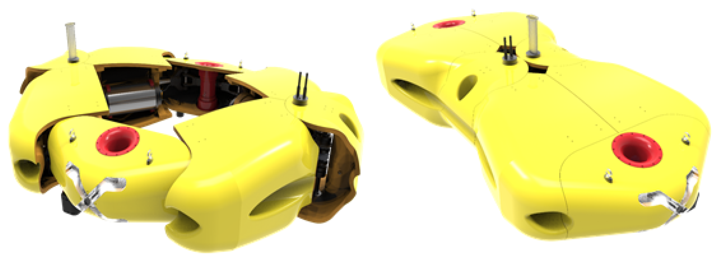The conceptual vehicle, named Aquanaut [7], is a robot with two different configurations: in AUV mode, it can cover long distances while accomplishing tasks like seabed mapping, and inspection of large area; in ROV mode, the hull can open its structure, exposing two robotic arms for manipulation operations. In particular, in the closed version, the vehicle appears as a classical UUV with a slender shape; in this configuration, it can move itself with only three motors for long distance, controlling only three degrees of freedoms. In the open version, the upper part of the hull moves away from the main body, exposing other four motors, in order to obtain a vectored configuration of the motors, and two robotics arms. Driven by these considerations, an innovative AURV [8,9], capable of efficiently reconfiguring its shape, according to the demanded task, spanning from a “survey”, slender configuration to a “hovering”, stocky configuration have been designed by the Department of Industrial Engineering of the University of Florence (UNIFI DIEF). After the design stage has been partially fulfilled, the need for investigating the dynamic characteristics of the two different extreme configurations has arisen. In fact, a novel formulation for the dynamic maneuverability analysis (DMA) of an AURV, adapting Yoshikawa’s well-known manipulability theory for robotic arms [10,11], is proposed in this paper. If the manipulability concept was first introduced as a measure of the ability of robotic arms in positioning and orienting end effectors, in the same way, the maneuverability can be defined as the capability of a mobile robot to move over several degrees of freedom. With regard to the application of the maneuverability concept in subsea robotics, several works [12,13] discussed the optimization of thruster configurations for omnidirectional underwater vehicles. In particular, the relationship between the longitudinal forces of the thrusters and the body-fixed generalized forces has been studied. In the context of our work, we are not only introducing a novel analysis that relates the vehicle body-fixed accelerations with the rotational speed of each thruster, but we apply this methodology to several AURV configurations. Furthermore, we provide an accurate description of the AURV dynamic model and the propulsion system for each vehicle configuration.

The paper structure reflects the procedural workflow. In Section 2, we summarize the research activity design guidelines alongside a review of the major exploited theoretical concepts. In Section 3, we briefly illustrate the kinematic and dynamic behavior of each configuration of the AURV with the assumptions made in this work. In Section 4, we provide the study of the propulsion system selected for the vehicle. Additionally, in Section 5, we describe the new dynamic maneuverability formulation, starting from the theoretical basics, to the application of this theory to an underwater vehicle. In Section 6, we outline the metrics and indices used for a quantitative evaluation of the AURV maneuverability. Finally, the simulation results of the DMA applied to the UNIFI DIEF AURV can be observed in Section 7. A conclusive discussion is provided in Section 8.

2. The UNIFI DIEF AURV

As highlighted in Section 1, AURVs can be the key to push the boundaries of the underwater robotics technologies by merging the robot capabilities of performing both the surveys and inspection/intervention tasks by maintaining high-standard effectiveness and efficiency. As a consequence, we have designed an innovative AURV (Figure 1) capable of efficiently reconfiguring its shape, spanning from a “survey”, slender configuration to a “hovering”, stocky configuration [9]. This innovative solution allows switching between a stocky and symmetrical shape, with an isotropic behavior useful to face unexpected external disturbances (e.g., marine currents and water flow induced by waves is the vehicle is at low depth), and a slender one, with an elongated body to minimize the hydrodynamic drag (i.e., reducing the power consumption) in the longitudinal direction.

Nevertheless, the major benefit is not limited to a hydrodynamic shape variation; the vehicle is furtherly supplied with the key ability to change its geometrical structure and, then, its motors configuration. By analyzing the propulsion layouts, the UNIFI DIEF AURV configuration is an eight thruster arrangement with four of them fixed on the horizontal plane and four thrusters on the vertical direction in the body-fixed frame. In particular, the hovering configuration has a perfect vectored layout in the horizontal plane, with the ability of a fully $3D$ motion, while in the survey configuration the horizontal thrusters result aligned, thus maximizing the thrust in the longitudinal direction of motion. Finally, the aforementioned “shape changing ability” is guaranteed by two distinct types of joint (Figure 2): two actuated and four free joints.

A more comprehensive overview of the technical features concerning the UNIFI DIEF AURV was illustrated in a previous work of the authors [8]. An exhaustive discussion of the vehicle mechanical layout was reported there.

3. Kinematic and Dynamic Modeling for AURVs

The kinematic and dynamic description of the UNIFI DIEF AURV is briefly discussed in this Section; for the sake of completeness, the two different and extreme vehicle configurations have been studied in a decoupled manner, without the development of a multibody model [14,15] (whose development is, nonetheless, planned as a strategic solution for future research activities). In light of these considerations, the kinematic models, commonly exploited for AUVs by the scientific community [16,17], have been employed for both the hovering and survey configurations. To be more specific, in the following, we assume that once one of the two extreme configurations, described by the joint coordinate vector $\mathit{q}$, has been reached, it does not change dynamically and the reconfigurable vehicle can be considered as a unique rigid body.

Within the context of this work, the following notation is employed: a generic vector $\mathit{p}\in {\mathbb{R}}^3$ expressed in a particular $\left\{O^0{x}^0{y}^0{z}^0\right\}$ frame is denoted with ${}^0\mathit{p}$, whereas, if it is convenient to define vectors without an explicit reference to a specific coordinate frame (coordinate free vector), it will be simply indicated with $\mathit{p}$. A generic rotation matrix $R\in \mathbb{SO}\left(3\right)$ is indicated with two indices $R_i^j$, where the notation represents the unit vectors of the frame i with respect to frame j. 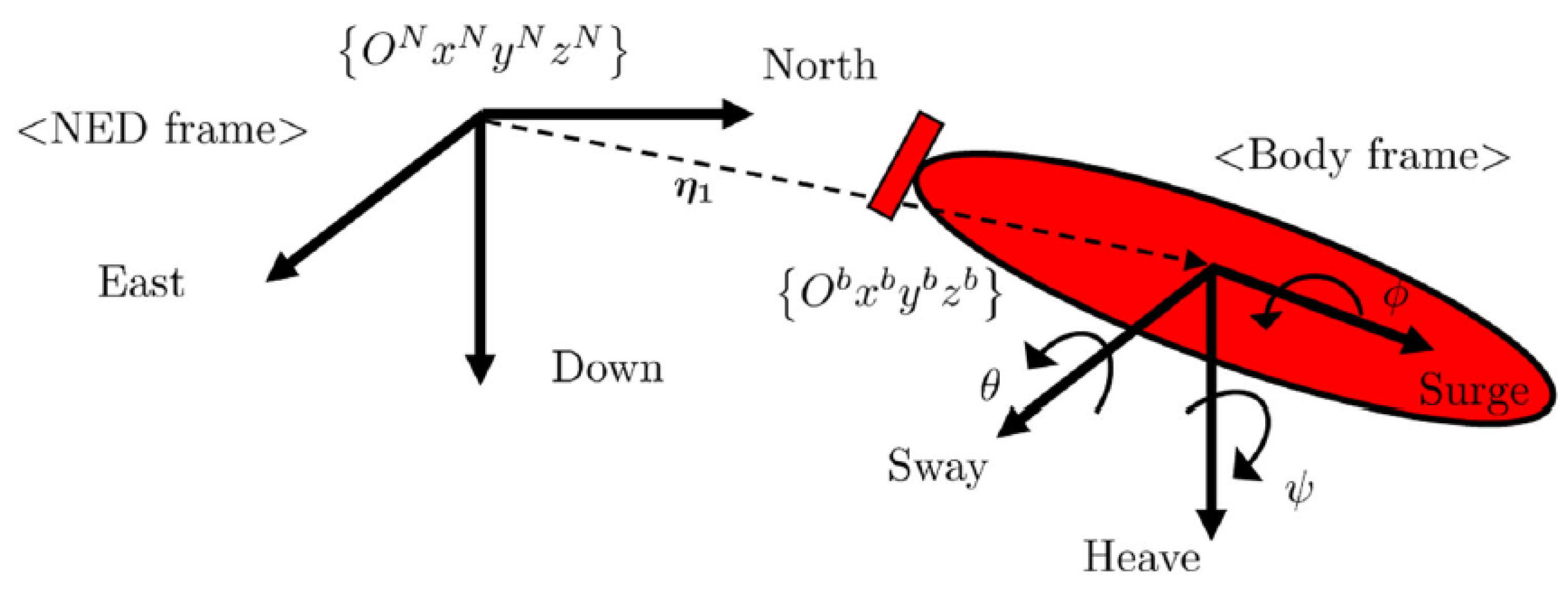Following the Society of Naval Architects and Marine Engineers (SNAME) notation [16], the state of an underwater vehicle (considered as a rigid body) is represented by using two reference frames. A local Earth-fixed reference frame (hypothesized as inertial) with axes pointing north, east, and down (NED frame) $\left\{O^N{x}^N{y}^N{z}^N\right\}$, and a right-handed body reference frame $\left\{O^b{x}^b{y}^b{z}^b\right\}$ whose origin is the center of mass of the vehicle (see Figure 3) with its x-axis pointing in the forward motion direction, its z-axis pointing down, and its y-axis completing a right-handed reference frame. The pose of a vehicle is therefore represented with

$$\mathit{\eta }={\left[{}^N{\mathit{\eta }}_1{\mathit{\eta }}_2\right]}^{\top },$$

(1)

where ${}^N{\mathit{\eta }}_1$ is the position of $O^b$ with respect to the NED frame, and ${\mathit{\eta }}_2$ is the orientation the body-fixed frame w.r.t. the NED frame, where roll ($\varphi$), pitch ($\theta$), and yaw ($\psi$) (RPY) angles are employed to describe the orientation. Additionally, AUV linear and angular velocities along the axis of the body-fixed reference (surge, sway, and heave motion) can be denoted as

$$\mathit{\nu }{=}^b\mathit{\nu }={\left[{}^b{\mathit{\nu }}_1{}^b{\mathit{\nu }}_2\right]}^{\top }.$$

(2)

The differential kinematic model is shown in Equation (3), and further information can be found in [17].

$$\begin{array}{c}\dot{\mathit{\eta }}=J\left(\mathit{\eta }\right)\mathit{\nu }\\ \left(\begin{array}{c}\hfill {}^N{\dot{\mathit{\eta }}}_1\\ \hfill {\dot{\mathit{\eta }}}_2\end{array}\right)=\left[\begin{array}{cc}{R}_b^N\left({\mathit{\eta }}_2\right)\hfill & 0_{3\times 3}\hfill \\ 0_{3\times 3}\hfill & T_b^N\left({\mathit{\eta }}_2\right)\hfill \end{array}\right]\left(\begin{array}{c}{}^b{\mathit{\nu }}_1\hfill \\ {}^b{\mathit{\nu }}_2\hfill \end{array}\right),\end{array}$$

(3)

where $R_b^N$ is the rotation matrix between the body and the NED frame, and $T_b^N\left({\mathit{\eta }}_2\right)$ is the matrix mapping the angular velocity ${}^b{\mathit{\nu }}_2$ onto the derivatives of the orientation angles.

With regard to the complete inverse dynamic model of the AURV, the well-known equation describing the balance of the forces acting on the center of mass of the vehicle [16,17] has been extended to take into account several configurations of the robot by introducing the joint vector $\mathit{q}$:

$$M\left(\mathit{q}\right)\dot{\mathit{\nu }}+C(\mathit{\nu },\mathit{q})\mathit{\nu }+D(\mathit{\nu },\mathit{q})\mathit{\nu }+\mathbf{g}(\mathit{\eta },\mathit{q})=\mathit{\tau }(\mathit{u},\mathit{\nu },\mathit{q}),$$

(4)

where $M\left(\mathit{q}\right)$ describes the mass matrix, $C(\mathit{\nu },\mathit{q})$ outlines the centrifugal and Coriolis matrix, $D(\mathit{\nu },\mathit{q})$ reports the damping matrix, $\mathbf{g}(\mathit{\eta },\mathit{q})$ are the effects of gravity and buoyancy, $\mathit{\tau }(\mathit{u},\mathit{\nu },\mathit{q})$ indicates the forces and torques provided by the rotational speeds $\mathit{u}\in {\mathbb{R}}^m$ of m thrusters, $\mathit{\eta }$ and $\mathit{\nu }$ as defined in Equation (3). As already mentioned, a preliminary model has been developed for the two configurations of the UNIFI DIEF AURV, by assuming each of them as an AUV with a different shape.

Turning to the quantities on the left-hand side of Equation (4), it can be observed that there are the sum of multiple contributions due to the motion of the vehicle and to its interaction with the surrounding fluid; hereafter, these terms are comprehensively analyzed while listing the assumptions considered in the proposed research activity. In greater detail, the matrix $M\left(\mathit{q}\right)$ comprised of the sum of two terms: $M=M_{RB}+M_A$, where $M_{RB}$ takes into account the physical properties of the vehicle, while $M_A$ is usually denoted with the term added mass matrix, and describes the fact that due to the higher density (with respect to air) of the fluid where the vehicle moves in, larger accelerations are required to move not only the vehicle, but also the surrounding fluid itself. Under the assumption that the added mass matrix can be neglected, being the body-fixed frame centered in the center of gravity of the vehicle, the matrix and inertia matrix can be represented as

$$M\left(\mathit{q}\right)=M_{RB}\left(\mathit{q}\right)=\left[\begin{array}{cc}m{I}_{3\times 3}& 0_{3\times 3}\\ 0_{3\times 3}& I_{O_b}\left(\mathit{q}\right)\end{array}\right],$$

(5)

where m is the mass of the vehicle, $I_{3\times 3}$ is the identity $3\times 3$ matrix, and $I_{O_b}$ is the inertia tensor expressed in the body-fixed frame. A further simplification is obtained by assuming that the body-fixed reference axes coincide with the principal axes of inertia. This implies that $I_{O_b}$ becomes diagonal, and Equation (5) simplifies as

$$M\left(\mathit{q}\right)=\left[\begin{array}{cccccc}m& 0& 0& 0& 0& 0\\ 0& m& 0& 0& 0& 0\\ 0& 0& m& 0& 0& 0\\ 0& 0& 0& I_x\left(\mathit{q}\right)& 0& 0\\ 0& 0& 0& 0& I_y\left(\mathit{q}\right)& 0\\ 0& 0& 0& 0& 0& I_z\left(\mathit{q}\right)\end{array}\right]$$

(6)

where $I_i$ is the moment of inertia about the ith axes of the body-fixed frame.

Within the same hypothesis, the centrifugal and Coriolis matrix $C(\mathit{\nu },\mathit{q})$ can be simplified as

$$C(\mathit{\nu },\mathit{q})=C_{RB}(\mathit{\nu },\mathit{q})=\left[\begin{array}{cc}{0}_{3\times 3}& -mS\left({\mathit{\nu }}_1\right)\\ -mS\left({\mathit{\nu }}_1\right)& -S\left(I_{O_b}\left(\mathit{q}\right)·{\mathit{\nu }}_2\right)\end{array}\right],$$

(7)

where $S(·)$ is the operator that builds a 3-by-3 skew-symmetric matrix from a vector $\overline{\mathit{a}}\in {\mathbb{R}}^3$ such as

$$S\left(\overline{\mathit{a}}\right)=\left[\begin{array}{ccc}0& -{\overline{a}}_z& {\overline{a}}_y\\ {\overline{a}}_z& 0& -{\overline{a}}_x\\ -{\overline{a}}_y& {\overline{a}}_x& 0\end{array}\right].$$

(8)

Furthermore, the matrix $D(\mathit{\nu },\mathit{q})$ models the dissipative effects due to the motion within the fluid; the main damping contributions are given by the nonlinear skin friction due to turbulent boundary layers, and by the viscous damping force due to vortex shedding. Damping effects are highly nonlinear and coupled; for underwater vehicles, to a first approximation, coupling effects and terms higher than the second order (with respect to body-fixed velocity) can be neglected, which in turn equals to assume a diagonal structure for $D\left(\mathit{\nu }\right)$. Finally, since quadratic terms dominate over linear terms, $D(\mathit{\nu },\mathit{q})$ can be approximated with

$$D(\mathit{\nu },\mathit{q})=-{diag}_{6\times 6}\left\{\cdots X_i\left(\mathit{q}\right)|{\nu }_{1,i}|\cdots X_j\left(\mathit{q}\right)\left|{\nu }_{2,j}\right|\cdots \right\},i=j=x,y,z,$$

(9)

where ${diag}_{n\times n}(·)$ is the operator which builds a n-by-n diagonal matrix from a vector $\overline{\mathit{a}}\in {\mathbb{R}}^n$ such as

$${diag}_{n\times n}\overline{\mathit{a}}=\left[\begin{array}{ccc}{\overline{a}}_1& 0& 0\\ 0& \ddots & 0\\ 0& 0& {\overline{a}}_n\end{array}\right].$$

(10)

For the sake of completeness, the angular damping coefficients have been neglected in this work (i.e., $X_j\left(\mathit{q}\right)\left|{\nu }_{2,j}\right|={\mathbf{0}}_{3\times 1}$), while the first three terms in Equation (9) can be calculated as described in [1] with

$$D_i\left({\nu }_{1,i},\mathit{q}\right)=X_i\left(\mathit{q}\right)\left|{\nu }_{1,i}\right|=\frac{1}{2}\rho A_{f,i}\left(\mathit{q}\right)C_{D,i}\left(\mathit{q}\right)\left|{\nu }_{1,i}\right|,i=x,y,z,$$

(11)

where $\rho$ represents the water density, $A_{f,i}$ is the projection of the area of the hull of the vehicle on a plane perpendicular to the i-axis of the body-fixed frame, and $C_{D,i}$ is the drag coefficient, which quantifies the fluid resistance against the vehicle motion.

Additionally, the vector $\mathbf{g}(\mathit{\eta },\mathit{q})$ of generalized forces due to the gravity ${}^b{\mathit{f}}_G$ and buoyancy forces ${}^b{\mathit{f}}_B$ in the body-fixed frame is represented by

$$\begin{array}{c}\mathbf{g}(\mathit{\eta },\mathit{q})=-\left[\begin{array}{c}{}^b{\mathit{f}}_G\left({\mathit{\eta }}_2,\mathit{q}\right){+}^b{\mathit{f}}_B\left({\mathit{\eta }}_2,\mathit{q}\right)\\ {}^b{\mathit{r}}_G{\times }^b{\mathit{f}}_G\left({\mathit{\eta }}_2,\mathit{q}\right){+}^b{\mathit{r}}_B{\times }^b{\mathit{f}}_B\left({\mathit{\eta }}_2,\mathit{q}\right)\end{array}\right],\end{array}$$

(12)

where ${}^b{\mathit{r}}_G$ and ${}^b{\mathit{r}}_B$ represent the positions of the center of gravity and the center of buoyancy with respect to the body-fixed frame.

In the case of vehicles whose center of mass and center of buoyancy are constant w.r.t. the joint configuration $\mathit{q}$, the expression of the gravity vector and the buoyancy vector are simply:

$$\begin{array}{c}{}^b{\mathit{f}}_G\left({\mathit{\eta }}_2,\mathit{q}\right){=}^b{\mathit{f}}_G\left({\mathit{\eta }}_2\right)={\mathit{R}}_N^b\left[\begin{array}{c}0\\ 0\\ m∥g^I∥\end{array}\right],\\ {}^b{\mathit{f}}_B\left({\mathit{\eta }}_2,\mathit{q}\right){=}^b{\mathit{f}}_B\left({\mathit{\eta }}_2\right)=-{\mathit{R}}_N^b\left[\begin{array}{c}0\\ 0\\ \rho \nabla ∥g^I∥\end{array}\right],\end{array}$$

(13)

where ${\mathit{g}}^I$ is the gravity acceleration vector expressed in the NED frame, ∇ is the volume of the vehicle submerged body, and $\rho$ is the water density. In the context of this work, the center of gravity and buoyancy have been assumed as coincident with the center of mass (i.e., with the origin of the body-fixed frame), any torque due to gravity/buoyancy force will be applied to the vehicle and Equation (12) is approximated as

$$\mathbf{g}(\mathit{\eta },\mathit{q})=\mathbf{g}\left(\mathit{\eta }\right)=-\left[\begin{array}{c}{}^b{\mathit{f}}_G\left({\mathit{\eta }}_2\right){+}^b{\mathit{f}}_B\left({\mathit{\eta }}_2\right)\\ {\mathbf{0}}_{3\times 1}\end{array}\right].$$

(14)

Furthermore, the study of marine vehicles cannot neglect the effects of specific disturbances such as ocean current [17]. Simplified modeling of the current effect can be obtained by assuming the current irrotational and constant in the Earth-fixed frame; thus, its effect on the vehicle can be modeled as a constant disturbance in the Earth-fixed frame that is further projected onto the vehicle-fixed frame. Indeed the ocean current, expressed in the NED frame, ${}^N{\mathit{\nu }}_c$ can be represented as,

$${}^N{\mathit{\nu }}_c=\left[\begin{array}{c}{\nu }_{c,x}\\ {\nu }_{c,y}\\ {\nu }_{c,z}\\ 0\\ 0\\ 0\end{array}\right],{}^N{\dot{\mathit{\nu }}}_c={\mathbf{0}}_{6\times 1}.$$

(15)

The current effects can be added to the dynamics of a rigid body moving in a fluid by simply considering the relative velocity in the body-fixed frame ${\mathit{\nu }}_r{=}^b{\mathit{\nu }}_r=\mathit{\nu }-{\mathit{R}}_N^b{}^N{\mathit{\nu }}_c$ in the derivation of the Coriolis and centripetal terms and the damping terms. Finally, the Equation (4) can be simplified in a more compact form, as follows:

$$\begin{array}{cc}\hfill & M\left(\mathit{q}\right)\dot{\mathit{\nu }}+\Gamma ({\mathit{\nu }}_r,\mathit{q},\mathit{\eta })=\tau (\mathit{u},\mathit{\nu },\mathit{q})\hfill \\ \hfill & \Gamma ({\mathit{\nu }}_r,\mathit{q},\mathit{\eta })=C({\mathit{\nu }}_r,\mathit{q}){\mathit{\nu }}_r+D({\mathit{\nu }}_r,\mathit{q}){\mathit{\nu }}_r+\mathbf{g}\left(\mathit{\eta }\right),\hfill \end{array}$$

(16)

where $\Gamma ({\mathit{\nu }}_r,\mathit{q},\mathit{\eta })$ represent the sum of the nonlinear generalized forces applied to the reconfigurable vehicle, depending on the configuration $\mathit{q}$, the NED pose $\mathit{\eta }$ and the body-fixed velocity ${\mathit{\nu }}_r$ with respect to the marine currents.

4. Thruster Configuration and Propulsion System

A linear relation [18] holds between forces and moments acting on the vehicle $\mathit{\tau }\in {\mathbb{R}}^6$ and the motor thrusts $\mathbf{t}(\mathit{\nu },\mathbf{u})\in {\mathbb{R}}^m$ as shown in Equation (17).

$$\mathit{\tau }(\mathit{\nu },\mathbf{u},\mathit{q})=B\left(\mathit{q}\right)\mathbf{t}(\mathit{\nu },\mathbf{u}),$$

(17)

where $\mathit{u}\in {\mathbb{R}}^m$ is the vector that collects the rotational speed of each motor and m is the number of motors, B is the thrust allocation matrix (TAM), which depends upon the thruster poses with respect to the vehicle center of gravity, as defined in Equation (18), and Equation (19).

$$B\left(\mathit{q}\right)=\left[\begin{array}{c}{B}_1\left(\mathit{q}\right)\hfill \\ B_2\left(\mathit{q}\right)\hfill \end{array}\right],$$

(18)

with

$$\begin{array}{cc}\hfill & B_1\left(\mathit{q}\right)=\left[{\cdots }^b{\mathbf{n}}_i\left(\mathit{q}\right)\cdots \right]\hfill \\ \hfill & B_2\left(\mathit{q}\right)=\left[{\cdots }^b{\mathbf{r}}_i\left(\mathit{q}\right){\times }^b{\mathbf{n}}_i\left(\mathit{q}\right)\cdots \right],\hfill \end{array}$$

(19)

where ${}^b{\mathbf{n}}_i$ represents, in the body frame, the unit vector of the axis of the ith thruster and ${}^b{\mathbf{r}}_i$ its center with respect to the body-fixed frame. As suggested in [13], a more intuitive representation of the ith column of Equation (19), in different AURV configurations, can be observed in spherical coordinates. In particular, the axial unit vector of the ith thruster has been modeled as

$${}^b{\mathbf{n}}_i\left(\mathit{q}\right)=\left[\begin{array}{c}sin\left({\theta }_i\left(\mathit{q}\right)\right)cos\left({\phi }_i\left(\mathit{q}\right)\right)\\ sin\left({\theta }_i\left(\mathit{q}\right)\right)sin\left({\phi }_i\left(\mathit{q}\right)\right)\\ cos\left({\theta }_i\left(\mathit{q}\right)\right)\end{array}\right],$$

(20)

where ${\theta }_i$ is the inclination and ${\phi }_i$ the azimuth angle of the longitudinal axis of the ith thruster in the $\mathit{q}$ configuration of the AURV.

Concerning the propulsion system, the four-quadrant motor characteristic is approximated, according to [2], with the purpose of modeling the relationship between the thrust value $t_i$ and the rotational speed $u_i$ of the thruster:

$$\begin{array}{c}{t}_i\left(\mathit{\nu },u_i\right)=d\left(u_i,\mathcal{V}\right)\left[sgn\left(u_i\right)\left(k{u}_i^2-f(p_p,V_{a,i}\right)\right]\end{array},$$

(21)

where k is a coefficient that relates motor thrust and propeller speed at bollard conditions (usually divided in the forward and backward bollard coefficients, depending on the propeller motion), $f(p_p,V_{a,i})$ is a function depending on the ith motor advance speed $V_{a,i}$ and the propeller pitch $p_p$ (a construction parameter), and $d\left(u_i,\mathcal{V}\right)$ is the term including in the model the dead-zone boundary values at the voltage supply level $\mathcal{V}$. In the context of this work, a preliminary assumption has been made by neglecting the dead-zone boundary values and the term depending upon the motor advance speed. Additionally, we define a physical maximum value $u_i^{max}$ as the rotational speed of each thruster, and Equation (21) can be simplified as follows:

$$\begin{array}{ccc}\hfill t_i\left({\widehat{u}}_i\right)& =& sgn\left({\widehat{u}}_i\right)k{\left(u_i^{max}{\widehat{u}}_i\right)}^2\hfill \end{array}$$

(22)

$$\begin{array}{ccc}\hfill u_i& =& u_i^{max}{\widehat{u}}_i,\hfill \end{array}$$

(23)

where ${\widehat{u}}_i\in [-1,1]$ represents the signed ratio of the thruster speed with respect to its maximum value. Finally, inserting the previously defined thrust vector

$$t\left(\mathbf{u}\right)={[sgn\left({\widehat{u}}_1\right)k{\left(u_1^{max}{\widehat{u}}_1\right)}^2\cdots sgn\left({\widehat{u}}_m\right)k{\left(u_m^{max}{\widehat{u}}_m\right)}^2]}^T$$

(24)

in Equation (16) leads to the complete AURV dynamic model

$$M\left(\mathit{q}\right)\dot{\mathit{\nu }}+\Gamma ({\mathit{\nu }}_r,\mathit{q},\mathit{\eta })=T\left(\mathit{q}\right)\mathbf{sgn}\left(\widehat{\mathit{u}}\right){\widehat{\mathit{u}}}^2,$$

(25)

where $T\left(\mathit{q}\right)=k{U}^{max}B\left(\mathit{q}\right)$ is the linear map between the generalized forces $\mathit{\tau }$ and the "power-normalized" vector ${\widehat{\mathit{u}}}^2$ defined by exploiting the operator ${(·)}^i$, which transforms every element of a vector $\overline{\mathit{a}}\in {\mathbb{R}}^n$ such as

$${\overline{\mathit{a}}}^i={\left[\begin{array}{cccc}{\overline{a}}_1^i& {\overline{a}}_2^i& \cdots & {\overline{a}}_n^i\end{array}\right]}^T,$$

(26)

and where $U^{max}\in {\mathbb{R}}^{m\times m}$ is the diagonal matrix defined as

$$U^{max}=\left[\begin{array}{cccc}{\left(u_1^{max}\right)}^2& 0& \cdots & 0\\ 0& {\left(u_2^{max}\right)}^2& 0& ⋮\\ ⋮& 0& \ddots & 0\\ 0& \cdots & 0& {\left(u_m^{max}\right)}^2\end{array}\right],$$

(27)

which takes into account in Equation (25) the power-normalized values of maximum rotational speed, and $\mathbf{sgn}\left(\widehat{\mathit{u}}\right)\in {\mathbb{R}}^{m\times m}$ is the diagonal matrix expressed as

$$\mathit{sgn}\left(\widehat{\mathbf{u}}\right)=\left[\begin{array}{cccc}sgn\left({\widehat{u}}_1\right)& 0& \cdots & 0\\ 0& sgn\left({\widehat{u}}_2\right)& 0& ⋮\\ ⋮& 0& \ddots & 0\\ 0& \cdots & 0& sgn\left({\widehat{u}}_m\right))\end{array}\right].$$

(28)

5. Dynamic Maneuverability Analysis

The concept of dynamic maneuverability measurement for AURVs can be defined by adapting Yoshikawa’s approach for robotic arms [10]. While the theory of dynamic manipulability measurement of robotics arms is proposed as an index of their ability in manipulating the end effector, the dynamic maneuverability of an underwater vehicle takes into account a quantitative study of the AURV ability to move along its degrees of freedom in the several configurations, by considering the vehicle system dynamics. More in detail, the Equation (25) can be reformulated as follows:

$$\begin{array}{ccc}\hfill \dot{\mathit{\nu }}+{\dot{\mathit{\nu }}}_{\Gamma }({\mathit{\nu }}_r,\mathit{q},\mathit{\eta })& =& J\left(\mathit{q}\right){\widehat{\mathit{u}}}^2\hfill \end{array}$$

(29)

$$\begin{array}{ccc}\hfill J\left(\mathit{q}\right)& =& M^{-1}\left(\mathit{q}\right)T\left(\mathit{q}\right)\mathbf{sgn}\left(\widehat{\mathit{u}}\right)\hfill \end{array}$$

(30)

$$\begin{array}{ccc}\hfill {\dot{\mathit{\nu }}}_{\Gamma }({\mathit{\nu }}_r,\mathit{q},\mathit{\eta })& =& M^{-1}\Gamma ({\mathit{\nu }}_r,\mathit{q},\mathit{\eta })\hfill \end{array}$$

(31)

where $J\left(\mathit{q}\right)\in {\mathbb{R}}^{6\times m}$ is the linear map between the power-normalized rotational speed vector ${\widehat{\mathit{u}}}^2$ and the vehicle body-fixed acceleration, including the contribution ${\dot{\mathit{\nu }}}_{\Gamma }({\mathit{\nu }}_r,\mathit{q},\mathit{\eta })$ from the nonlinear terms $\Gamma ({\mathit{\nu }}_r,\mathit{q},\mathit{\eta })$ in Equation (25).

According to Yoshikawa’s theory [10], the concept of maneuverability can be obtained by observing how the Jacobian matrix $J\left(\mathit{q}\right)$ is deformed by the unit sphere $\mathbb{S}(·)\in {\mathbb{R}}^m$ of the power-normalized rotational speeds, such as

$$\mathbb{S}\left(\widehat{\mathit{u}}\right)=\{\widehat{\mathit{u}}:\parallel \widehat{\mathit{u}}\parallel =1\}.$$

(32)

It is worth noticing how the operator ${(·)}^2$, defined in Equation (26), transforms the unit sphere $\mathbb{S}(·)$ in a biquadratic surface $\mathbb{Q}\left(\widehat{\mathit{u}}\right)=\{\widehat{\mathit{u}}:\parallel {\widehat{\mathit{u}}}^2\parallel =1\}$.

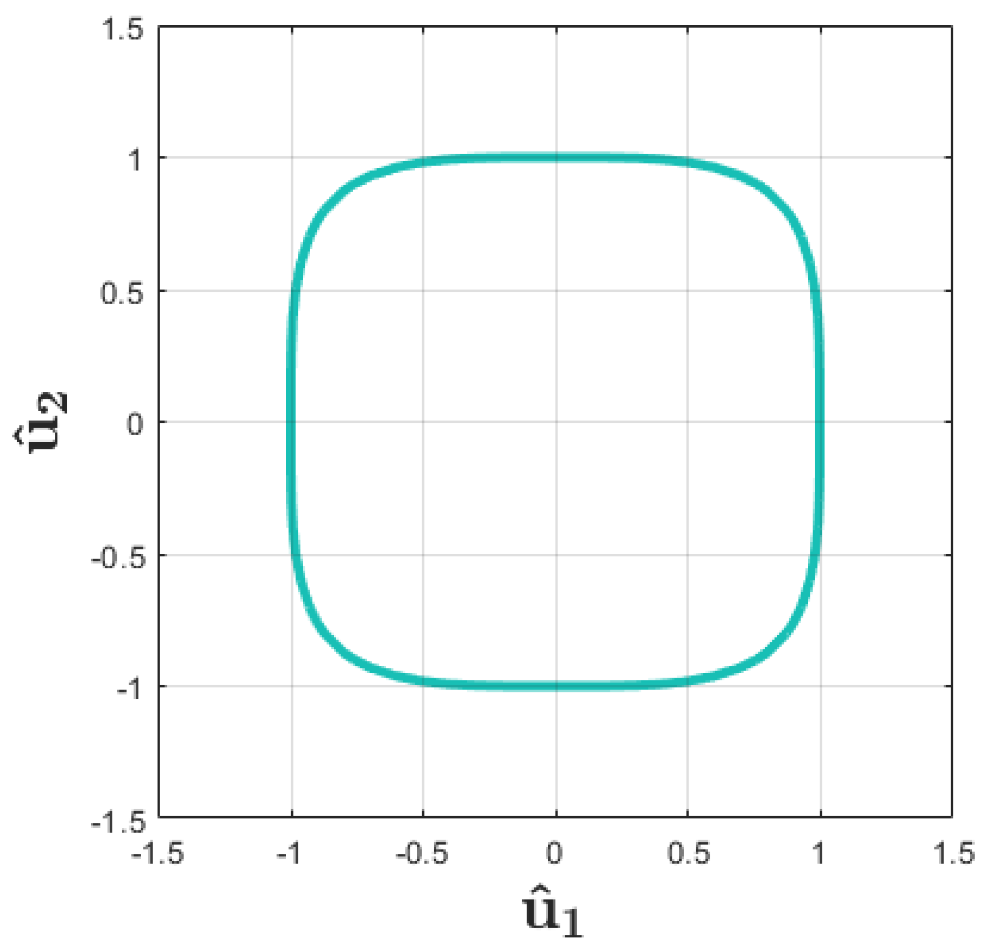
In Figure 4, the particular case of two-dimensional biquadratic surface $\mathbb{Q}\left(\widehat{\mathit{u}}\right)$ can be observed; from a practical point of view, this situation corresponds to afford the problem of estimating the maximum values of the AURV body accelerations $\dot{\mathit{\nu }}$ given the quasimaximum value of the thruster rotational speeds. For the sake of completeness, the term “quasimaximum” is used in this work to outline the fact the system inputs will never reach their maximum value at the same time, as shown in Figure 4.

Turning to a geometric interpretation of $\mathbb{Q}\left(\widehat{\mathit{u}}\right)$, the set of all propeller rotational speeds, at the input to the dynamic system defined in Equation (31), can be formulated as

$${\left({\widehat{\mathit{u}}}^2\right)}^T{\widehat{\mathit{u}}}^2=1$$

(33)

where ${\widehat{\mathit{u}}}^2$ is defined as

$${\widehat{\mathit{u}}}^2=J{\left(\mathit{q}\right)}^{†}(\dot{\mathit{\nu }}+{\dot{\mathit{\nu }}}_{\Gamma }({\mathit{\nu }}_r,\mathit{q},\mathit{\eta }))$$

(34)

which leads to

$${(\dot{\mathit{\nu }}+{\dot{\mathit{\nu }}}_{\Gamma }({\mathit{\nu }}_r,\mathit{q},\mathit{\eta }))}^T\left({\left(J{\left(\mathit{q}\right)}^{†}\right)}^{T}J{\left(\mathit{q}\right)}^{†}\right)(\dot{\mathit{\nu }}+{\dot{\mathit{\nu }}}_{\Gamma }({\mathit{\nu }}_r,\mathit{q},\mathit{\eta }))=1$$

(35)

where the operator ${(·)}^{†}$ refers to the Moore–Penrose pseudoinverse. The Equation (35) represents the dynamic maneuverability ellipsoid (DME) of the dynamic system described in Equation (31), defined as the set of the possible body-fixed accelerations $\dot{\mathit{\nu }}$ given the biquadratic surface $\mathbb{Q}\left(\widehat{\mathit{u}}\right)$ as input, and the acceleration ${\dot{\mathit{\nu }}}_{\Gamma }({\mathit{\nu }}_r,\mathit{q},\mathit{\eta })$ provided by the nonlinear forces. As a matter of fact, the nonlinear accelerations ${\dot{\mathit{\nu }}}_{\Gamma }({\mathit{\nu }}_r,\mathit{q},\mathit{\eta })$ result in a translation of the DME center, while it can be observed how the deformation (i.e., the length of the semiaxis) of the DME is related to the Jacobian $J\left(\mathit{q}\right)=M^{-1}\left(\mathit{q}\right)T\left(\mathit{q}\right)\mathbf{sgn}\left(\widehat{\mathit{u}}\right)$. In light of these considerations, the volume of the DME only depends on the chosen propulsion system, on the physical properties of the AURV, and on the thruster configuration on the actual configuration. A more exhaustive explanation can be provided by considering the singular value decomposition (SVD) of $J\left(\mathit{q}\right)$ [19],

$$\begin{array}{ccc}\hfill J& =& U\Sigma V^T=U\left[\begin{array}{cc}{diag}_{r\times r}\left({\sigma }_1,\dots ,{\sigma }_r\right)& 0_{\left(r\right)\times (m-r)}\\ 0_{(6-r)\times r}& 0_{(6-r)\times (m-r)}\end{array}\right]V^T\hfill \end{array}$$

(36)

$$\begin{array}{ccc}\hfill J^{+}& =& V{\Sigma }^{+}{U}^T=V\left[\begin{array}{cc}{diag}_{r\times r}\left(1/{\sigma }_1,\dots ,1/{\sigma }_r\right)& 0_{\left(r\right)\times (6-r)}\\ 0_{(n-r)\times r}& 0_{(m-r)\times (6-r)}\end{array}\right]U^T\hfill \end{array}$$

(37)

where $\Sigma \in R^{6\times m}$ contains the r nonzero singular values ${\sigma }_i$ of $J\left(\mathit{q}\right)$ in decreasing order, $U\in {\mathbb{R}}^{6\times 6}$ is an orthogonal matrix whose columns are the left singular vectors of $J\left(\mathit{q}\right)$ that form an orthonormal base of the output space, and $V\in {\mathbb{R}}^{m\times m}$ is an orthogonal matrix whose columns are the right singular vectors of $J\left(\mathit{q}\right)$ that form an orthonormal base of the input space. Furthermore, considering that

$$\begin{array}{ccc}\hfill {\Sigma }^{+}\in {\mathbb{R}}^{m\times 6}:{\Sigma }^{+}& =& \left[\begin{array}{cc}{diag}_{r\times r}\left(1/{\sigma }_1,\dots ,1/{\sigma }_r\right)& 0_{\left(r\right)\times (6-r)}\\ 0_{(n-r)\times r}& 0_{(m-r)\times (6-r)}\end{array}\right]\hfill \end{array}$$

(38)

$$\begin{array}{ccc}\hfill {\Sigma }^{+T}\in {\mathbb{R}}^{6\times m}:{\Sigma }^{+T}& =& \left[\begin{array}{cc}{diag}_{r\times r}\left(1/{\sigma }_1,\dots ,1/{\sigma }_r\right)⋮& 0_{\left(r\right)\times (m-r)}\\ 0_{(6-r)\times r}& 0_{(6-r)\times (m-r)}\end{array}\right]\hfill \end{array}$$

(39)

$$\begin{array}{ccc}\hfill \left({\Sigma }^{+T}{\Sigma }^{+}\right)& =& \left[\begin{array}{cc}error\left(1/{\sigma }_1^2,\dots ,1/{\sigma }_r^2\right)& 0_{\left(r\right)\times (6-r)}\\ 0_{(6-r)\times r}& 0_{(6-r)\times (6-r)}\end{array}\right]\in {\mathbb{R}}^{6\times 6},\hfill \end{array}$$

(40)

and inserting Equations (37), (36), and (40) in Equation (35), it results in the formulation of the DME expressed in the base of the left singular vectors of $\dot{\mathit{\nu }}+{\dot{\mathit{\nu }}}_{\Gamma }({\mathit{\nu }}_r,\mathit{q},\mathit{\eta })$, as follows

$$\begin{array}{ccc}\hfill {\mathit{w}}^T\left({\Sigma }^{+T}{\Sigma }^{+}\right)\mathit{w}& =& 1\hfill \end{array}$$

(41)

$$\begin{array}{ccc}\hfill \mathit{w}& =& U^T(\dot{\mathit{\nu }}+{\dot{\mathit{\nu }}}_{\Gamma }({\mathit{\nu }}_r,\mathit{q},\mathit{\eta })),\mathit{w}\in {\mathbb{R}}^6.\hfill \end{array}$$

(42)

Equation (41) describes the relationship among the singular values ${\sigma }_i$ of $J\left(\mathit{q}\right)$ and the DME. In greater detail, it can be observed that the singular values ${\sigma }_i$ represent the length of the DME semiaxis, expressed as in Equation (41), whereas their direction in the body-fixed frame can be obtained from the ith column of the matrix $\mathit{U}=[\cdots U_i\cdots ]$. Finally, from a practical consideration, the DME expressed in Equation (35) is studied in a decoupled manner from the linear ${\dot{\mathit{\nu }}}_1$ and angular ${\dot{\mathit{\nu }}}_2$ accelerations point of view. Thus, by defining

$$J\left(\mathit{q}\right)=\left[\begin{array}{c}{J}_1\left(\mathit{q}\right)\hfill \\ J_2\left(\mathit{q}\right)\hfill \end{array}\right],$$

(43)

the linear DME and the angular DME are evaluated, such as

$$\begin{array}{ccc}\hfill {({\dot{\mathit{\nu }}}_1+{\dot{\mathit{\nu }}}_{\Gamma 1}({\mathit{\nu }}_r,\mathit{q},\mathit{\eta }))}^T\left({\left(J_1^{†}\left(\mathit{q}\right)\right)}^T{J}_1^{†}\left(\mathit{q}\right)\right)({\dot{\mathit{\nu }}}_1+{\dot{\mathit{\nu }}}_{\Gamma 1}({\mathit{\nu }}_r,\mathit{q},\mathit{\eta }))& =& 1\hfill \end{array}$$

(44)

$$\begin{array}{ccc}\hfill {({\dot{\mathit{\nu }}}_2+{\dot{\mathit{\nu }}}_{\Gamma 2}({\mathit{\nu }}_r,\mathit{q},\mathit{\eta }))}^T\left({\left(J_2^{†}\left(\mathit{q}\right)\right)}^T{J}_2^{†}\left(\mathit{q}\right)\right)({\dot{\mathit{\nu }}}_2+{\dot{\mathit{\nu }}}_{\Gamma 2}({\mathit{\nu }}_r,\mathit{q},\mathit{\eta }))& =& 1.\hfill \end{array}$$

(45)

For the sake of completeness, the well-known formulations of Equations (41) and (37) can be extended for both the linear and angular ellipsoids defined in Equations (44) and (45).

6. Metrics and Indices

As described above, the linear and angular DMEs provides a qualitative geometric evaluation of the maneuverability of an AURV configuration; conversely, quantitative indices will be outlined in this Section. More specifically, Yoshikawa’s manipulability index [10,11] is defined as

$$W_1\left(\mathit{q}\right)=\sqrt{J\left(\mathit{q}\right)J{\left(\mathit{q}\right)}^T}=\prod _{i=1}^6{\sigma }_i$$

(46)

which is proportional to the volume of the DME. Therefore, it can be used to numerically evaluate the overall maneuverability of the system by exploiting the following concept: a larger volume reflects a better performance. The Equation (46) does not consider if the vehicle is near a “singularity”, i.e., a situation where the vehicle cannot move in a direction ${\mathit{U}}_i$ associated to a singular value ${\sigma }_i=0$. Thus, a second manipulability index is often associated with the inverse of condition number $k_2\left(J\left(\mathit{q}\right)\right)$ of the Jacobian matrix $J\left(\mathit{q}\right)$ as

$$\begin{array}{ccc}\hfill W_2\left(\mathit{q}\right)=\frac{1}{k_2\left(J\left(\mathit{q}\right)\right)}& =& \frac{{\sigma }_{min}}{{\sigma }_{max}}\hfill \end{array}$$

(47)

$$\begin{array}{ccc}\hfill k_2\left(J\left(\mathit{q}\right)\right)={\parallel J\left(\mathit{q}\right)\parallel }_2{∥J^{†}\left(\mathit{q}\right)∥}_2& =& \frac{{\sigma }_{max}}{{\sigma }_{min}}.\hfill \end{array}$$

(48)

The aforementioned index is considerably appealing since immediately provides useful information: firstly, it can be observed that this index represents the ellipsoid eccentricity; then, if the vehicle is not omnidirectional (i.e., cannot move in every degree of freedom), the index defined in Equation (47) holds to a zero value. Finally, the authors propose a third index as an absolute value of the AURV maneuverability in the three different directions of the body-fixed frame. As described in Section 5, the problem of estimating the maximum values of the AURV body accelerations $\dot{\mathit{\nu }}$ given the quasimaximum value of the thruster rotational speeds have been addressed in this work. From a more practical as well as physical perspective, it can be seen as a way to measure the difference between the maximum admissible linear ${\dot{\mathit{\nu }}}_1$ and angular ${\dot{\mathit{\nu }}}_2$ accelerations along each axis of the body-fixed reference frame. As a result, for the linear and angular DMEs, these indices can be defined as

$${}^j{W}_3\left(\mathit{q}\right)=\underset{i}{max}\left|{({\sigma }_i{\mathit{U}}_i+{\dot{\mathit{\nu }}}_{\Gamma }({\mathit{\nu }}_r,\mathit{q},\mathit{\eta }))}^T{\mathit{l}}_j\right|,i,j=1,2,3,$$

(49)

where ${\mathit{l}}_j\in {\mathbb{R}}^3$ is the unit vector identifying the jth direction of the AURV linear/angular motion.

7. Simulations and Results

The maneuverability simulation performed for both the extreme UNIFI DIEF configurations are presented in this Section. Within the context of this work, the following notation is employed: a generic property $A\left({\mathit{q}}_1\right)$ belongs to the “survey” AURV configuration, while $A\left({\mathit{q}}_2\right)$ relates to a feature of the “hovering” one. Furthermore, the results hereafter presented have been obtained by means of MATLAB-coded dynamic simulations. In particular, along with the assumptions proposed in Section 3, the following settings have been used:

• the AURV position ${\mathit{\eta }}_1$ is the same in both the two configurations, and the vehicle orientation ${\mathit{\eta }}_2$ will be expressed with respect to the NED frame. Additionally, it is assumed that the vehicle is in resting position (i.e., $\mathit{\nu }={\mathbf{0}}_{6\times 1}$) affected by the marine currents. Although this hypothesis may seem restrictive, it was decided, within this preliminary study, to consider the scenario in which the AURV, in both the configurations, is stationary; realistic cases of motion will be investigated in the future. The kinematic parameters are summarized in

  Table 1. Main kinematic parameters.

  NED position (m):	${\mathit{\eta }}_1={[0.0,0.0,1.0]}^{\mathit{T}}$
  NED orientation (RPY) $\left[rad\right]$:	${\mathit{\eta }}_2={[0.0,0.0,0.0]}^T$
  Linear relative body-fixed velocity (m/s):	${\mathit{\nu }}_{1r}={[-0.4,0.0,0.0]}^T$
  Angular relative body-fixed velocity (rad/s):	${\mathit{\nu }}_{2r}={[0.0,0.0,0.0]}^T$

  :
• The dynamic terms in Equation (4) have been evaluated by exploiting several preliminary hydrodynamic simulations. More accurate identification strategies will be further analyzed in the future in order to provide an accurate estimate of the AURV dynamic parameters. Therefore, the dynamic features of survey ${\mathit{q}}_1$ and hovering ${\mathit{q}}_2$ configurations are respectively listed in

  Table 2. UNIFI DIEF AURV dynamic parameters.

  Mass matrix:   $M\left({\mathit{q}}_1\right)=\left[\begin{array}{cccccc}\hfill 250.0& \hfill 0.0& \hfill 0.0& \hfill 0.0& \hfill 0.0& \hfill 0.0\\ \hfill 0.0& \hfill 250.0& \hfill 0.0& \hfill 0.0& \hfill 0.0& \hfill 0.0\\ \hfill 0.0& \hfill 0.0& \hfill 250.0& \hfill 0.0& \hfill 0.0& \hfill 0.0\\ \hfill 0.0& \hfill 0.0& \hfill 0.0& \hfill 10.7& \hfill 0.0& \hfill 0.0\\ \hfill 0.0& \hfill 0.0& \hfill 0.0& \hfill 0.0& \hfill 58.2& \hfill 0.0\\ \hfill 0.0& \hfill 0.0& \hfill 0.0& \hfill 0.0& \hfill 0.0& \hfill 65.3\end{array}\right]$

  Coriolis matrix:    $C({\mathit{\nu }}_r,{\mathit{q}}_1)=\left[\begin{array}{cccccc}\hfill 0.0& \hfill 0.0& \hfill 0.0& \hfill 0.0& \hfill 0.0& \hfill 0.0\\ \hfill 0.0& \hfill 0.0& \hfill 0.0& \hfill 0.0& \hfill 0.0& \hfill 100.0\\ \hfill 0.0& \hfill 0.0& \hfill 0.0& \hfill 0.0& \hfill -100.0& \hfill 0.0\\ \hfill 0.0& \hfill 0.0& \hfill 0.0& \hfill 0.0& \hfill 0.0& \hfill 0.0\\ \hfill 0.0& \hfill 0.0& \hfill 100.0& \hfill 0.0& \hfill 0.0& \hfill 0.0\\ \hfill 0.0& \hfill -100.0& \hfill 0.0& \hfill 0.0& \hfill 0.0& \hfill 0.0\end{array}\right]$

  Damping matrix:    $D({\mathit{\nu }}_r,{\mathit{q}}_1)=\left[\begin{array}{cccccc}\hfill -21.5& 0.0& 0.0& 0.0& 0.0& 0.0\\ \hfill 0.0& 0.0& 0.0& 0.0& 0.0& 0.0\\ \hfill 0.0& 0.0& 0.0& 0.0& 0.0& 0.0\\ \hfill 0.0& 0.0& 0.0& 0.0& 0.0& 0.0\\ \hfill 0.0& 0.0& 0.0& 0.0& 0.0& 0.0\\ \hfill 0.0& 0.0& 0.0& 0.0& 0.0& 0.0\end{array}\right]$

  Gravity and Buoyancy vector:    $\mathbf{g}\left(\mathit{\eta }\right)={[0.0,0.0,-12.2,0.0,0.0,0.0]}^T$

  Mass matrix:   $M\left({\mathit{q}}_2\right)=\left[\begin{array}{cccccc}\hfill 250.0& \hfill 0.0& \hfill 0.0& \hfill 0.0& \hfill 0.0& \hfill 0.0\\ \hfill 0.0& \hfill 250.0& \hfill 0.0& \hfill 0.0& \hfill 0.0& \hfill 0.0\\ \hfill 0.0& \hfill 0.0& \hfill 250.0& \hfill 0.0& \hfill 0.0& \hfill 0.0\\ \hfill 0.0& \hfill 0.0& \hfill 0.0& \hfill 49.2& \hfill 0.0& \hfill 0.0\\ \hfill 0.0& \hfill 0.0& \hfill 0.0& \hfill 0.0& \hfill 31.6& \hfill 0.0\\ \hfill 0.0& \hfill 0.0& \hfill 0.0& \hfill 0.0& \hfill 0.0& \hfill 77.2\end{array}\right]$

  Coriolis matrix:    $C({\mathit{\nu }}_r,{\mathit{q}}_2)=\left[\begin{array}{cccccc}\hfill 0.0& \hfill 0.0& \hfill 0.0& \hfill 0.0& \hfill 0.0& \hfill 0.0\\ \hfill 0.0& \hfill 0.0& \hfill 0.0& \hfill 0.0& \hfill 0.0& \hfill 100.0\\ \hfill 0.0& \hfill 0.0& \hfill 0.0& \hfill 0.0& \hfill -100.0& \hfill 0.0\\ \hfill 0.0& \hfill 0.0& \hfill 0.0& \hfill 0.0& \hfill 0.0& \hfill 0.0\\ \hfill 0.0& \hfill 0.0& \hfill 100.0& \hfill 0.0& \hfill 0.0& \hfill 0.0\\ \hfill 0.0& \hfill -100.0& \hfill 0.0& \hfill 0.0& \hfill 0.0& \hfill 0.0\end{array}\right]$

  Damping matrix:    $D({\mathit{\nu }}_r,{\mathit{q}}_2)=\left[\begin{array}{cccccc}\hfill -41.2& 0.0& 0.0& 0.0& 0.0& 0.0\\ \hfill 0.0& 0.0& 0.0& 0.0& 0.0& 0.0\\ \hfill 0.0& 0.0& 0.0& 0.0& 0.0& 0.0\\ \hfill 0.0& 0.0& 0.0& 0.0& 0.0& 0.0\\ \hfill 0.0& 0.0& 0.0& 0.0& 0.0& 0.0\\ \hfill 0.0& 0.0& 0.0& 0.0& 0.0& 0.0\end{array}\right]$

  Gravity and buoyancy vector:    $\mathbf{g}\left(\mathit{\eta }\right)={[0.0,0.0,-12.2,0.0,0.0,0.0]}^T$

  .
• The two different thrust allocation matrices $B\left(\mathit{q}\right)$ have been evaluated by using the body-fixed position ${\mathit{r}}_i$ and longitudinal direction ${\mathit{n}}_i$ of the ith thruster in both configurations, estimated in the design stage of the AURV. As a result,

  Table 3. UNIFI DIEF AURV thrust configuration parameters.

  Thruster positions $\left({\mathit{q}}_1\right)\left[m\right]$:    $\begin{array}{c}{\mathit{r}}_{\mathbf{1}}=[0.7,-0.4,0.0]\\ {\mathit{r}}_{\mathbf{2}}=[0.7,0.4,0.0]\\ {\mathit{r}}_{\mathbf{3}}=[-0.7,-0.4,0.0]\\ {\mathit{r}}_{\mathbf{4}}=[-0.7,0.4,0.0]\\ {\mathit{r}}_{\mathbf{5}}=[0.0,-0.3,0.0]\\ {\mathit{r}}_{\mathbf{6}}=[0.0,0.3,0.0]\\ {\mathit{r}}_{\mathbf{7}}=[0.8,0.0,0.0]\\ {\mathit{r}}_{\mathbf{8}}=[-0.8,0.0,0.0]\end{array}$

  Thruster longitudinal axis $\left({\mathit{q}}_1\right)\left[rad\right]$:    $\begin{array}{c}{\theta }_1=\frac{\pi }{2},{\phi }_1=0.0\\ {\theta }_2=\frac{\pi }{2},{\phi }_2=0.0\\ {\theta }_3=\frac{\pi }{2},{\phi }_3=0.0\\ {\theta }_4=\frac{\pi }{2},{\phi }_4=0.0\\ {\theta }_5=0.0,{\phi }_5=0.0\\ {\theta }_6=0.0,{\phi }_6=0.0\\ {\theta }_7=0.0,{\phi }_7=0.0\\ {\theta }_8=0.0,{\phi }_8=0.0\end{array}$

  TAM:    $B\left({\mathit{q}}_1\right)=\left[\begin{array}{cccccccc}\hfill 1.0& \hfill 1.0& \hfill 1.0& \hfill 1.0& \hfill 0.0& \hfill 0.0& \hfill 0.0& \hfill 0.0\\ \hfill 0.0& \hfill 0.0& \hfill 0.0& \hfill 0.0& \hfill 0.0& \hfill 0.0& \hfill 0.0& \hfill 0.0\\ \hfill 0.0& \hfill 0.0& \hfill 0.0& \hfill 0.0& \hfill 1.0& \hfill 1.0& \hfill 1.0& \hfill 1.0\\ \hfill 0.0& \hfill 0.0& \hfill 0.0& \hfill 0.0& \hfill -0.3& \hfill 0.3& \hfill 0.0& \hfill 0.0\\ \hfill 0.0& \hfill 0.0& \hfill 0.0& \hfill 0.0& \hfill 0.0& \hfill 0.0& \hfill -0.8& \hfill 0.8\\ \hfill 0.4& \hfill -0.4& \hfill 0.4& \hfill -0.4& \hfill 0.0& \hfill 0.0& \hfill 0.0& \hfill 0.0\end{array}\right]$

  Thruster positions $\left({\mathit{q}}_2\right)\left[m\right]$:    $\begin{array}{c}{\mathit{r}}_{\mathbf{1}}=[0.6,-0.5,0.0]\\ {\mathit{r}}_{\mathbf{2}}=[0.6,0.5,0.0]\\ {\mathit{r}}_{\mathbf{3}}=[-0.6,-0.5,0.0]\\ {\mathit{r}}_{\mathbf{4}}=[-0.6,0.5,0.0]\\ {\mathit{r}}_{\mathbf{5}}=[0.0,-1.0,0.0]\\ {\mathit{r}}_{\mathbf{6}}=[0.0,1.0,0.0]\\ {\mathit{r}}_{\mathbf{7}}=[0.6,-0.0,0.0]\\ {\mathit{r}}_{\mathbf{8}}=[-0.6,-0.0,0.0]\end{array}$

  Thruster longitudinal axis $\left({\mathit{q}}_2\right)\left[rad\right]$:    $\begin{array}{c}{\theta }_1=\frac{\pi }{2},{\phi }_1=\frac{\pi }{4}\\ {\theta }_2=\frac{\pi }{2},{\phi }_2=-\frac{\pi }{4}\\ {\theta }_3=\frac{\pi }{2},{\phi }_3=-\frac{\pi }{4}\\ {\theta }_4=\frac{\pi }{2},{\phi }_4=\frac{\pi }{4}\\ {\theta }_5=0.0,{\phi }_5=0.0\\ {\theta }_6=0.0,{\phi }_6=0.0\\ {\theta }_7=0.0,{\phi }_7=0.0\\ {\theta }_8=0.0,{\phi }_8=0.0\end{array}$

  TAM:    $B\left({\mathit{q}}_2\right)=\left[\begin{array}{cccccccc}\hfill 0.7& \hfill 0.7& \hfill 0.7& \hfill 0.7& \hfill 0.0& \hfill 0.0& \hfill 0.0& \hfill 0.0\\ \hfill 0.7& \hfill -0.7& \hfill -0.7& \hfill 0.7& \hfill 0.0& \hfill 0.0& \hfill 0.0& \hfill 0.0\\ \hfill 0.0& \hfill 0.0& \hfill 0.0& \hfill 0.0& \hfill 1.0& \hfill 1.0& \hfill 1.0& \hfill 1.0\\ \hfill 0.0& \hfill 0.0& \hfill 0.0& \hfill 0.0& \hfill -0.9& \hfill -0.9& \hfill 0.0& \hfill 0.0\\ \hfill 0.0& \hfill 0.0& \hfill 0.0& \hfill 0.0& \hfill 0.0& \hfill 0.0& \hfill -0.6& \hfill 0.6\\ \hfill 0.8& \hfill -0.8& \hfill 0.8& \hfill -0.8& \hfill 0.0& \hfill 0.0& \hfill 0.0& \hfill 0.0\end{array}\right]$

  shows the thruster configurations parameters, where the ith thruster longitudinal axis have been expressed in the terms of the inclination ${\theta }_i$ and azimuth ${\phi }_i$ angle in spherical coordinates.
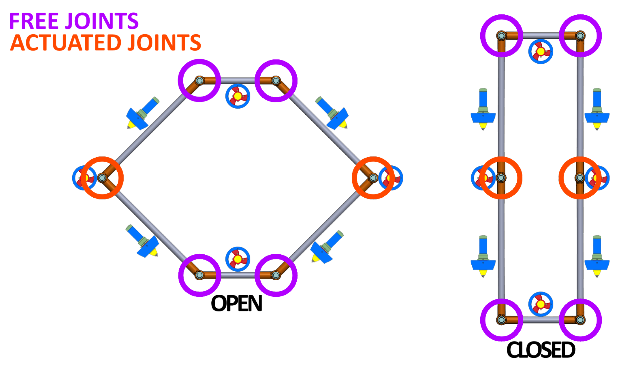
  It can be straightforwardly observed, as already described in the Section 2, how the first four thrusters are necessary for the linear motion of the vehicle along the horizontal plane, whereas the last four provide displacement along the vertical direction of the body-fixed frame. In particular, Table 3, shows how the first four thrusters are all aligned along the surge axis in the survey configuration, with the aim of improving the longitudinal navigation, whilst, at the same time, the AURV cannot move in the sway direction.
• With regard to the propulsion system parameters,

  Table 4. T200 BlueRobotics Thruster model parameters.

  Propeller pitch: $[m/rev]$	$0.09$
  Forward bollard coefficient: $\left[N{s}^2\right]$	$0.0128$
  Backward bollard coefficient: $\left[N{s}^2\right]$	$-0.008753$
  Forward dead-zone boundary limit: $\left[Hz\right]$	$4.8833+0.5866(\mathcal{V}-14)$
  Backward dead-zone boundary limit: $\left[Hz\right]$	$-4.8167-0.5974(\mathcal{V}-14)$
  Maximum speed: $\left[rpm\right]$	2400

  outlines the estimated values for the BlueRobotics T200 propeller [20], the motor selected to be equipped in the UNIFI DIEF AURV; it is worth noticing how these values have been evaluated by exploiting the methodology described from the authors in [21].

As highlighted in Section 4, in this work, a preliminary assumption has been done by neglecting the dead-zone boundary values and the term depending upon the motor advance speed. Indeed, we approximate the relationship among the motor rotational speed and the longitudinal thrust with the forward bollard coefficient defined in Table 4.

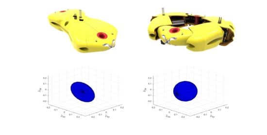
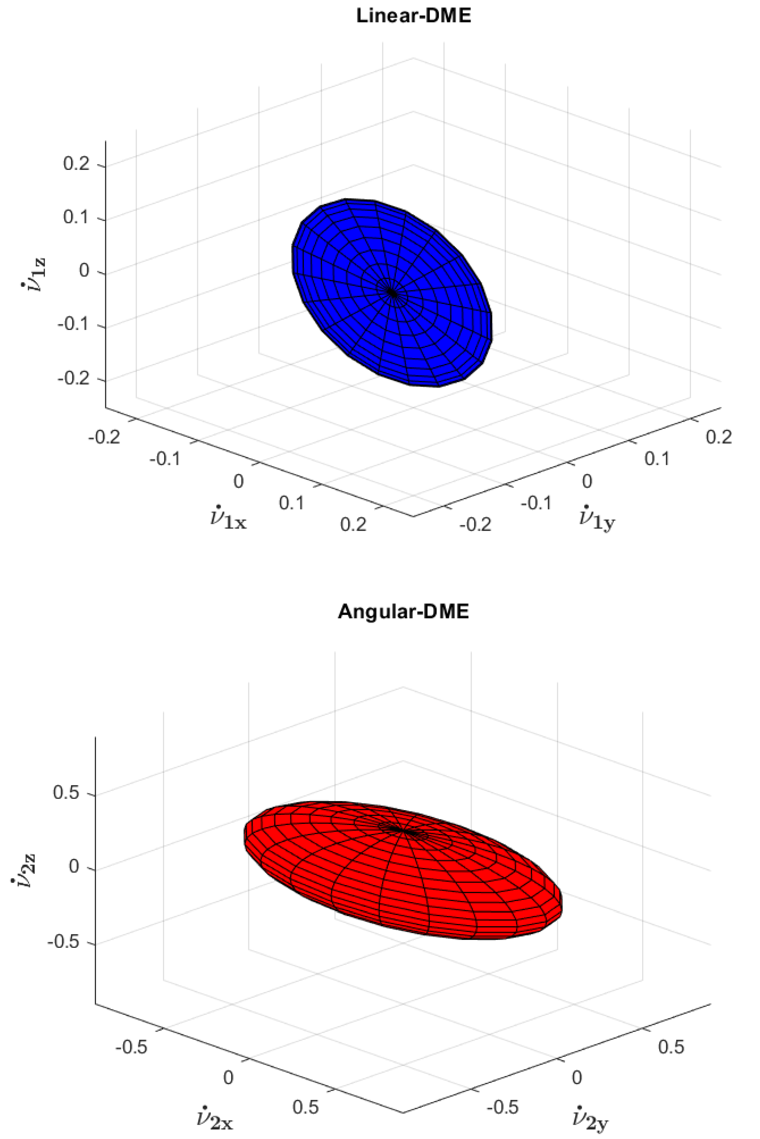
The above-illustrated parameters have been employed in order to obtain the linear DME and angular DME, described in Equations (44) and (45), and the maneuverability indices defined in Equations (46)–(49) in Section 6, for both the configurations of the UNIFI DIEF AURV. Figure 5, illustrates the angular and linear ellipsoids for the survey shape of the vehicle. In particular, it is worth noticing how the linear DME turns to a circle, since the singular value related to the sway direction is equal to zero, as observed in the

Table 5. Quantitative maneuverability indices for the UNIFI DIEF AURV.

Survey Configuration
Linear DME	Angular DME
${\sigma }_1\left({\mathit{q}}_1\right)=0.164,{\mathit{U}}_1={[1,0,0]}^T$	${\sigma }_1\left({\mathit{q}}_1\right)=0.839,{\mathit{U}}_1={[1,0,0]}^T$
${\sigma }_2\left({\mathit{q}}_1\right)=0.164,{\mathit{U}}_2={[0,0,1]}^T$	${\sigma }_2\left({\mathit{q}}_1\right)=0.420,{\mathit{U}}_2={[0,1,0]}^T$
${\sigma }_3\left({\mathit{q}}_1\right)=0.0,{\mathit{U}}_3={[0,1,0]}^T$	${\sigma }_3\left({\mathit{q}}_1\right)=0.267,{\mathit{U}}_3={[0,0,1]}^T$
$W_1\left({\mathit{q}}_1\right)=0.0$	$W_1\left({\mathit{q}}_1\right)=0.094$
$W_2\left({\mathit{q}}_1\right)=0.0$	$W_2\left({\mathit{q}}_1\right)=0.318$
${}^x{W}_3\left({\mathit{q}}_1\right)=0.128$	${}^x{W}_3\left({\mathit{q}}_1\right)=0.838$
${}^z{W}_3\left({\mathit{q}}_1\right)=0.115$	${}^y{W}_3\left({\mathit{q}}_1\right)=0.420$
${}^y{W}_3\left({\mathit{q}}_1\right)=0.0$	${}^z{W}_3\left({\mathit{q}}_1\right)=0.266$
Hovering Configuration
Linear DME	Angular DME
${\sigma }_1\left({\mathit{q}}_1\right)=0.164,{\mathit{U}}_1={[0,0,1]}^T$	${\sigma }_1\left({\mathit{q}}_1\right)=0.587,{\mathit{U}}_1={[0,1,0]}^T$
${\sigma }_2\left({\mathit{q}}_1\right)=0.116,{\mathit{U}}_2={[1,0,0]}^T$	${\sigma }_2\left({\mathit{q}}_1\right)=0.565,{\mathit{U}}_2={[1,0,0]}^T$
${\sigma }_3\left({\mathit{q}}_1\right)=0.116,{\mathit{U}}_3={[0,1,0]}^T$	${\sigma }_3\left({\mathit{q}}_1\right)=0.437,{\mathit{U}}_3={[0,0,1]}^T$
$W_1\left({\mathit{q}}_2\right)=0.022$	$W_1\left({\mathit{q}}_2\right)=0.145$
$W_2\left({\mathit{q}}_2\right)=0.707$	$W_2\left({\mathit{q}}_2\right)=0.745$
${}^x{W}_3\left({\mathit{q}}_2\right)=0.050$	${}^x{W}_3\left({\mathit{q}}_2\right)=0.565$
${}^y{W}_3\left({\mathit{q}}_2\right)=0.067$	${}^y{W}_3\left({\mathit{q}}_2\right)=0.587$
${}^z{W}_3\left({\mathit{q}}_2\right)=0.115$	${}^z{W}_3\left({\mathit{q}}_2\right)=0.437$

; thus, Yoshikawa’s index $W_1\left({\mathit{q}}_1\right)$ and $W_2\left({\mathit{q}}_1\right)$ are also a zero value. 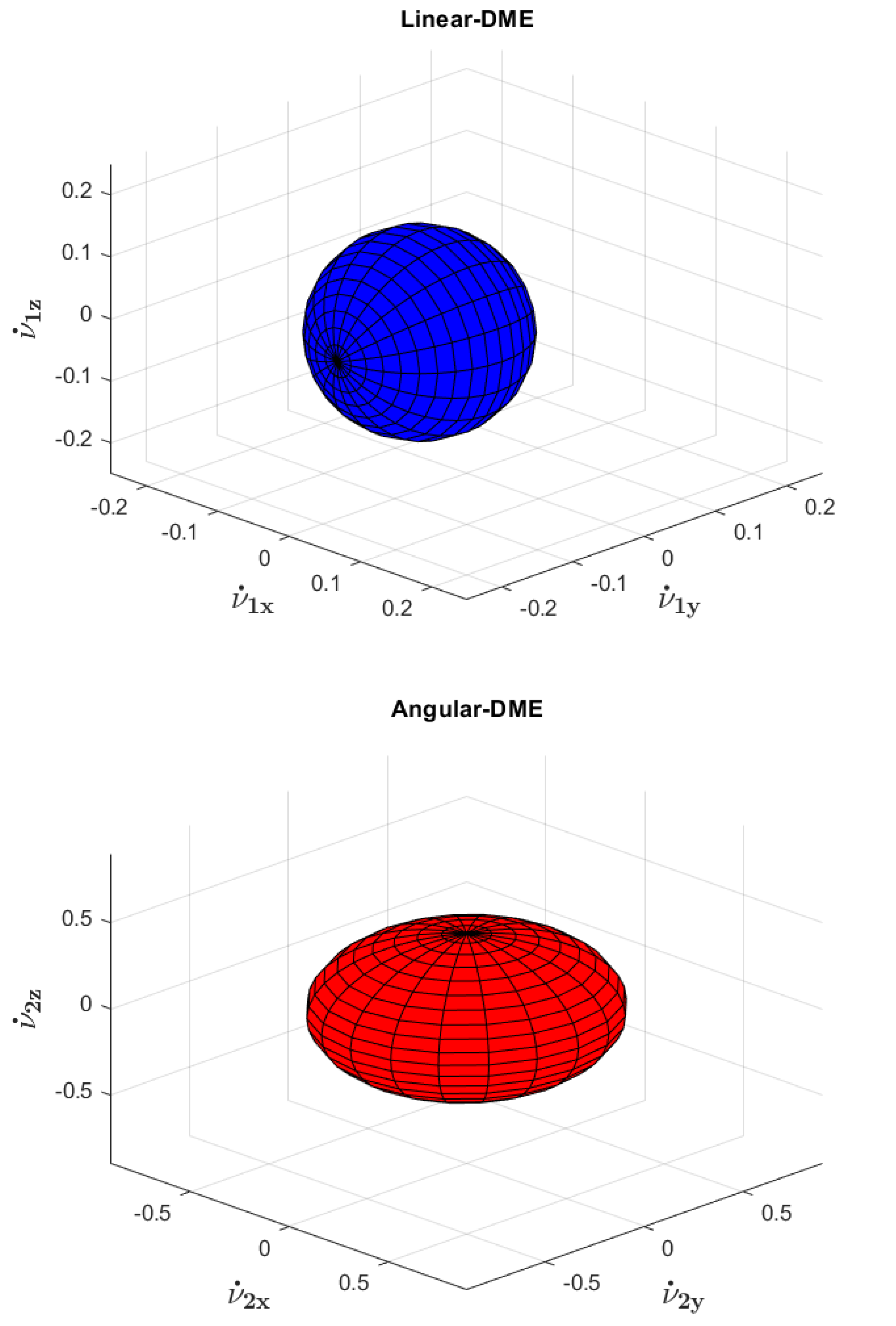If these results define the survey configuration as a singular one (i.e., the motion on the sway axis of the body-fixed frame is not taken into account), it should be considered as the index ${}^x{W}_3\left({\mathit{q}}_1\right)$, defined as the maximum values of the AURV body accelerations $\dot{\mathit{\nu }}$, along the surge x direction, given the quasimaximum value of the thruster rotational speeds as input, is much larger than the same index for the hovering configuration. Conversely, the hovering configuration has the property of a omnidirectional motion in all the six degrees of freedom, as shown in Figure 6, and, as a consequence, Yoshikawa’s index $W_1\left({\mathit{q}}_2\right)$ is different from zero. Additionally, it is interesting to notice that the index $W_2\left({\mathit{q}}_2\right)$ is closer to the unit value in both linear DME and angular DME, which implies that the hovering configuration is accurately controllable in every direction of space and can find a realistic application in complex tasks, as, for instance, working on an offshore structure or recovering samples from a shipwreck. 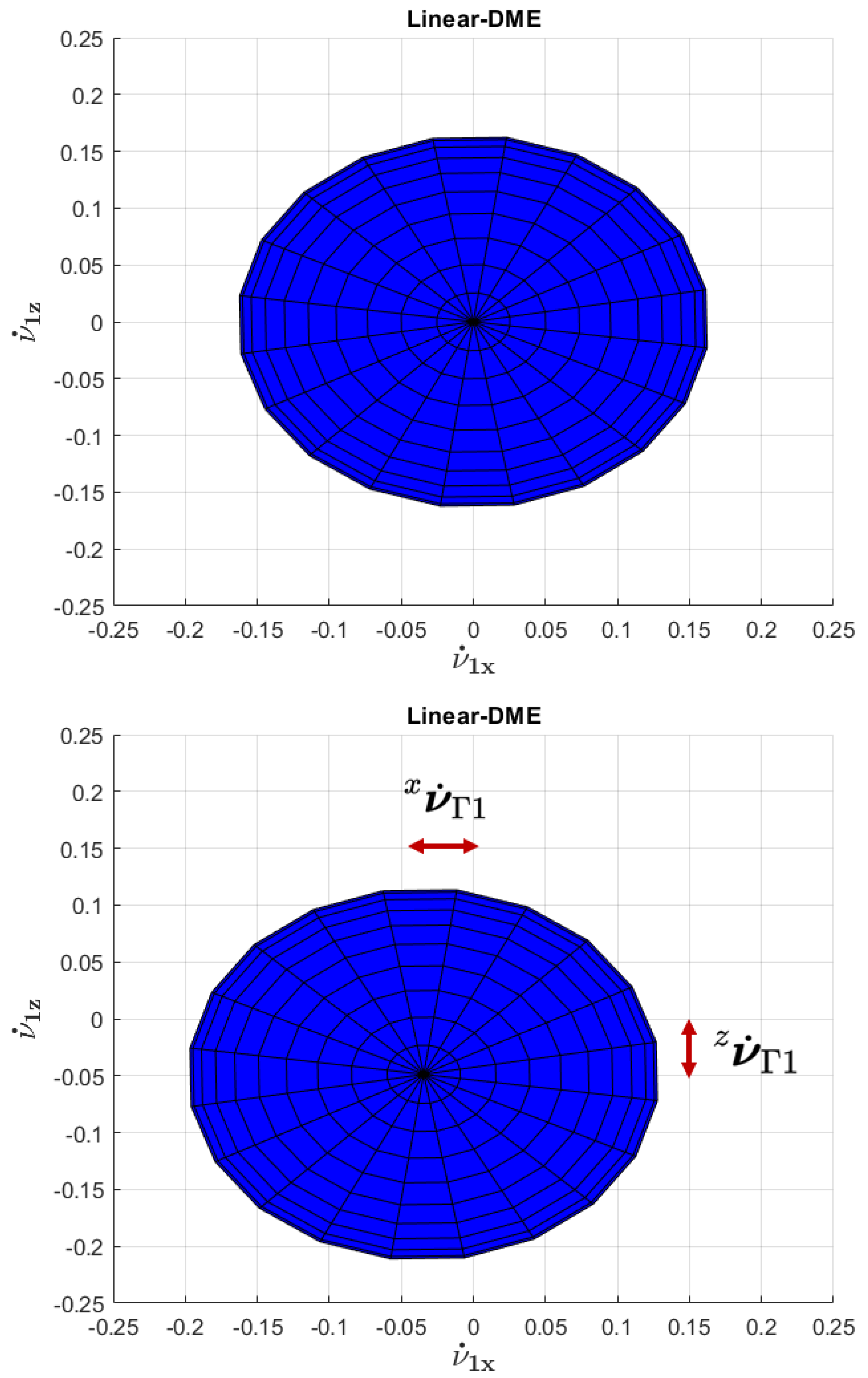Furthermore, Figure 7 illustrates the linear DME for the survey configuration in two different situations: firstly, when the ellipsoid is calculated considering to be in the absence of accelerations due to nonlinear terms (i.e., ${\dot{\mathit{\nu }}}_{\Gamma }({\mathit{\nu }}_r,\mathit{q},\mathit{\eta })={\mathbf{0}}_{6\times 1}$), then with the assumptions explained at the beginning of this Section. As proposed in Section 5, the nonlinear accelerations ${\dot{\mathit{\nu }}}_{\Gamma }({\mathit{\nu }}_r,\mathit{q},\mathit{\eta })$ result in a translation of the linear DME center, while the shape of the linear DME is not affected, since it is only related to the singular values $\sigma \left(\mathit{q}\right)$. These considerations can also be applied in the case of the angular DME indeed. In conclusion, this section showed the results of the innovative dynamic maneuverability analysis on the UNIFI DIEF AURV obtained by means of dynamic simulations. From a qualitative point of view, linear and angular DMEs have been estimated for both the extreme configurations of the vehicle. As a first observation, it can be noted that such strategy allows immediately to distinguish if a vehicle is omnidirectional or if it is singular along a direction of motion. Additionally, several indices have been supplied as quantitative measurements of the AURV maneuverability. More specifically, the index proposed by the authors in Equation (49) represents the maximum value of the AURV body accelerations given the quasi-maximum value of the thruster rotational speeds. Therefore, this index can be used as a relevant absolute value of maneuverability for the different AURV configurations.

8. Conclusions

This work collects the results of the preliminary research activity on the dynamic maneuverability analysis (DMA) application on the innovative AURV designed by the Department of Industrial Engineering of the University of Florence [8,9]. As a matter of fact, autonomous underwater reconfigurable vehicles [3] do arise as a promising tool for incorporating several reconfigurable modules and accomplishing several complex tasks as intervention, maintenance, and repair (IMR) operations. The activity focused on the study of the maneuverability methodology for underwater vehicles, by starting from the analysis of state-of-the-art solutions in the field of robotics arm [10], and leading to the specific case-study of the UNIFI DIEF AURV. While the concept of maneuverability has already been studied in underwater robotics, as, for instance, for the thruster configuration optimization [12,13], we introduce a novel analysis which relates the vehicle body-fixed accelerations with the rotational speed of each thruster, taking into account also the AURV dynamic model for the several configurations, and the propulsion system assumed in the designing phase. It is worth noticing that, despite the specific application of this work, the proposed methodology can be applied to any unmanned underwater vehicle (UUV), if its dynamic and propulsion system parameters are correctly identified. In this context, the application of artificial intelligence (AI) algorithms has been arisen as innovative solutions for the identification of the UUV dynamic parameters, as suggested in [22]. As a result, further investigations and comparisons will be performed among the UNIFI DIEF AURV and other AUVs. Moreover, [14] inspires the possibility for further studies on multibody modeling for reconfigurable vehicles. The last, but not least, key topic which is worth being explored in the future is the introduction of all the nonlinear properties which have not been considered in the AURV dynamic model, as the estimate of the added mass terms as well as the dead-zone boundary values of the thrusters. All these open problems and research areas, whose resolution and deepening constitute a natural continuation of the cutting-edge research activity carried out thus far, will be subjected to further investigations in the near future.