Possibility of Bridge Inspection through Drive-By Vehicles

Abstract

Based on virtual simulations of vehicle–bridge interactions, the possibility of detecting stiffness reduction damages in bridges through vehicle responses was tested in two dimensional (2D) and three dimensional (3D) settings. Short-Time Fourier Transformation (STFT) was used to process vehicles’ acceleration data obtained through the 2D and 3D virtual simulations. The energy band variation of the vehicle acceleration time history was found strongly related to damage parameters. More importantly, the vehicle’s initial entering conditions are critical in obtaining correct vehicle responses through the vehicle bridge interaction models. The offset distance needed before executing the vehicle–bridge interaction (VBI) modeling was obtained through different road profile roughness levels. Through the above breakthroughs in VBI modeling, the presented study provides a new and integrated method for drive-by bridge inspection.

1. Background and Literature Review

With the massive amount of infrastructure built in US, the timely assessment of these infrastructures becomes critical to the public’s safety. Due to the high cost and time-consuming direct condition assessment methods, such as closing traffic for sensor installation and monitoring, indirect bridge monitoring has become a promising method to manage transportation infrastructure conditions.

The idea of indirect bridge assessment that uses a passing vehicle to detect dynamic bridge properties was initiated by Yang et al. in 2004 [1]. They built a numerical model of a bridge vehicle system and studied the possibility of extracting bridge frequencies from vehicles’ responses. Yang and Lin [2] further proposed a finite element model and verified the accuracy of the concept. The results clearly showed four frequencies in the acceleration spectrum: vehicle frequency, driving frequency, and two shifted bridge frequencies. However, the theoretical model is still a little far from applicable in practice because the model does not consider vehicle damping and multi-span effects of the bridge. In another Yang and Lin research [3], they studied more about the relationship of vehicle–bridge systems. In contrast to the previous model, the response of the bridge concentrates on its first vibration mode. The reason is that the vehicle, which acts as a moving force, cannot transfer much energy to trigger higher modes of a heavier bridge. Through comparison of the displacement, velocity, and acceleration responses of the bridge under five different vehicle speeds, it was found that the acceleration response is more sensitive on extracting bridge frequencies. Another tested parameter is the damping of the vehicle. It was found that the damping will decrease the amplitude of the acceleration spectrum, which may cause difficulty in identifying bridge frequencies. Yang and Chang further conducted a parametric study on this indirect method [4]. In this work, a more complicated response function was derived to describe the vehicle–bridge system and concluded that the initial vehicle/bridge acceleration amplitude ratio is important in identifying the bridge frequency. The smaller the ratio, the greater the probability of successfully identifying the bridge frequencies is.

Yang et al. also had another study to build the mode shape from a passing vehicle [5]. In this study, the bridge response’s instantaneous amplitude history can be regarded as a mode shape. However, the bridge’s vibration amplitude is always captured in absolute value, and the sign of the mode values needs to be decided first. González performed a simulation of extracting bridge frequency using vehicles under different conditions [6]. In this study, a 3D vehicle and bridge finite element models were built using MSc/NASTRAN software. In the simulation, the first natural frequency of the bridge is not found in various vehicle speeds. González conducted a further study on extracting bridge frequency and damping [7]. The model adopted was a 2D half vehicle and bridge model simulated in MATLAB. Three different length bridges with five different damping conditions were simulated. By increasing the bridge length, the power spectrum (higher amplitude) will shift to higher frequencies. If damping and the road roughness were considered, the acceleration spectra itself sometimes could not show the bridge frequency due to energy dissipation caused by damping and road roughness. However, the power spectrum’s sensitivity at all frequencies with respect to damping level changes can still show the bridge frequency.

Zhang and his team performed a damage detection study based on the bridge mode shapes [8]. In their study, the Short-Time Fourier Transformation (STFT) acceleration spectrum’s amplitude is approximately proportional to the mode shape square (MOSS). Furthermore, the mode shape square can show obvious differences between damage and undamaged parts. However, the MOSS can only be extracted when the vehicle has a much higher frequency than that of the bridge and the speed of the vehicle cannot be faster than 2 m/s. O’Brien and Malekjafarian conducted a study on how to extract mode shapes using multiple vehicles [9]. They simulated the vehicle–bridge interaction (VBI) model as a 2D beam with two quarter-vehicles. Singular Value Decomposition (SVD) was applied to the power spectral density matrix to obtain the mode shapes. This method can extract modes easily from the acceleration history of two moving vehicles. However, the results are two-point modes of each segment, which may not be fine enough to identify a bridge’s damage. O’Brien and Malekjafarian explored this method in the detection of damages [10]. In order to improve this method, several laser vibrometers were added to the two-axle vehicle. The vibrometer can detect the relative velocity between vehicle and road, through which vehicle body acceleration history and the bridge velocity at the contact point can be extracted. Furthermore, the segment number can be increased by decreasing time spacing between signals with multi-laser vibrometers. According to the case study, the damage location can be identified from the extracted MOSS compared with the undamaged MOSS. The speed of the test vehicle can be increased to 8 m/s. If there is noise, small damages can still be detected. This may not work with multiple cracks, however. Kong and his team also adopted the multiple axle VBI model to extract the frequency and modal property [11]. They used the residual response of moving vehicles to extract bridge properties. The residual response is the vertical displacement difference of two moving vehicles. The vehicles pass the bridge with a time difference. Furthermore, the residual response is calculated from the difference between the two vehicle’s vertical displacements at the same location. It is found that it is more efficient to use the residual response than the single axle response to identify mode properties. More bridge frequencies and their mode shape squares can be extracted from the residual responses. In another Kong research [12], he used the two-vehicle models to test the residual response method. One model still uses the single-degree-of-freedom vehicles, while another model uses a five-axle truck model. The results show that the multi-DOF model has better performance for extracting mode shapes. The residual response mothed shows another possible way of monitoring bridge property.

Much research was conducted recently to look at ways of making the drive-by inspection more practical [13,14,15]. Uddin and his collaborators [16,17,18] researched wavelet entropy and the Hilbert transform method of the vehicle acceleration history to improve the bridge frequency extraction accuracy at normal vehicle operational speeds. Smalia and his collaborators [19,20] adopted numerical modeling and Kalman filter method to test drive-by damage detection in cable-stayed bridges. Successful detection, localization, and assessment of damage in the cables are obtained using a realistic range of vehicle parameters without any bridge response measurement. Sitton et al. [21] extended the drive-by inspection using smartphones instead of fixed accelerometers. However, the fundamental questions such as the initial conditions for performing correct VBI analysis and STFT transformation for damage identification of multi-span bridges under realistic road surface conditions and vehicle damping are not fully understood, which were researched in this study.

2. Research Objectives

This study focused on the drive-by inspection of bridges through numerical simulations. 2D and 3D vehicle–bridge–interaction models in ABAQUS were created first and validated through literature results. Different bridge damage conditions, simulated as stiffness reductions, were embedded in the model, and the connection between drive-by vehicles with damage details was sorted. A parametric study was then conducted to evaluate damages through the FFT and STFT method. Finally, road roughness was included in the 3D vehicle–bridge–interaction model to study the possibility of bridge damage detection through the suggested drive-by method. This study’s contribution lies in providing a new STFT energy spectrum method to identify bridge damages, evaluate the correct entering conditions for VBI simulations, and predict the possibility of identifying damages of multi-span bridges through drive-by vehicles.

3. 2D VBI Model

In this study, the vehicle model was simulated as a mass point, similarly as conducted by Oliva et al. [22]. The bridge was simulated as a 2D beam. To set the moment of inertia to 2.9 m⁴ as the literature model, the cross section’s profile was selected as a 4.35 m × 2 m rectangle. The bridge mass per length is 2303 kg/m, and the linear density of the member can be calculated as 264.71 kg/m³. Young’s modulus of the material is 2.87 × 10⁹ Pa, and Poisson’s ratio is 0.3. The length of the bridge was 25 m. The element type was a beam and its mesh size was set as 0.05 m to ensure the modeling accuracy.

To verify the numerical convergence, the displacements of the bridge mid-span under vehicle load were compared when the mesh size was 1, 0.5, 0.25, 0.1, 0.05, and 0.02 m, respectively. Figure 1 shows that when the mesh size is below 0.25 m, the displacement converges to 0.00223 m with negligible differences.

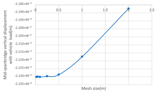
Figure 1. The convergence of mesh size on the mid-span bridge vertical displacement.

The vehicle was modeled as a 1 m block with a rectangular cross-section of 1 × 1 m. The density of the material is 5707 kg/m³, which leads to the mass of the vehicle equal to 5707 kg. The Young’s modulus is 2.87 × 10¹¹ Pa. Since the vehicle was modeled as a mass-sprung system, the vehicle block was kept short to avoid its vibration modes.

The vehicle model tire was simulated as a point mass, which is a rigid body with an assigned mass of 1 kg. The vehicle mass part was set 1 m above the bridge’s left end to assemble the model. The tire point has the same coordinate as that of the left end point of the bridge. A spring that has a stiffness of k = 0.5 × 10⁷ N/m was connected between the mid-point of the vehicle mass and the tire. To correctly model the vehicle–bridge interaction, the bridge part and the tire have a hard and surface-to-point contact. The bridge’s boundary conditions are set like this: the left end was pin supported and the right end was roller supported, with a restraint on the vertical displacement. All these settings were set in the initial step of the ABAQUS model [23].

In the second step, a gravity load was added onto the vehicle mass part. Static analysis was conducted thereafter, which simulates the vehicle gravity load on the model.

In the third step, the vehicle mass and tire parts were applied with a 27.7 m/s horizontal velocity. A dynamic, implicit analysis was performed to simulate the vehicle–bridge interaction along the whole bridge.

After completing the analysis, the mid-point vertical displacement of the bridge was extracted and compared with the literature results [24]. The comparison is shown in Figure 2.

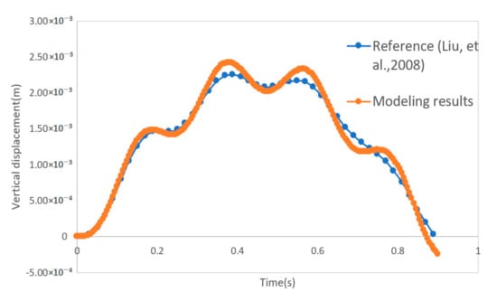
Figure 2. Comparison of mid-point displacements of the 2D vehicle–bridge interaction (VBI) ABAQUS model with the model of Liu et al. [24].

Figure 2 shows that the ABAQUS modeling results are almost the same as the displacement result of the reference [24], with a maximum difference of 5.1%. The small difference may be caused by the ABAQUS contact model, which is different from the semi-analytical contact model adopted in Liu et al. [24].

3.1. Effect of Damage on Bridge Frequencies

To compare the effects of different damages on the bridge, 12 damage models shown in Table 1 are analyzed.

Table 1. List of damaged model conditions.

Model #	Damage Location	Young’s Modulus	Damage Size
1, 2, 3	1 m	20% loss	0.1 m, 0.5 m, 1 m
4, 5, 6	5 m	20% loss	0.1 m, 0.5 m, 1 m
7, 8, 9	10 m	20% loss	0.1 m, 0.5 m, 1 m
10, 11, 12	12.5 m	20% loss	0.1 m
		40% loss
		60% loss

Three damage factors were simulated in the model: damage location, damage intensity, and damage size. Three different damage locations, damage intensities, and damage sizes were simulated in the model.

A healthy bridge of the example [24] was simulated first. A time step of 0.001 s was selected to generate adequate data. The time history of the vehicle’s vertical acceleration was recorded and shown in Figure 3. Three frequencies are successfully extracted from the Fast Fourier Transform (FFT) analysis of the vehicle’s vertical acceleration (Figure 4).

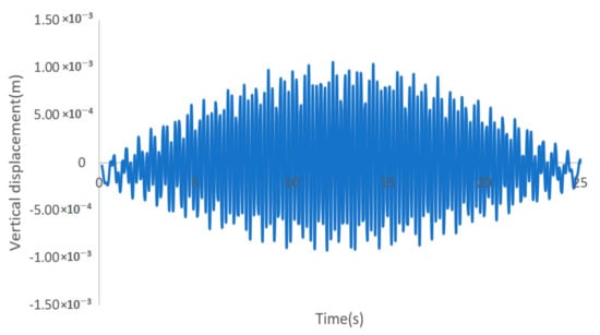
Figure 3. Vertical acceleration history of the vehicle.

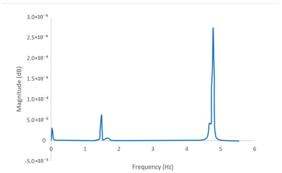
Figure 4. Fast Fourier transform of the bridge’s vertical acceleration.

In the frequency spectrum plot (Figure 4), the bridge frequency is about 4.76 Hz, the vehicle frequency is about 1.48 Hz, and the driving frequency is about 0.04 Hz. The three frequencies match well with the results of Liu et al. [24].

Based on the validated healthy bridge model, the above-mentioned damage cases are embedded in the model and simulated. Three model cases are created to study the effect of different damage locations, which are at the location of 1, 5, and 10 m from the bridge’s left end. The damage was simulated as a 1 m long segment in the bridge with half Young’s modulus of other elements. Other properties are kept the same as before. The simulated vertical acceleration data of the vehicle were recorded and used to extract the frequencies. The first frequency of the bridge with damage at 10, 5, and 1 m is 4.6, 4.68, and 4.76 Hz, respectively (Figure 5). The results show that the decrease of bridge frequency has a linear relationship concerning the distance between the support and the damage location. For damages close to the support, the resulted frequency does not change compared to that of the healthy bridge. This is reasonable since the damage close to support does not largely affect the bridge’s global stiffness compared to the damages in the center of the bridge.

Figure 5. Fast Fourier transform results in different damage locations.

A symmetric damage pattern was also simulated. The results show that if the damage location is symmetrical about the mid-span of the bridge. The identified frequency would be the same.

Another three model cases were created to study the effect of different damage levels. The Young’s modulus of a 1 m long segment of the bridge at the 10 m location from the left support is reduced by 20%, 40%, and 60% compared to its original Young’s modulus. Young’s modulus’ nominal variation could reflect the stiffness reduction caused by either section loss or material degradation. The identified first frequency of the bridge is 4.72, 4.64, and 4.52 Hz, respectively.

Four damage sizes at each damage location were simulated to study the vehicle responses’ sensitivity to damage sizes. The damage was still being simulated as only having half the Young’s modulus as these of other elements. The damage sizes were chosen as 1 m, 50 cm, and 10 cm, respectively.

At the 1 m damage location, the sensitivity of the damage size is very low. It is apparent that only the amplitude of the frequency spectrum changes, but not the frequency value.

At the 5 m damage location, the identified bridge frequency for the damaged bridge with a 1 m, 50 cm, and 10 cm length damage is 4.68, 4.72, and 4.76 Hz, respectively. It could be found that the identified bridge frequency reduces as the length of the damage segment increases.

At the 10 m damage location, the bridge’s identified frequency with the 1 m, 50 cm, and 10 cm length damage is 4.6, 4.68, and 4.86 Hz, respectively. A similar trend is found in the case of damage at the 5 m location.

3.2. Short Time Fourier Transform Results

Short-Time Fourier Transform (STFT) analysis is an advanced signal processing method that allows the frequency spectrum to change with time.

The effect of different window sizes was researched first. Five different window sizes are selected: 10, 20, 50, 100, and 200, respectively. The STFT of vertical accelerations of the vehicle driving on the health bridge is shown for window size of 100 and 200 in Figure 6 and Figure 7. Here window size means how many time data will be processed at each time instant, and STFT will swipe-process the complete data set through FFT analysis of each segmented window. Through STFT, local disturbance in the time history data could be revealed.

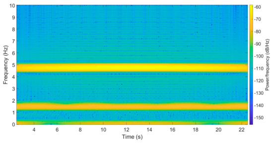
Figure 6. Short-time Fourier transformation of the healthy bridge accelerations with window size 100.

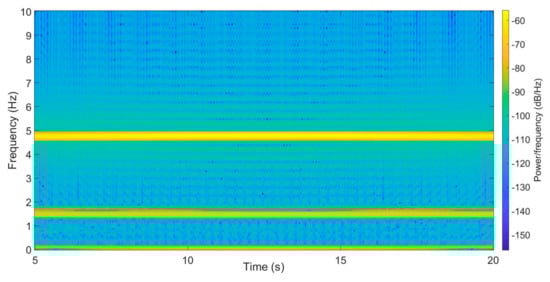
Figure 7. Short-time Fourier transformation of the healthy bridge accelerations with window size 200.

Figure 6 and Figure 7 show that the STFT results with a larger window will get better resolution. However, the results of STFT will lose some data at the beginning and ending of the signal equal to half the number of the window length. In other words, more data will be lost with a larger window. As for this research, the rest study will use a window size of 100.

When damage exists, the STFT results will show that some area’s color is changed, which means the frequency energy of indicated areas is changed. Figure 8 presents the results of the 1 m length damage at 5 m location.

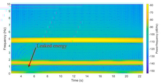
Figure 8. Short-time Fourier transformation of the bridge accelerations with damage at 5 m location.

All damaged cases show similar changing patterns: the low-frequency range energy will increase due to the energy leaked from the original frequency bands at different locations. In this way, the energy of frequency ranging from 0.39 to 1.10 Hz was analyzed to find the relationship between the STFT results and different damage cases.

To identify the damage location, a basic energy line was set from the healthy bridge results (Figure 6). The average energy of the aimed range frequency is −113.08 dB/Hz, and it could be assumed that if a 5% change to the energy happens, the location could be marked as a damaged area. As for this study, the identified damaged area starts when the average energy becomes constantly larger than −107.7 dB/Hz.

The mid locations of damaged areas are compared between real cases and identified results for different damage locations and shown in Table 2.

Table 2. Comparison of Short-Time Fourier Transform (STFT) results of different damage locations on the bridge.

Cases	Real Mid Location(m)	Identified Results
		Start Location (m)	End Location (m)	Mid Location (m)	Ave Energy (dB/Hz)
1 m damage at 1 m location	1.5	2.5	3.45	2.975	−101.06
1 m damage at 5 m location	5.5	3.25	7.85	5.55	−97.234
1 m damage at 10 m location	10.5	8.05	12.95	10.5	−95.321

Table 2 shows that the damage locations identified are close to the real cases at 5 m and 10 m. For the 1 m damage location case, 50 data (2.5 m long) are lost due to the STFT analysis, leading to the not-so-accurate damage identification.

The mid locations of damaged areas and damaged lengths are compared between the real sizes and the identified results for different damage sizes.

Table 3 shows that for different size damages, damage location identification still works fine. However, the identified damage sizes are not consistent with the real sizes. The chosen basic energy line may cause this.

Table 3. Comparison of STFT results of bridges with different damage sizes.

Cases	Real Mid Location(m)	Real Damaged Length(m)	Identified Results
			Start Location(m)	End Location(m)	Mid Location(m)	Damaged Length (m)	Ave Energy (dB/Hz)
1 m damage at 10 m location	10.5	1	8.05	12.95	10.5	4.9	−95.321
0.5 m damage at 5 m location	10.25	0.5	8.05	12.4	10.225	4.35	−93.278
0.1 m damage at 10 m location	10.05	0.1	8.5	11.6	10.05	3.1	−101.667

For different damage levels, only the energy zone at the damaged area is analyzed. The damaged area is at the 10 to 11 m location of the bridge. The energy change with respect to different damage levels is summarized and shown in Figure 9.

Figure 9. Comparison of STFT results of bridge accelerations with different damage levels.

Figure 9 shows that the damage area’s energy loss has a linear relationship with the damage level, which could be used to identify the damage level once the STFT spectrum of the vertical vehicle acceleration is generated.

For multiple damages, 1 m damages are set at the 5, 10, and 20 m locations; the results of STFT on the vertical vehicle acceleration is shown in Figure 10.

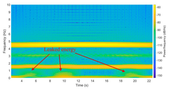
Figure 10. Comparison of STFT results of bridge accelerations with multiple damages.

Figure 10 showed that for multiple damages, the STFT method can still work. Changes of frequencies and energy leaked at the damage zones can be identified according to the damage locations.

4. Drive-By Inspection through 3D Virtual Simulations

Following a previous study [22,25], a 3D vehicle model based on a real truck HS20-44 was created. The model uses the same vehicle properties as Oliva et al. [25] did, including mass, spring stiffness, damping, and body rotary inertias. The needed vehicle parameters are shown in Figure 11. Its specific parameters are given in Table 4. The first seven natural frequencies and relative mode shapes are extracted and compared in ABAQUS (Figure 12).

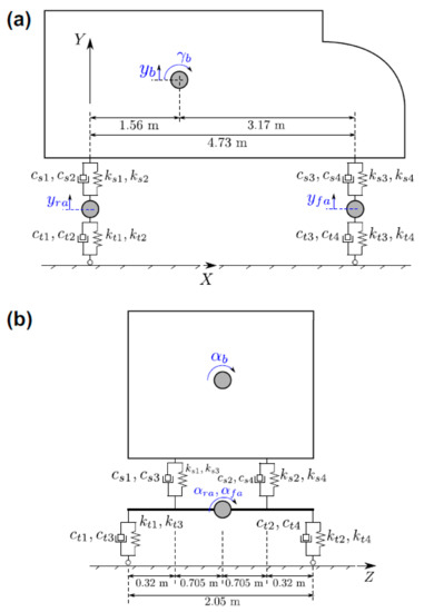
Figure 11. Truck model: (a) side view, (b) rear view.

Table 4. The mechanical parameters of the vehicle.

Element	Notation	Value
Stiffness(N/m)
Rear wheels	Kt1, kt2	1.57 × 106
Front wheels	Kt3, kt4	7.85 × 105
Rear suspensions	Ks1, ks2	3.73 × 105
Front suspension	Ks3, ks4	1.16 × 105
Dampings (N*s/m)
Rear wheels	Ct1, Ct2	200
Front wheels	Ct3, Ct4	100
Rear suspensions	Cs1, Cs2	35,000
Front suspension	Cs3, Cs4	25,000
Masses (Kg)
Rear axle	mra	1000
Front axle	mfa	600
Body	mb	17,000
Rotatory Inertias (kg*m2)
Rear axle (roll)	Iα,ra	600
Front axle (roll)	Iα,fa	550
Body (roll)	Iα,b	13,000
Body (pitch)	Iγ,b	90,000

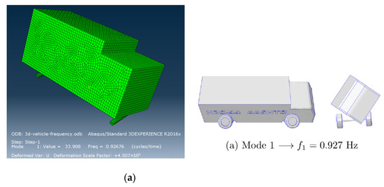
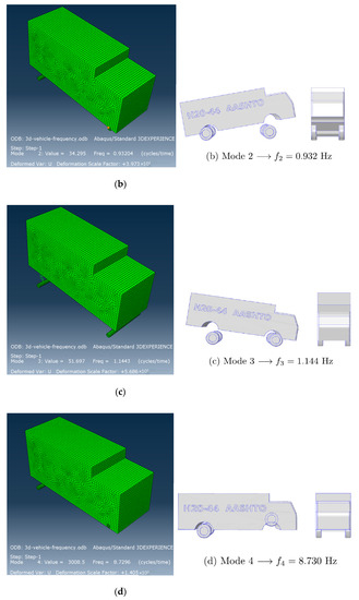
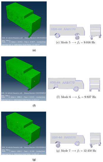
Figure 12. Comparison of the model vehicle frequencies with the literature results. (a) Model 1, (b) Model 2, (c) Model 3, (d) Model 4, (e) Model 5, (f) Model 6, and (g) Model 7.

In the ABAQUS model, all truck bodies are assumed rigid and modeled using element type R3D4 with a mesh size of 0.1 m, since the vibration caused by external forces is concerned, and the deformation of the truck body itself is small and could be neglected. The rigid body needs to have a reference point, which is set as the geometry center of each part.

The rotatory inertias are attached to the reference point of the body part. However, the axle parts could not simply attach the mass and rotatory inertia on the reference point since this will make the axle only have vertical displacement but no rotation. In solving this issue, the axle mass is divided into four-point masses, and the locations can be calculated to meet the given rotatory inertia. Through these implementations, the ABAQUS truck model’s frequency analysis results are quite the same as those by Oliva et al. [25]. Comparing these frequencies in Oliva et al. [25], the current results are shown in Figure 12.

A 3D multiple-span bridge was also created based on previous research [22] and used to test the drive-by inspection hypothesis. Shell element type S4R was adopted. The bridge is 79.2 m long in total, with three 26.4 m spans. The width is 10.7 m, and the depth is 0.95 m. Young’s modulus is 14.54 × 10¹⁰ N/m², Poisson’s ratio is 0.3, and the density of the bridge material is 2375 kg/m³. The vehicle crosses the bridge with its right tires at a distance of 1 m from the bridge’s right span edge.

The bridge’s left boundary is fixed, while the two intermediate supports and the right boundary only have the lateral movement allowed. A similar mesh size sensitivity study was conducted and shown in Figure 13. The results suggest that mesh size under 0.1 is adequate and convergent in capturing bridge displacement. In the later simulations of this model, 0.1 m was chosen as the mesh size.

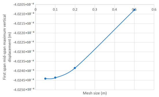
Figure 13. Mesh sensitivity plot for the three-span bridge.

The first mid-span vertical displacement results are recorded and compared with the literature results [22] in Figure 14, when the truck passes the bridge with a speed of 32.0 m/s.

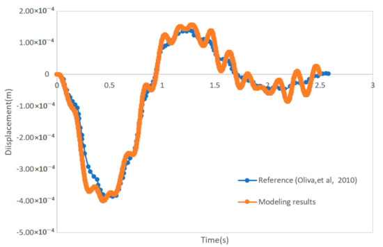
Figure 14. The mid-span displacement time history of the first span when the truck passes at 32.5 m/s.

Figure 14 shows that the numerical model captures the bridge and vehicle interaction quite accurately. The small oscillations from the current model may be caused by higher frequencies of bridge, vehicle, or the interaction between vehicle and bridge in the present model since a smaller time step is adopted.

4.1. Bridge Frequencies Detection through Vehicle Responses

When vehicle speed decreases to 1 m/s, the FFT results of the vehicle front body accelerations can be used to identify frequencies of the truck and the bridge.

Using the vehicle vertical acceleration data collected from the front tire, bridge frequency values can be identified, shown in Figure 15 and Table 5.

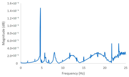
Figure 15. Identified frequencies using the front tire acceleration time history.

Table 5. Identified bridge frequencies through the front tire acceleration time history.

	Reference Bridge Frequencies (Hz)
	4.83	6.21	9.13	16.23	17.24	18.57	18.91	20.94
FFT Results	4.65	6.65	10.00	16.65		18.45		20.00

Table 5 shows that most bridge frequencies can be identified through the FFT results of the vehicle’s vertical acceleration.

4.2. STFT of Vehicle Responses and Its Relationship with Damage

To demonstrate the effectiveness of STFT in 3D bridge damage detections, a simply supported short bridge was used to filter out the effect of internal supports. The bridge has the properties shown in Table 6.

Table 6. Properties of the simulated short bridge.

Length	15 m	Young′s Modulus	3E10 N/m2
Width	10 m	Poisson’s modulus	0.2
Thickness	1 m	Density	2500 Kg/m3
Damping	2%

When the tire moves on the damaged bridge, the vehicle’s vibration will be changed, which would cause the STFT results to show multiple high energy frequencies between 20 Hz to 50 Hz (Figure 16) between 0–7 s. Similar changes will occur when the front tire drives out of the bridge or the rear tire drives in the bridge. The acceleration data were collected from the rear tire because the frequency changes caused by the front tire driving out the bridge are smaller than those caused by the rear tire on the damaged bridge. The underlying reason could be explained as the front tire acts as an actuator while the rear tire acts as a sensor to pick up the signal excited and accumulated through time.

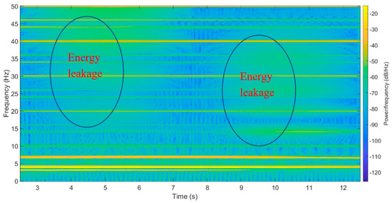
Figure 16. STFT result of the bridge deck with a 10 cm damage at 5 m through the drive-by front tire acceleration time history (Energy leaked zones).

A 10% energy difference of the frequency range between 47 Hz to 50 Hz is set as the threshold for damage identification to identify the damage.

To simulate different damage locations, a 10 cm segment with 80% original Young’s modulus was set to 5.0, 7.5, and 10 m of the bridge. The predicted locations are listed in Table 7 for comparison.

Table 7. Comparison of the predicted and real damage locations.

Cases	Real Mid Location(m)	Identified Results
		Start Location (m)	End Location (m)	Mid Location (m)	Error (m)	Aver. Energy (dB/Hz)
0.1 m damage at 5 m location	5.05	4.81	5.3	5.05	0	−88.06
0.1 m damage at 7.5 m location	7.55	7.21	7.85	7.53	0.02	−87.73
0.1 m damage at 10 m location	10.05	9.05	10.95	10.0	0.05	−106.87

Table 7 shows that the damage location has been identified successfully through the vehicle’s vertical acceleration history.

To reflect the effect of the damage severities, a 10 cm segment with 20%, 40%, and 60% loss of original Young’s modulus was set at 7.5 m. The change of frequency energy can be plotted with the modulus loss, as shown in Figure 17.

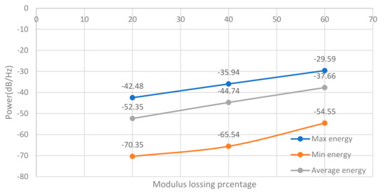
Figure 17. STFT energy results for different damage levels.

Figure 17 shows that the energy change for each spectrum frequency has a linear relationship with the bridge deck’s damage level.

5. Effect of Road Roughness on Drive-By Bridge Inspection

According to the ISO standard 8608, road surface profiles can be represented with a zero-mean normal stationary ergodic random process described by their Power Spectral Density. The following function (Equation(1)) can describe the PSD:

$$G\left(n\right)=G\left(n_0\right){\left(\frac{n}{n_0}\right)}^{-2}.$$

(1)

The G(n) is the power spectral density for the spatial frequency n and G(n₀) is the power spectral density for the reference spatial frequency n₀ = 0.1 m⁻¹. The value of G(n₀) represents the road profile class, as shown in Table 8.

Table 8. Road roughness classification.

Road Class	G(n0) (m3)
A (very good)	1.600 × 10−5
B (good)	6.400 × 10−5
C (medium)	2.560 × 10−4
D (poor)	1.024 × 10−3
E (very poor)	4.096 × 10−3

Road profiles could be generated as the sum of a series of harmonics (Equation (2)):

$$y_1\left(x\right)={\displaystyle \sum }_i^N\sqrt{2G\left(n_i\right)\Delta n}cos\left(2\pi n_{i}x+{\varnothing }_i\right)$$

(2)

where ϕ_i is the random phase angle uniformly distributed from 0 to 2π. This expression employs N frequencies between two values n_min and n_max and the increment value (Δn) is defined as Equation (3),

$$\Delta n=\frac{n_{max}-n_{min}}{N}$$

(3)

In this study, Class B road profile was chosen to be simulated in the 3D VBI model. The profile was generated through Matlab, then written into the 3D bridge model through the ABAQUS input file. The steps used in road roughness generation could be summarized as follows:

• Establish the original bridge in ABAQUS, and generate an input file of the model;
• Generate a 2D roughness profile in the ABAQUS with the same node points as the ABAQUS bridge model. The profile is generated line by line in the vehicle moving direction using Equation (2). Each line is different from the other, but the trend of each line is the same.
• Reshape the roughness amplitude matrix into one column and replace the node coordinate inputs in the ABAQUS input file with the generated roughness node coordinates.

Figure 18 shows a generated road roughness from Matlab for a class B road roughness. Figure 19 shows the power spectrum density (PSD) plot of the generated roughness, which displays a fitted linear relationship between spatial frequencies and roughness profile PSDs with a fitting coefficient close to −2. The −2 slope obtained verifies Equation (1) and the road profile generated.

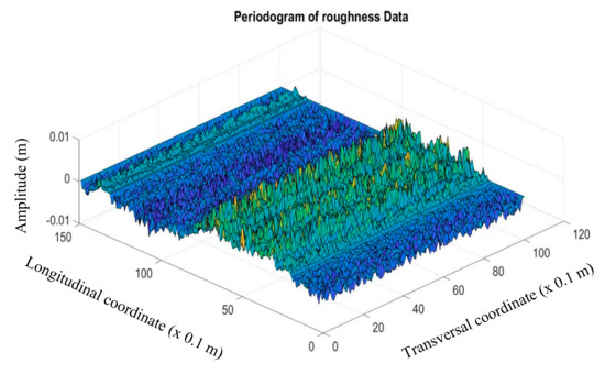
Figure 18. Class B road roughness generated.

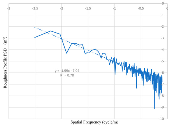
Figure 19. Roughness profile PSDs versus spatial frequencies.

5.1. Effect of Roughness on Initial Conditions of VBI interaction Simulations

Initial vehicle status can affect the detection of bridge properties, which has been verified by Y. B. Yang [1]. To find how the road roughness affects vehicle status, a series of model simulations are conducted.

A 30 by 10 m ground was generated in ABAQUS. It has the same property as the short bridge. The vehicle will drive through the ground in 10, 20, 25, and 30 m/s with four different offset distances with the bridge entrance. The displacement, velocity, and acceleration amplitude of the vehicle when entering the bridge will be compared. Four plots of the right front axle acceleration history of the vehicle are shown in Figure 20, Figure 21, Figure 22 and Figure 23.

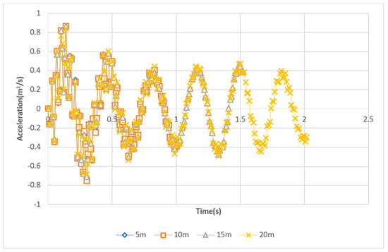
Figure 20. Right front axle acceleration history when approaching the bridge at 10 m/s.

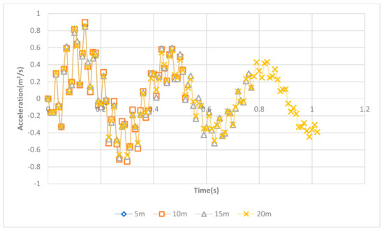
Figure 21. Right front axle acceleration history when approaching the bridge at 20 m/s.

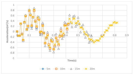
Figure 22. Right front axle acceleration history when approaching the bridge at 25 m/s.

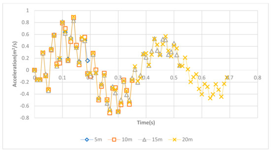
Figure 23. Right front axle acceleration history when approaching the bridge at 30 m/s.

FFT Results of the vehicle acceleration responses when driving from a 20 m offset distance with a speed of 10 m/s is shown in Figure 24, which shows that there are two acceleration vibration frequencies. One frequency is at 3 Hz, while the other one is at 28 Hz. Their corresponding amplitudes at different driving distances for the two-frequency component are shown in Table 9 and Table 10.

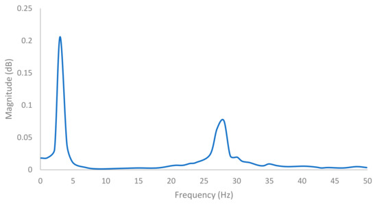
Figure 24. FFT results of the vehicle acceleration responses when driving from a 20 m offset distance with a speed of 10 m/s.

Table 9. Acceleration amplitude for the 3 Hz component in the vehicle’s vibration.

		Driving Distance
		5 m	10 m	15 m	20 m
Driving Speed	10 m/s	0.393	0.384	0.423	0.312
	20 m/s	0.491	0.412	0.373	0.377
	25 m/s	0.511	0.498	0.384	0.341
	30 m/s	0.518	0.508	0.386	0.352

Table 10. Acceleration amplitude for the 28 Hz component in the vehicle’s vibration.

		Driving Distance
		5 m	10 m	15 m	20 m
Driving speed	10 m/s	0.14	0.036	0.003	0.021
	20 m/s	0.202	0.124	0.103	0.07
	25 m/s	0.285	0.211	0.121	0.019
	30 m/s	0.334	0.266	0.123	0.116

From the two amplitude results, the vibration of the vehicle keeps decreasing with longer driving distance. This decrease is caused by the damping of the vehicle. Furthermore, with the driving speed increasing, the ending amplitude becomes larger. This is because the damping of the vehicle does not have enough time to release the energy. However, to simulate a VBI model accurately, it is important to set adequate driving distance from the bridge’s entrance. Otherwise, additional frequencies will be included in the model and affect the simulation accuracy. From the above simulations, 10 m offset distance is needed for speed less than 20 m/s, 15 m offset distance is needed for speed between 20–25 m/s, while more than 20 m offset distance is needed for speed at 30 m/s and above.

5.2. Road Roughness and Bridge Frequency

Using the same method, the Class B road profile can be added to the short bridge surface. The vehicle is driven through the bridge at a speed of 1 m/s. As the rear axle goes through the bridge’s whole length, the acceleration data were collected from the right rear axle.

The FFT process of the collected acceleration data from the right rear axle is shown in Figure 25.

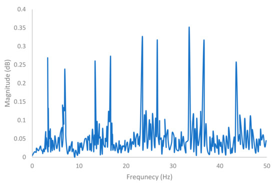
Figure 25. FFT of right rear axle acceleration history of the VBI model on the bridge with the generated road roughness.

The comparison of identified results and reference bridge frequencies are listed in Table 11.

Table 11. Comparison of identified bridge frequencies and the theoretical bridge frequencies (Hz).

	Bridge Frequencies
Theoretical bridge frequency		7		15.4		28		38.6
Identified frequency	3.4	6.94	13.4	16.6	23.4	26.6	33.4	36.6	43.4

From Table 11, we could see the drive-by inspection could identify most of the bridge frequencies.

5.3. Effect of Road Roughness on STFT Damage Detection

After the road roughness was superimposed onto the bridge deck, a test of damage detection was conducted through the 3D VBI model with embedded damages. Its STFT results are shown in Figure 26, Figure 27, Figure 28, Figure 29 and Figure 30.

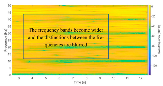
Figure 26. STFT results of right rear axle acceleration history of the vehicle on undamaged bridges with the given roughness.

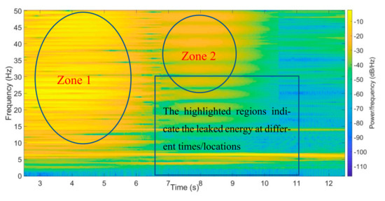
Figure 27. STFT results of vehicle’s right rear axle acceleration difference between the 40% damage case and the healthy bridge.

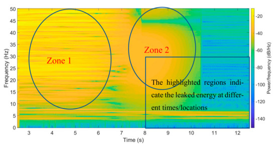
Figure 28. STFT results of vehicle’s right rear axle acceleration difference between the 60% damage case and the healthy bridge.

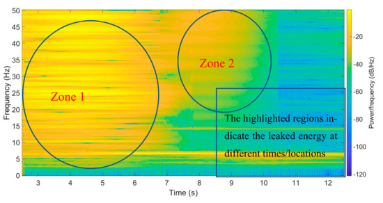
Figure 29. STFT results of vehicle’s right rear axle acceleration difference between the 80% damage case and the healthy bridge.

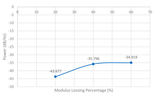
Figure 30. Average PSD energy over the damaged area (7.5 m to 7.6 m).

The STFT results show that there is much roughness noise signal. To reduce the effect of roughness, the vibration differences between the healthy bridge and damaged bridge were used to process the STFT analysis results. A 0.1 m damage with 40%, 60%, and 80% of the original Young’s modulus was set at the bridge’s mid-span.

In these three plots, the acceleration differences can not completely offset all roughness effects. However, the frequencies between 20 to 50 Hz have obvious changes at 7.5 m according to different damage levels (Figure 30). The STFT method still can identify different damages of bridges with consideration of the roughness effect.

6. Summary and Conclusions

Based on the series of 2D and 3D virtual VBI simulations conducted in this study, the following conclusions are derived:

• FFT of vehicle accelerations during drive-by inspection can capture bridge frequencies accurately. In the 2D VBI model, the captured frequencies can reflect the damage with a decrease in their magnitudes. In the 3D VBI model, the FFT method can capture most frequencies of multiple span bridges with high accuracy, even with damages included.
• STFT method works well in identifying damages through drive-by vehicle responses in the VBI models. Energy change in STFT results of drive-by vehicle responses can identify the damage location and the damage level in high accuracy.
• Vibration caused by roughness affects the initial entering conditions of vehicles in the VBI models. The offset distances of the vehicle before entering the bridge are found to ensure the accurate bridge and vehicle responses through VBI simulations, which requires a 10 m offset distance for speed less than 20 m/s, a 15 m offset distance for speed between 20–25 m/s, and more than 20 m offset distance is needed for speed over 30 m/s for a class B road profile.
• Roughness increases the difficulty in identifying bridge damages through drive-by vehicle responses. However, the STFT method still has the capability of detecting damage levels and damage location in bridges.

References

- Yang, Y.-B.; Lin, C.W.; Yau, J.D. Extracting bridge frequencies from the dynamic response of a passing vehicle. J. Sound Vib. 2004, 272, 471–493. [Google Scholar] [CrossRef]
- Yang, Y.-B.; Lin, C.W. Vehicle-bridge interaction dynamics and potential applications. J. Sound Vib. 2005, 284, 205–226. [Google Scholar] [CrossRef]
- Yang, Y.-B.; Lin, C.W. Use of a passing vehicle to scan the fundamental bridge frequencies: An experimental verification. Eng. Struct. 2005, 27, 1865–1878. [Google Scholar] [CrossRef]
- Yang, Y.-B.; Chang, K.C. Extracting the bridge frequencies indirectly from a passing vehicle: Parametric study. Eng. Struct. 2009, 31, 2448–2459. [Google Scholar] [CrossRef]
- Yang, Y.-B.; Li, Y.C.; Chang, K.C. Constructing the mode shapes of a bridge from a passing vehicle: A theoretical study. Smart Struct. Syst. 2014, 13, 797–819. [Google Scholar] [CrossRef]
- González, A.; Covian, E.; Madera, J. Determination of bridge natural frequencies using a moving vehicle instrumented with accelerometers and GPS. In Proceedings of the Ninth International Conference on Computational Structures Technology (CST), Athens, Greece, 2–5 September 2008. [Google Scholar] [CrossRef]
- González, A.; OBrien, E.; McGetrick, P. Detection of bridge dynamic parameters using an instrumented vehicle. In Proceedings of the Fifth World Conference on Structural Control and Monitoring (5WCSCM), Tokyo, Japan, 12–14 July 2010. [Google Scholar]
- Zhang, Y.; Wang, L.; Xiang, Z. Damage detection by mode shape squares extracted from a passing vehicle. J. Sound Vib. 2012, 331, 291–307. [Google Scholar] [CrossRef]
- Malekjafarian, A.; OBrien, E.J. Identification of bridge mode shapes using short time frequency domain decomposition of the responses measured in a passing vehicle. Eng. Struct. 2014, 81, 386–397. [Google Scholar] [CrossRef]
- Malekjafarian, A.; OBrien, E.J. A mode shape-based damage detection approach using laser measurement from a vehicle crossing a simply supported bridge. Struct. Control Health Monit. 2016, 23, 1273–1286. [Google Scholar] [CrossRef]
- Kong, X.; Cai, C.; Kong, B. Numerically extracting bridge modal properties from dynamic responses of moving vehicles. J. Eng. Mech. 2016, 142. [Google Scholar] [CrossRef]
- Kong, X.; Cai, C.; Deng, L.; Zhang, W. Using dynamic responses of moving vehicles to extract bridge modal properties of a field bridge. J. Bridge Eng. 2017, 22. [Google Scholar] [CrossRef]
- Shokravi, H.; Bakhary, N.; Heidarrezaei, M.; Rahimian Koloor, S.S.; Petru, M. A review on vehicle classification and potential use of smart vehicle-assisted techniques. Sensors 2020, 20, 3274. [Google Scholar] [CrossRef] [PubMed]
- Tan, C.; Uddin, N.; O’Brien, E.J.; McGetrick, P.J.; Kim, C.W. Extraction of bridge modal parameters using passing vehicle response. J. Bridge Eng. 2019, 24, 04019087. [Google Scholar] [CrossRef]
- Sitton, J.D.; Zeinali, Y.; Rajan, D.; Story, B.A. Frequency estimation on two-span continuous bridges under dynamic responses of passing vehicles. J. Eng. Mech. 2020, 146, 04019115. [Google Scholar] [CrossRef]
- Elhattab, A.; Uddin, N.; OBrien, E. Drive-by bridge frequency identification under operational roadway speeds employing frequency independent underdamped pinning stochastic resonance (FI-UPSR). Sensors 2018, 18, 4207. [Google Scholar] [CrossRef]
- Tan, C.; Elhattab, A.; Uddin, N. Wavelet entropy-approach-for-detection-of-bridge-damages-using-direct-and-indirect-bridge-recordsjournal-of-infrastructure-systems. J. Infrastruct. Syst. 2020, 26, 04020037. [Google Scholar] [CrossRef]
- Tan, C.; Uddin, N. Hilbert transform based approach to improve extraction of ‘drive-by’ bridge frequency. Smart Struct. Syst. 2020, 25, 265–277. [Google Scholar] [CrossRef]
- Kildashtia, K.; Makki Alamdari, M.; Kim, C.W.; Gaob, W.; Samalia, B. Drive-by-bridge inspection for damage identification in a cable-stayed bridge: Numerical investigations. Eng. Struct. 2020, 223, 110891. [Google Scholar] [CrossRef]
- Li, J.; Zhu, X.; Law, S.; Samali, B. A two-step drive-by bridge damage detection using dual kalman filter. Int. J. Struct. Stab. Dyn. 2020, 20, 2042006. [Google Scholar] [CrossRef]
- Sitton, J.D.; Rajan, D.; Story, B.A. Bridge frequency estimation strategies using smartphones. J. Struct. Health Monit. 2020, 10, 513–526. [Google Scholar] [CrossRef]
- Oliva, J.; Goicolea, J.M.; Antolín, P.; Astiz, M.Á. Relevance of a complete road surface description in vehicle-bridge interaction dynamics. Eng. Struct. 2013, 56, 466–476. [Google Scholar] [CrossRef]
- Abaqus/CAE User’s Guide, Simulia. 2018. Available online: http://130.149.89.49:2080/v6.14/pdf_books/CAE.pdf (accessed on 21 December 2020).
- Liu, X.W.; Xie, J.; Wu, C.; Huang, X.C. Semi-analytical solution of vehicle-bridge interaction on transient jump of wheel. Eng. Struct. 2008, 30, 2401–2412. [Google Scholar] [CrossRef]
- Oliva, J.; Goicolea, J.M.; Antolín, P.; Astiz, M.Á. Finite element models for dynamic analysis of vehicles and bridges under traffic loads. In Proceedings of the SIMULIA Customer Conference, Providence, RI, USA, 25–27 May 2010. [Google Scholar]
Publisher’s Note: MDPI stays neutral with regard to jurisdictional claims in published maps and institutional affiliations. |
© 2020 by the authors. Licensee MDPI, Basel, Switzerland. This article is an open access article distributed under the terms and conditions of the Creative Commons Attribution (CC BY) license (http://creativecommons.org/licenses/by/4.0/).