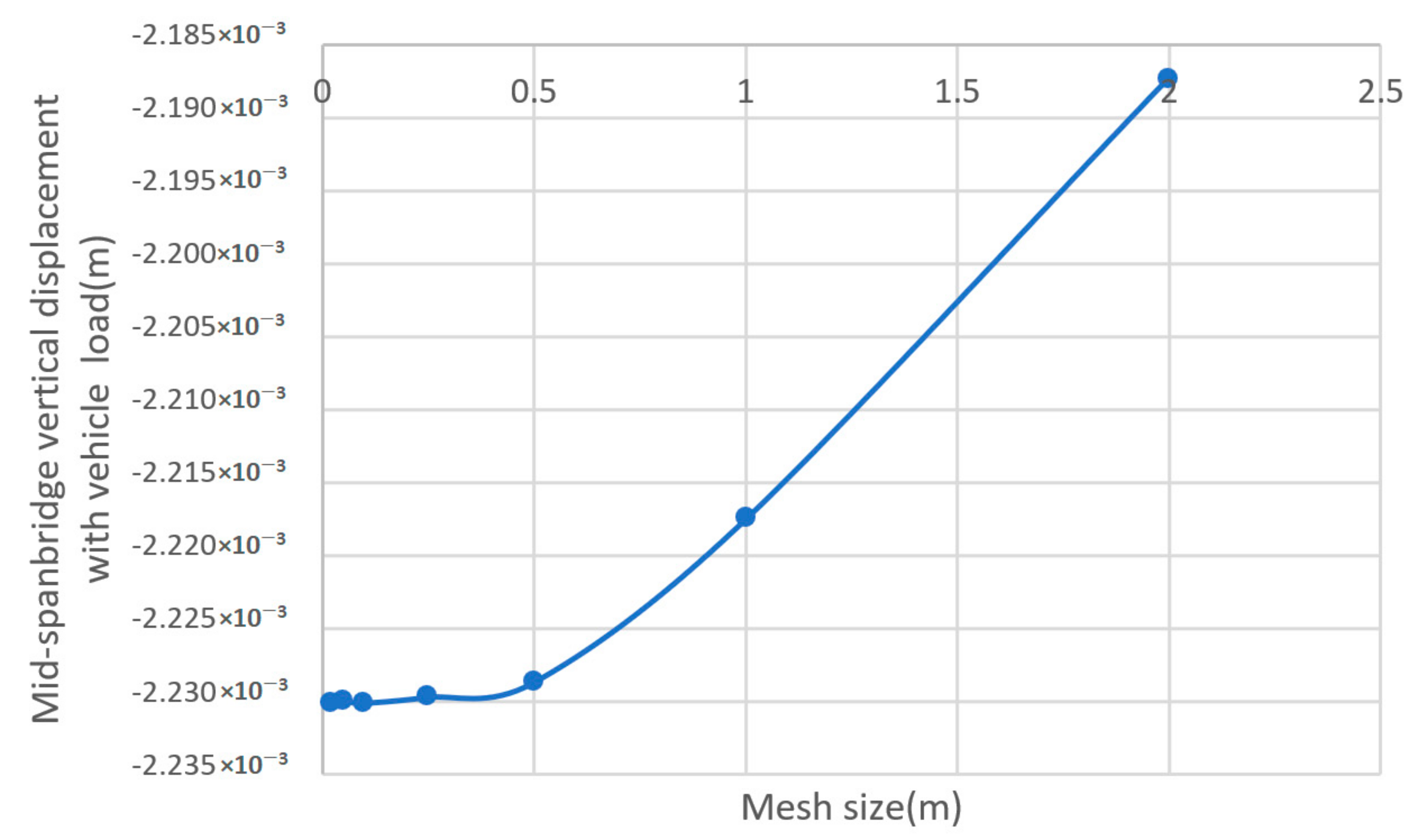
Figure 1.
The convergence of mesh size on the mid-span bridge vertical displacement.
Figure 1.
The convergence of mesh size on the mid-span bridge vertical displacement.
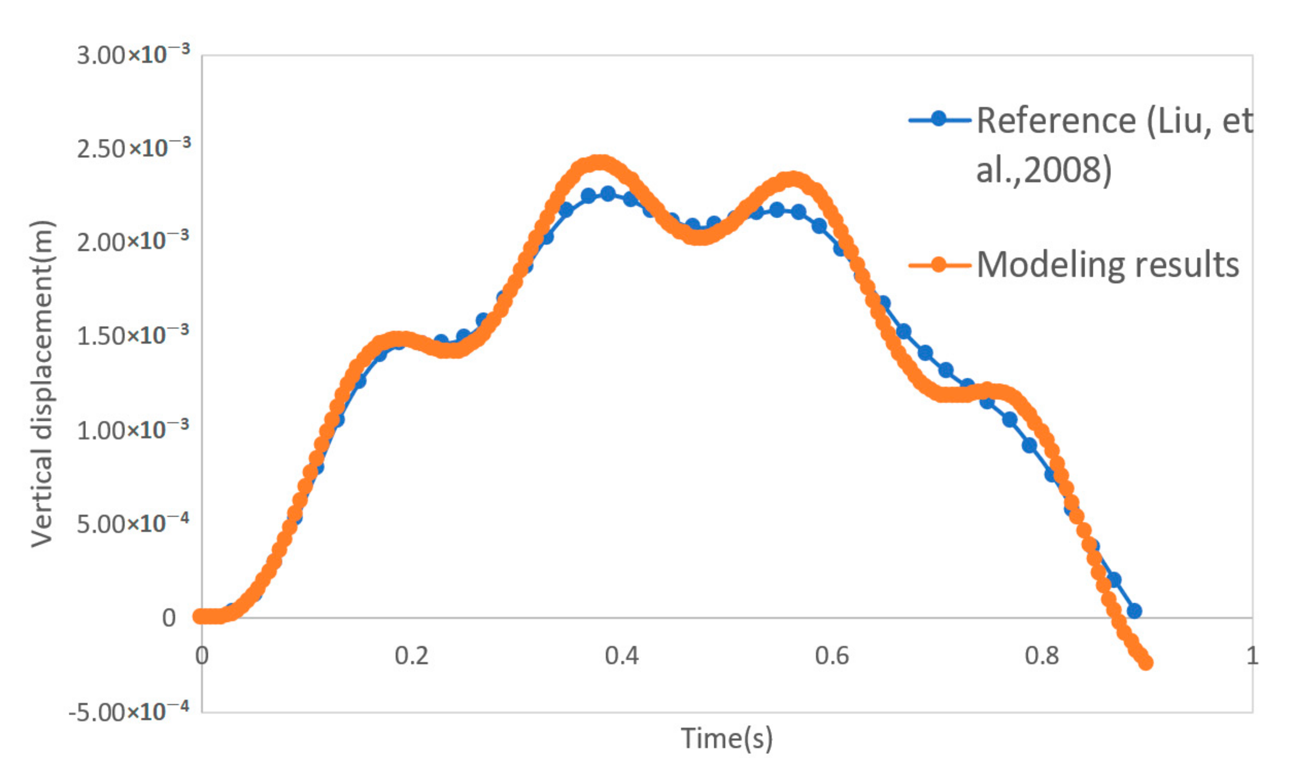
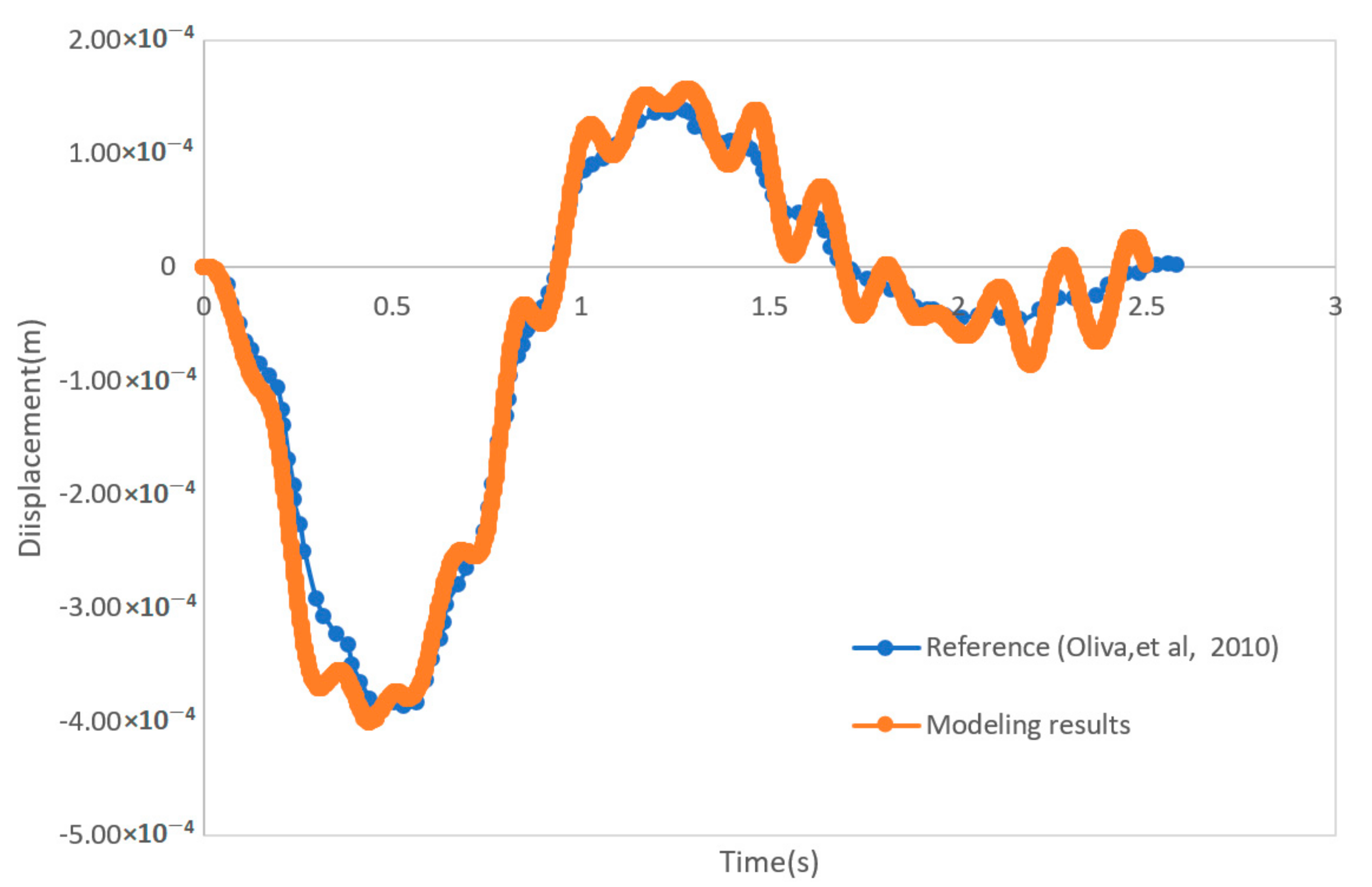
Figure 2.
Comparison of mid-point displacements of the 2D vehicle–bridge interaction (VBI) ABAQUS model with the model of Liu et al. [
24].
Figure 2.
Comparison of mid-point displacements of the 2D vehicle–bridge interaction (VBI) ABAQUS model with the model of Liu et al. [
24].
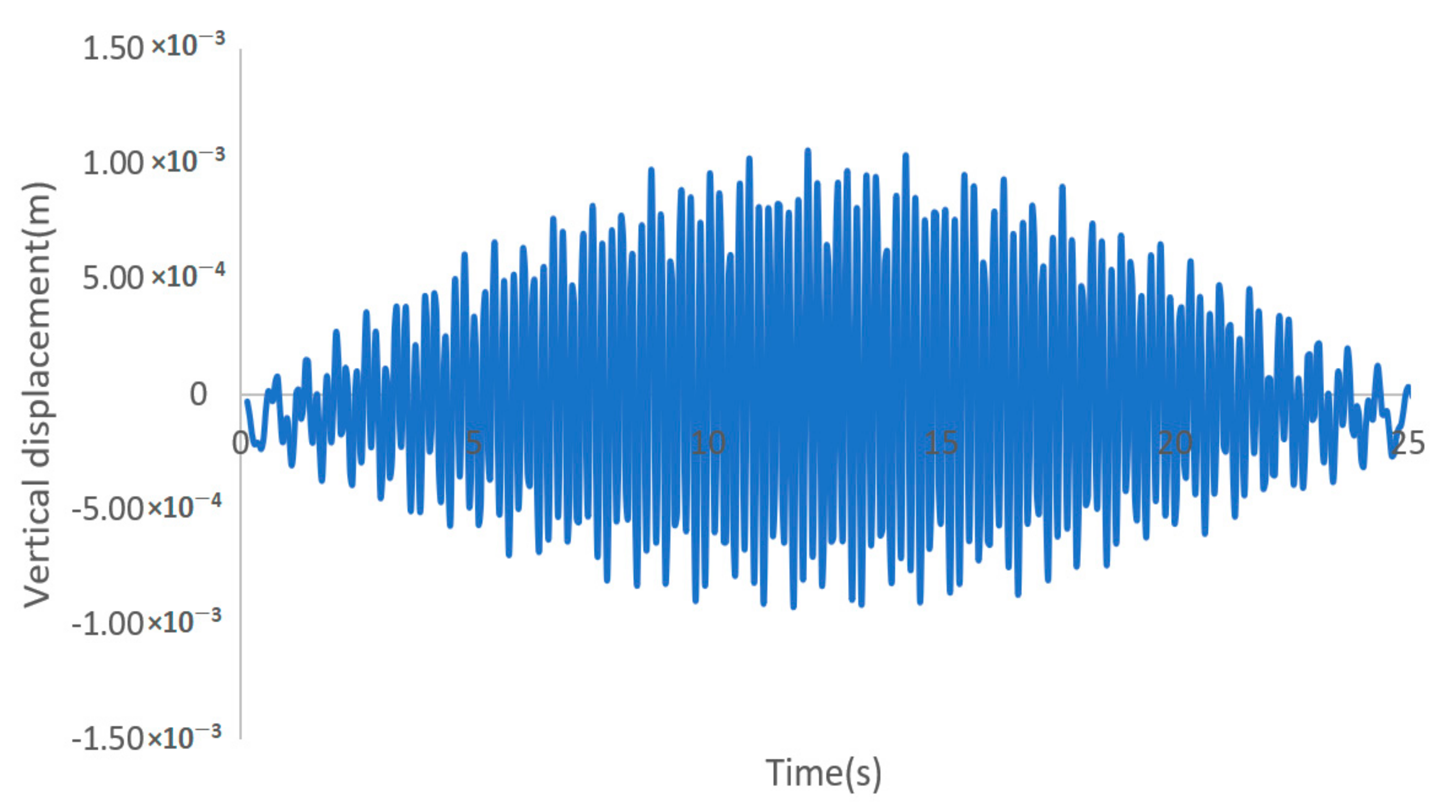
Figure 3.
Vertical acceleration history of the vehicle.
Figure 3.
Vertical acceleration history of the vehicle.
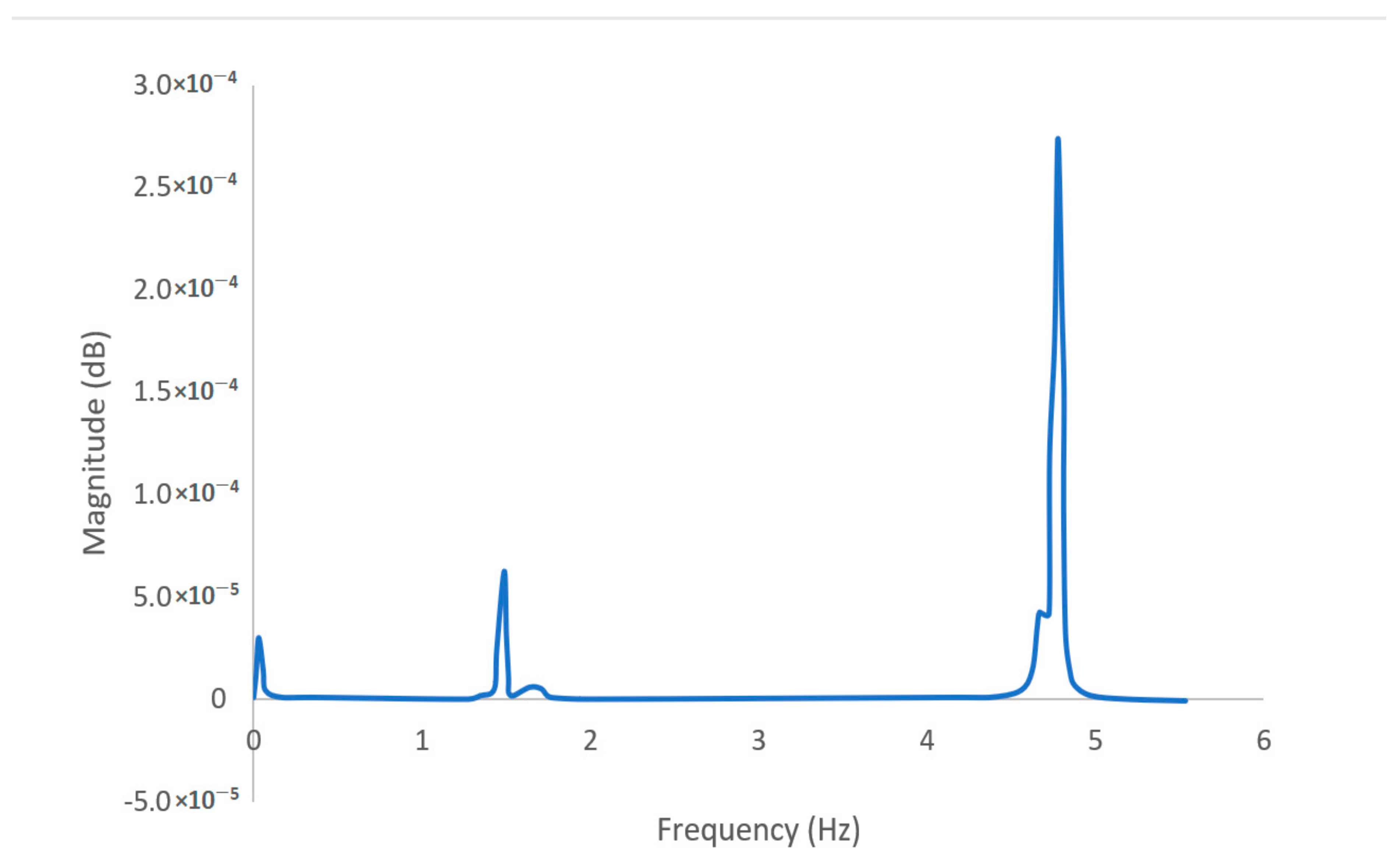
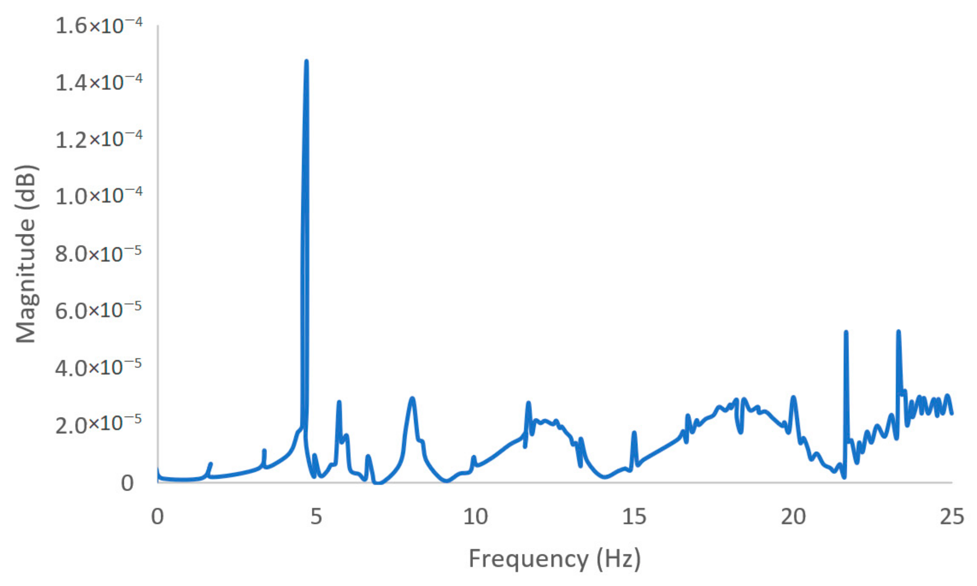
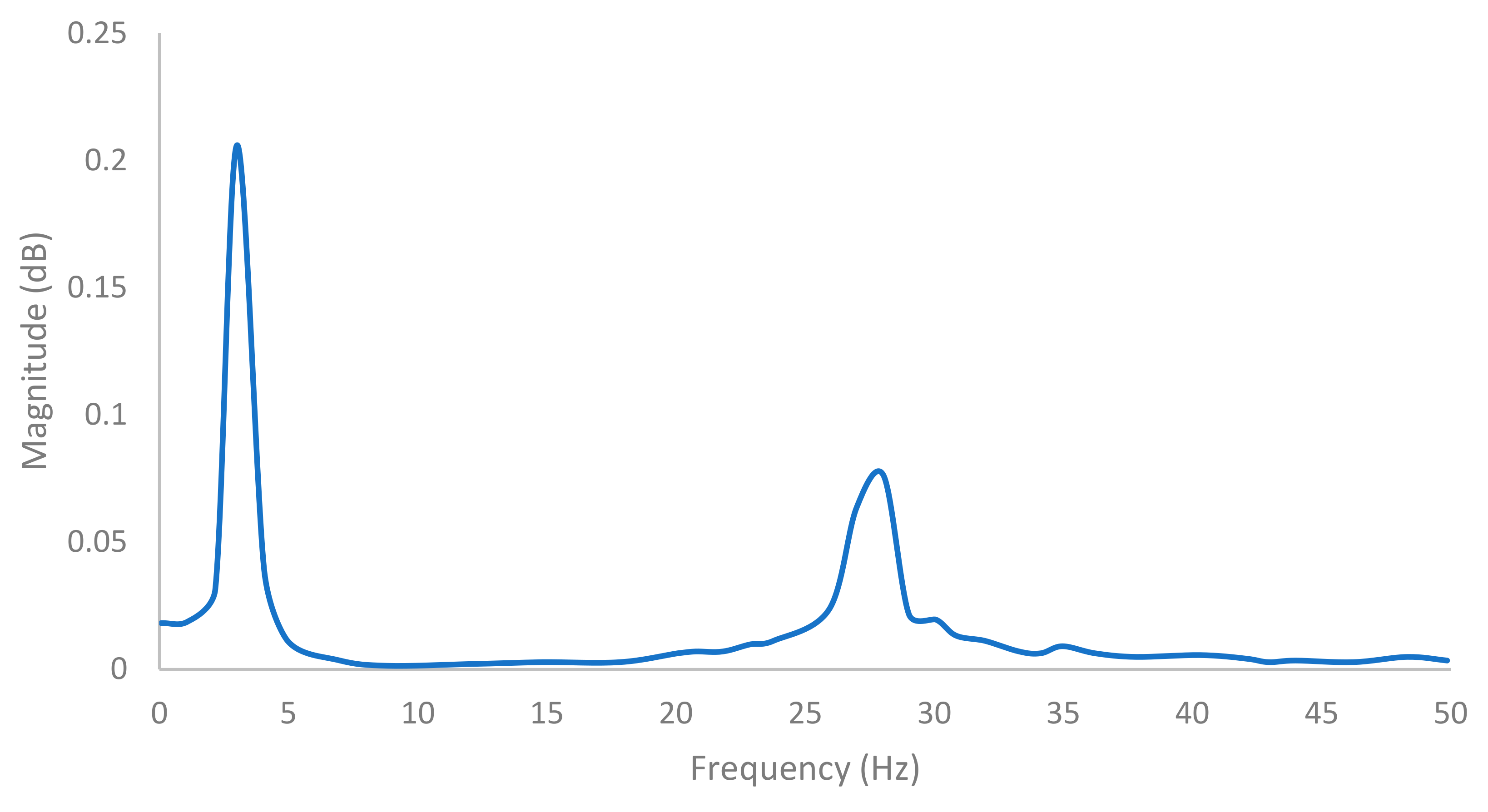
Figure 4.
Fast Fourier transform of the bridge’s vertical acceleration.
Figure 4.
Fast Fourier transform of the bridge’s vertical acceleration.
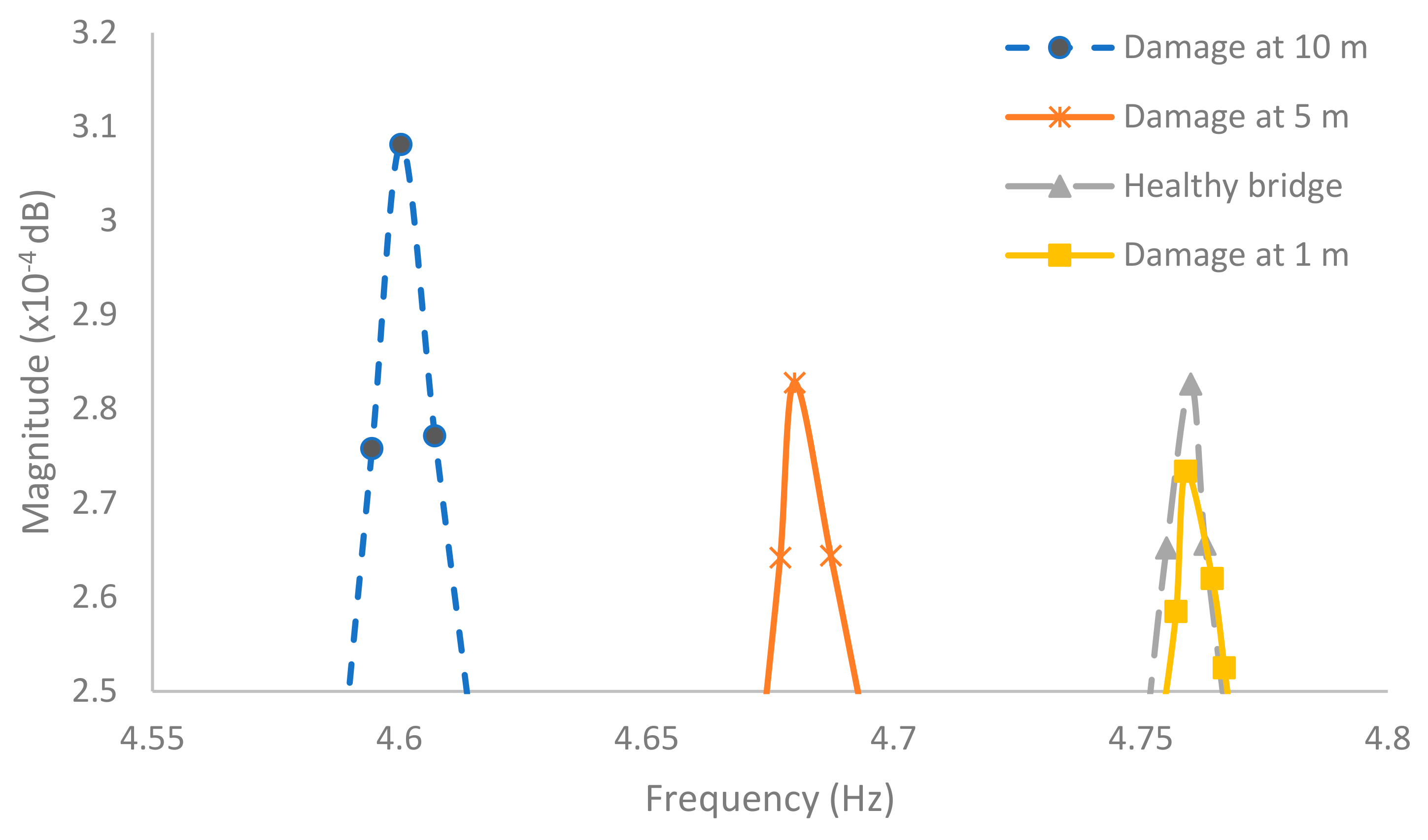
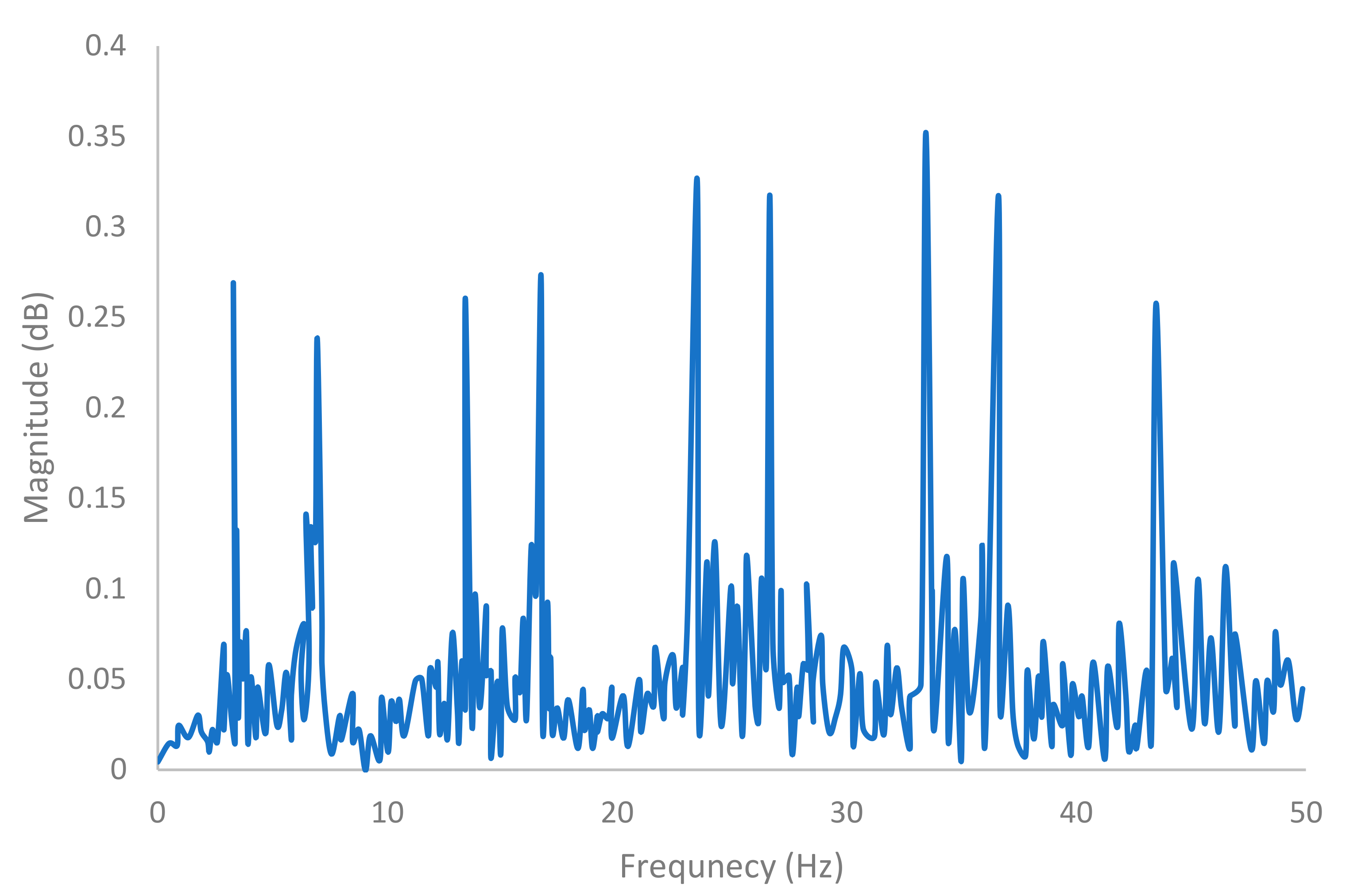
Figure 5.
Fast Fourier transform results in different damage locations.
Figure 5.
Fast Fourier transform results in different damage locations.
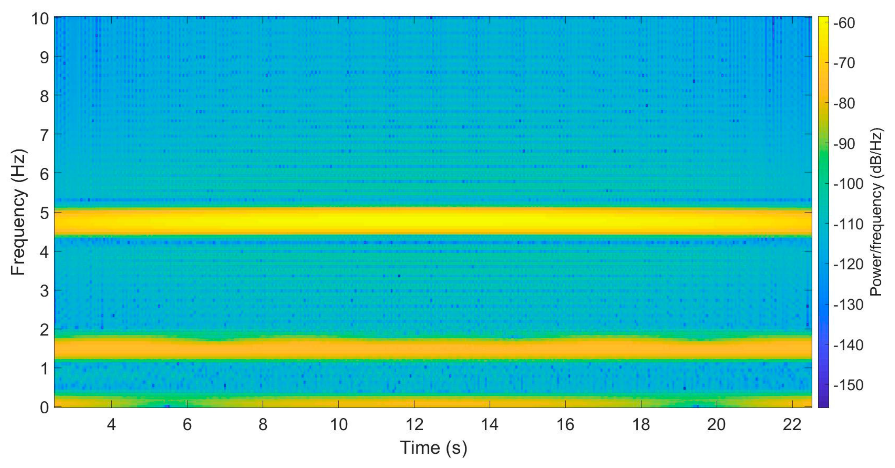
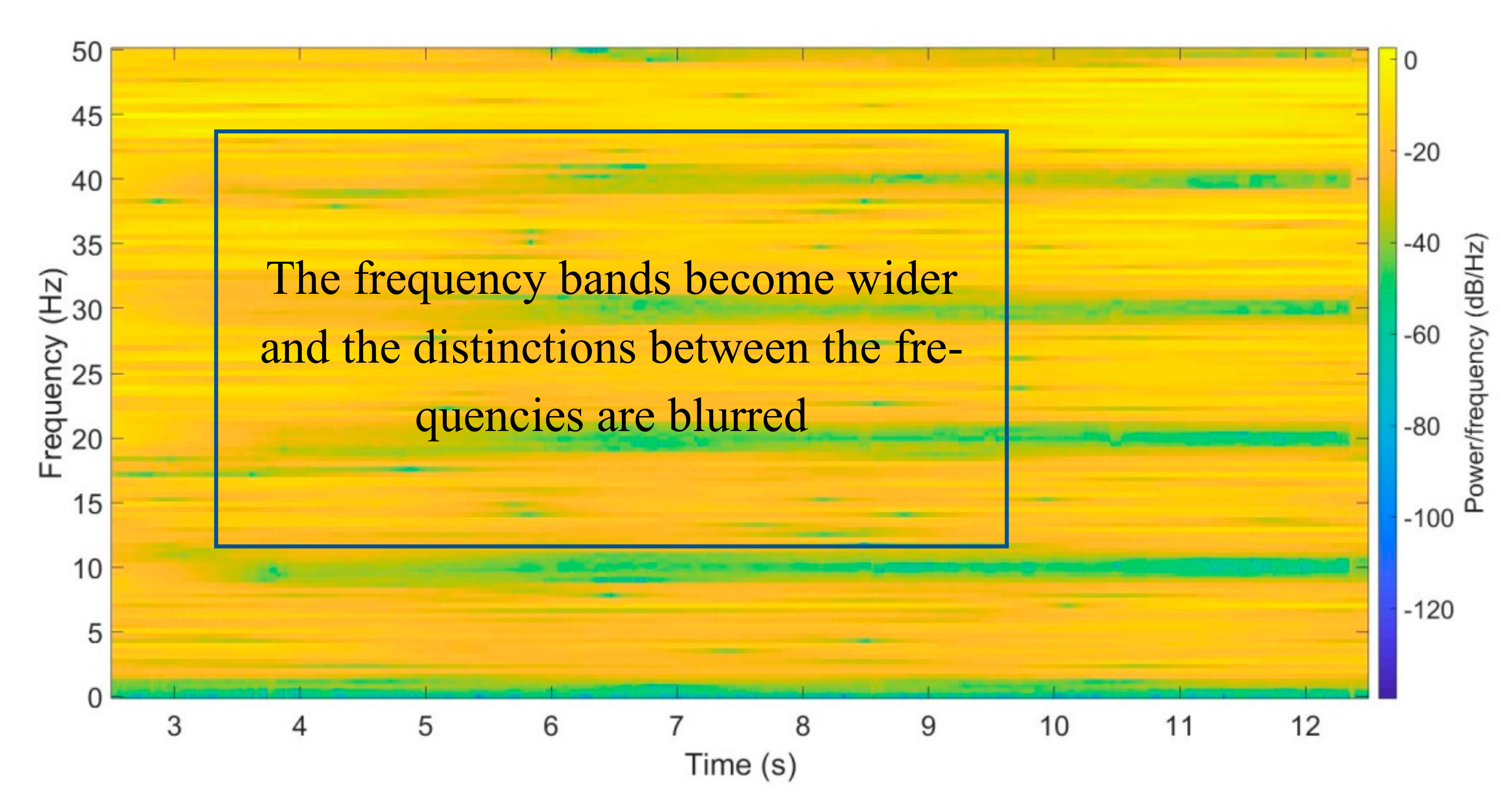
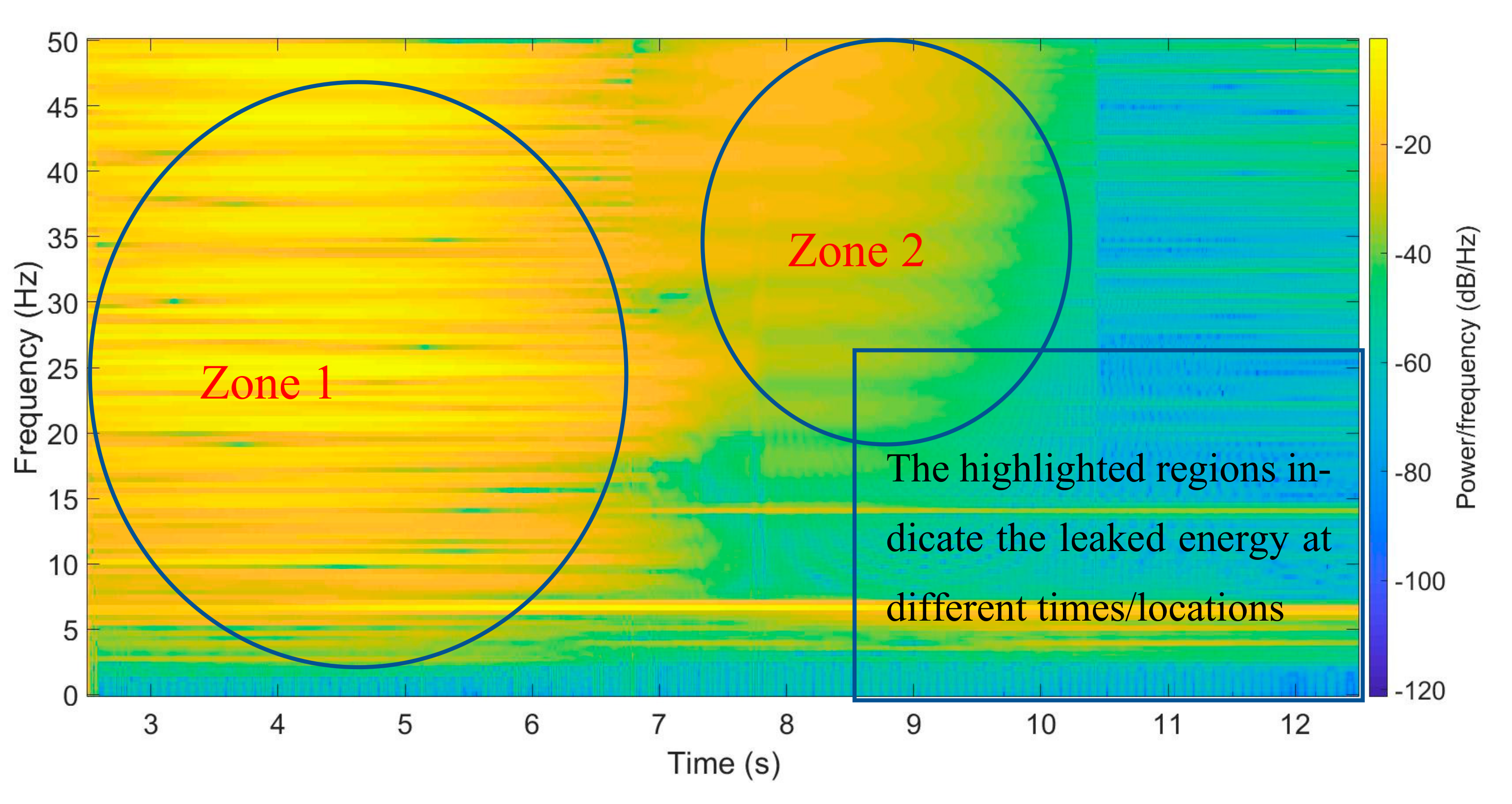
Figure 6.
Short-time Fourier transformation of the healthy bridge accelerations with window size 100.
Figure 6.
Short-time Fourier transformation of the healthy bridge accelerations with window size 100.
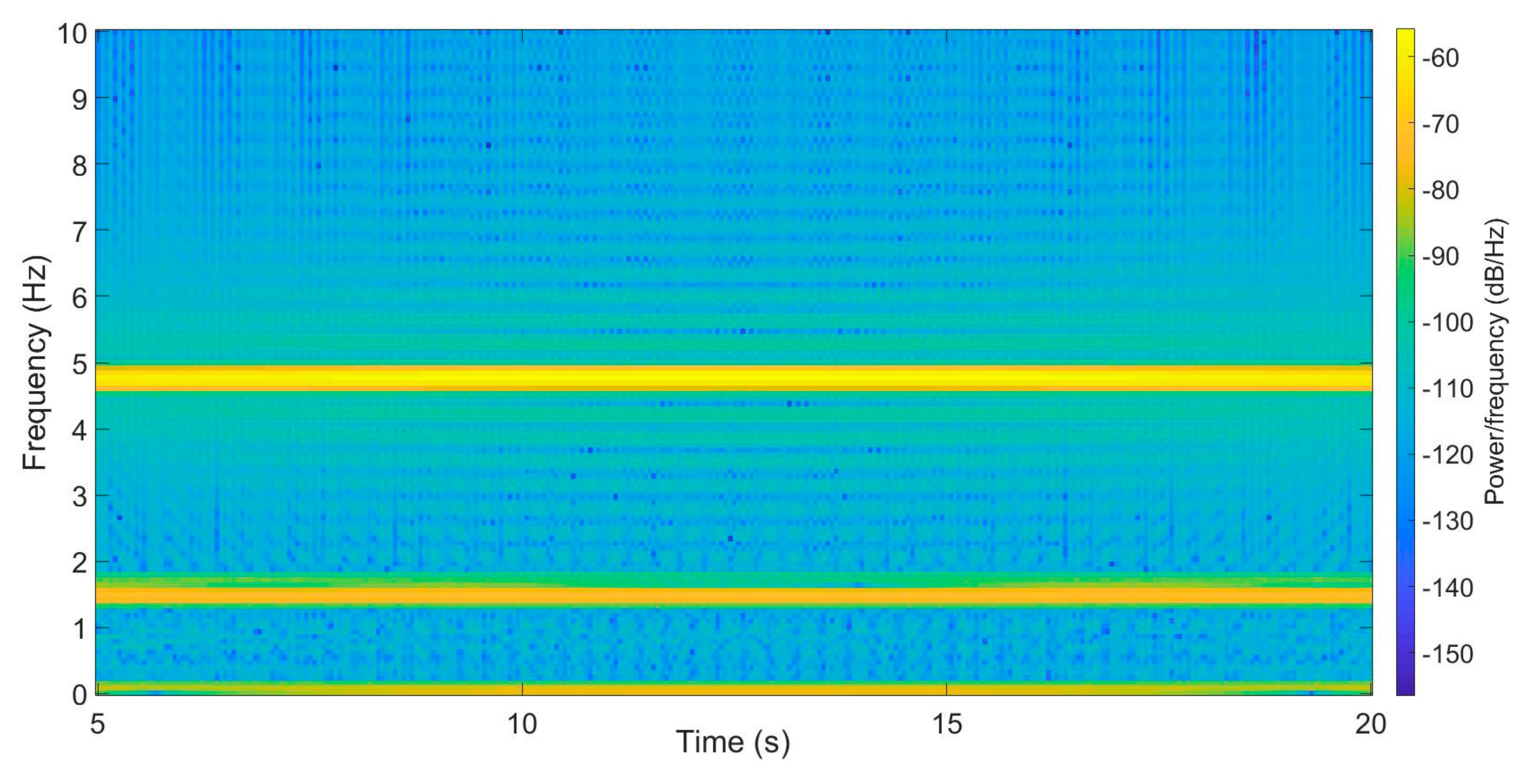
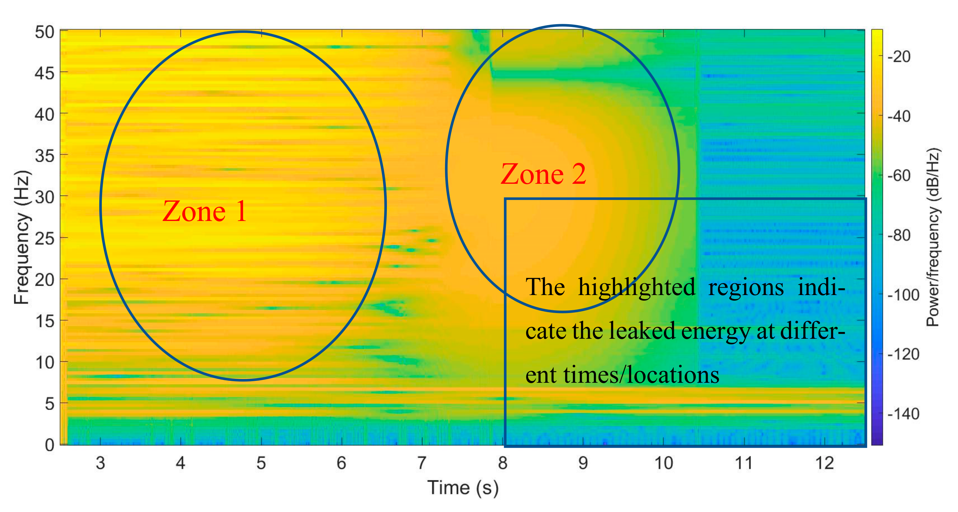
Figure 7.
Short-time Fourier transformation of the healthy bridge accelerations with window size 200.
Figure 7.
Short-time Fourier transformation of the healthy bridge accelerations with window size 200.
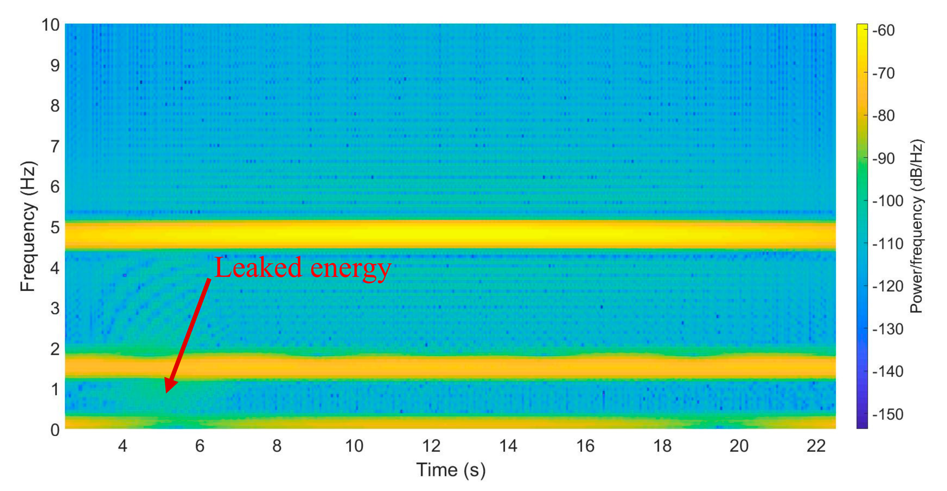
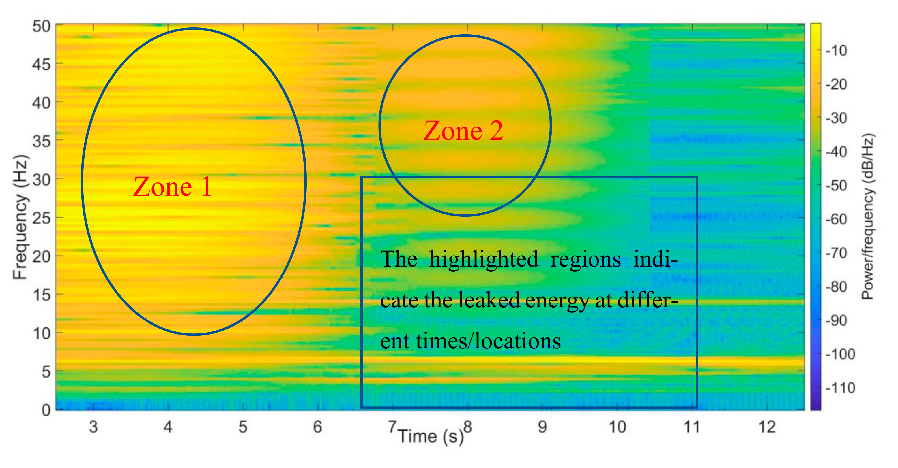
Figure 8.
Short-time Fourier transformation of the bridge accelerations with damage at 5 m location.
Figure 8.
Short-time Fourier transformation of the bridge accelerations with damage at 5 m location.
Figure 9.
Comparison of STFT results of bridge accelerations with different damage levels.
Figure 9.
Comparison of STFT results of bridge accelerations with different damage levels.
Figure 10.
Comparison of STFT results of bridge accelerations with multiple damages.
Figure 10.
Comparison of STFT results of bridge accelerations with multiple damages.
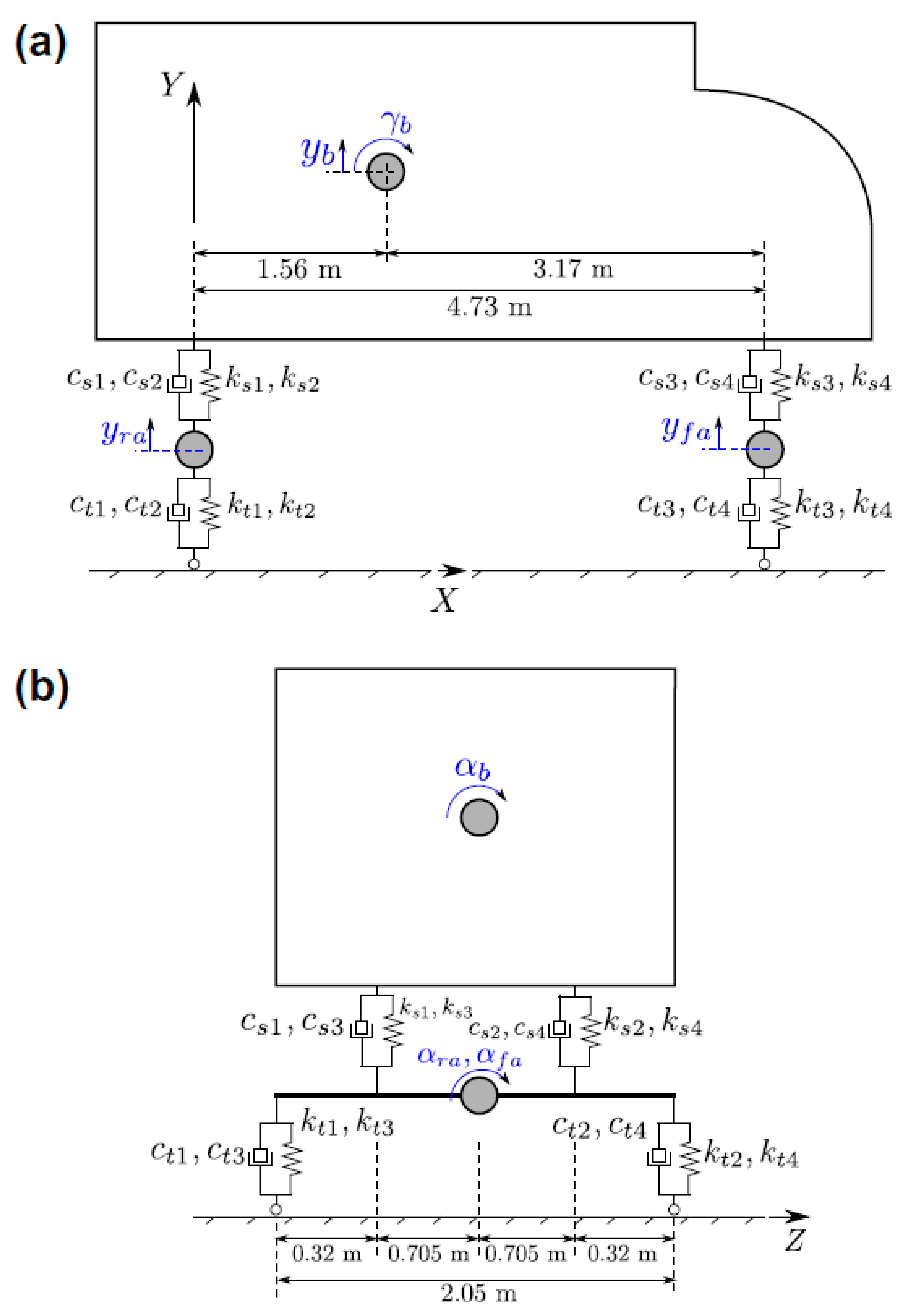
Figure 11.
Truck model: (a) side view, (b) rear view.
Figure 11.
Truck model: (a) side view, (b) rear view.
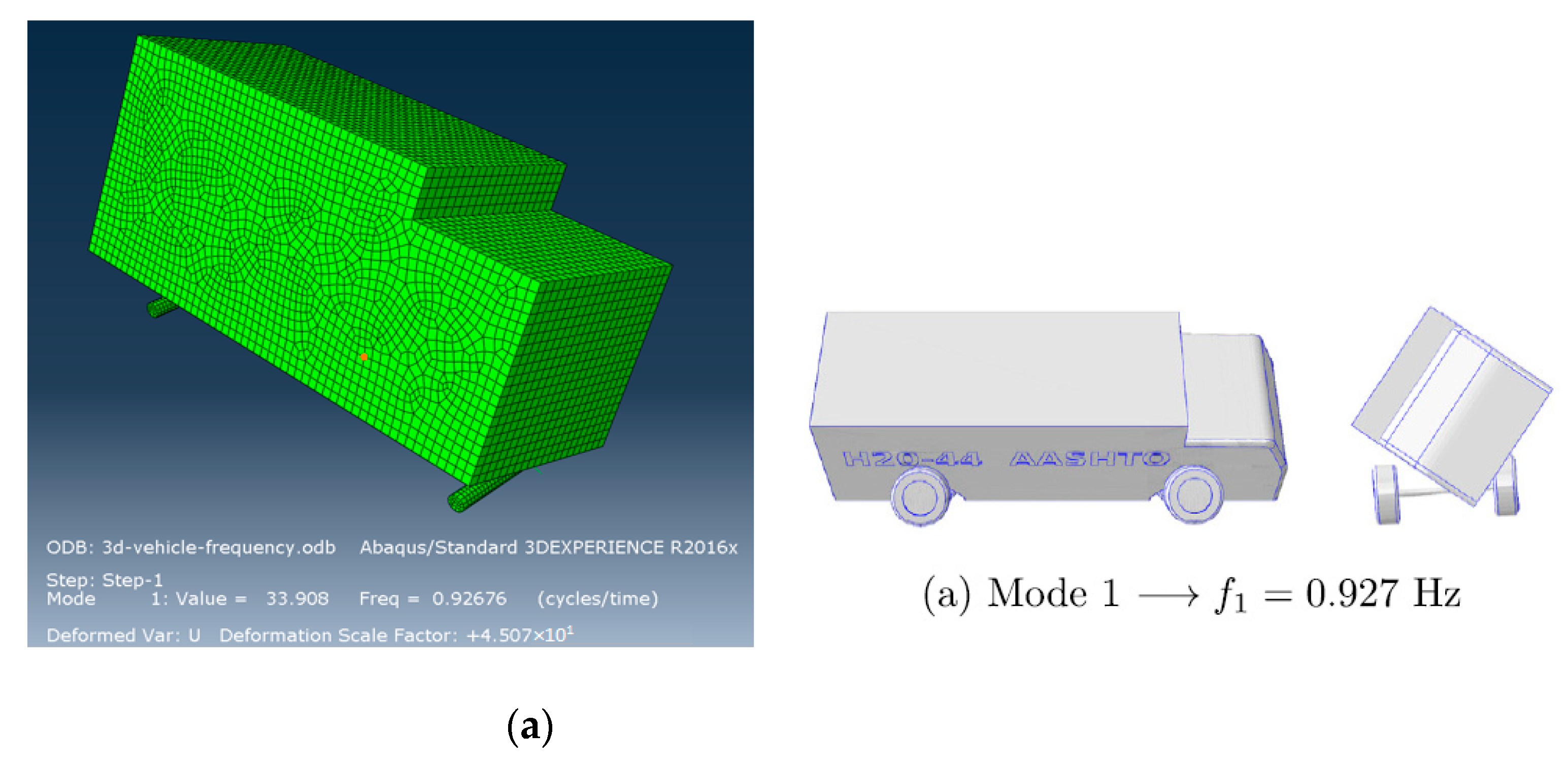
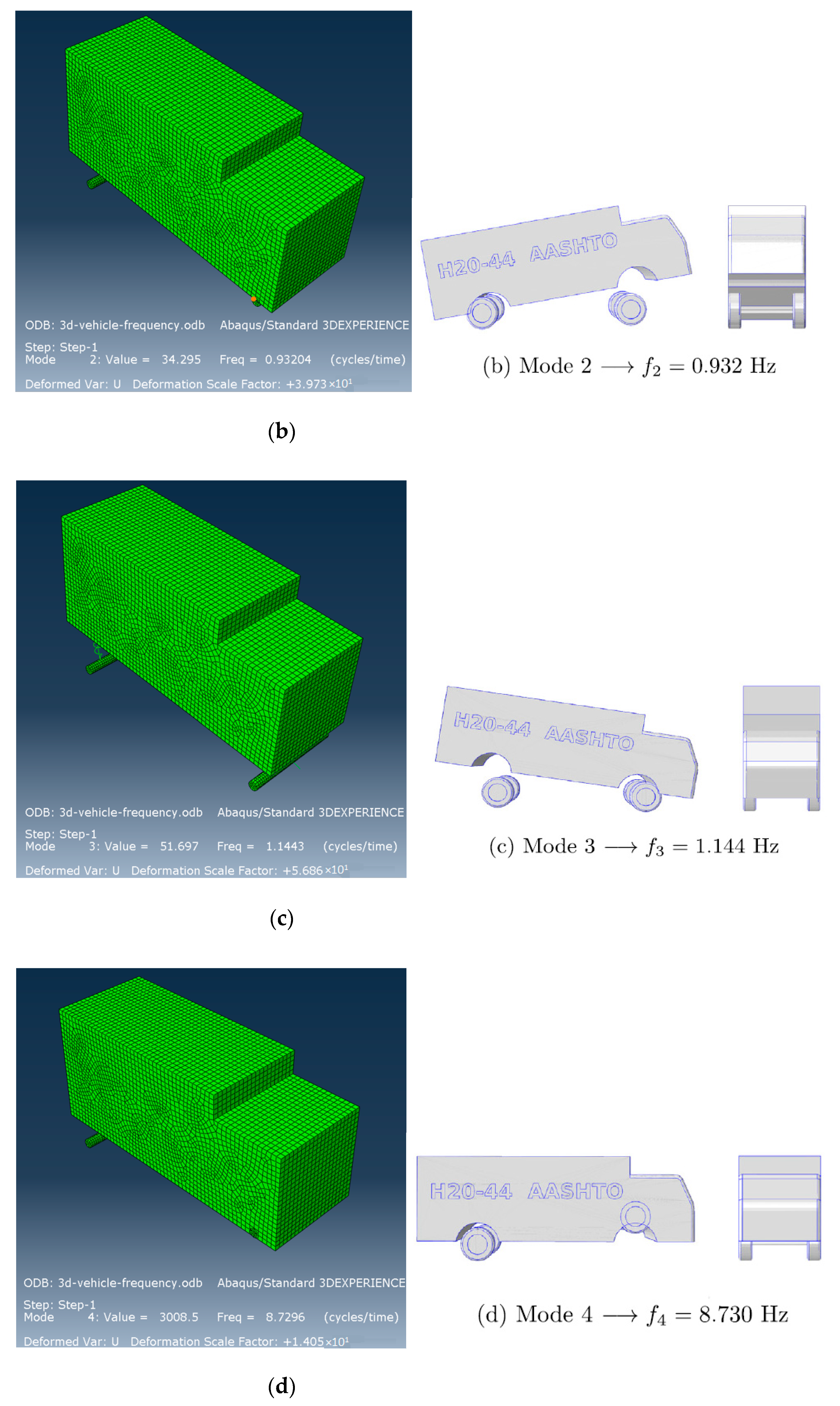
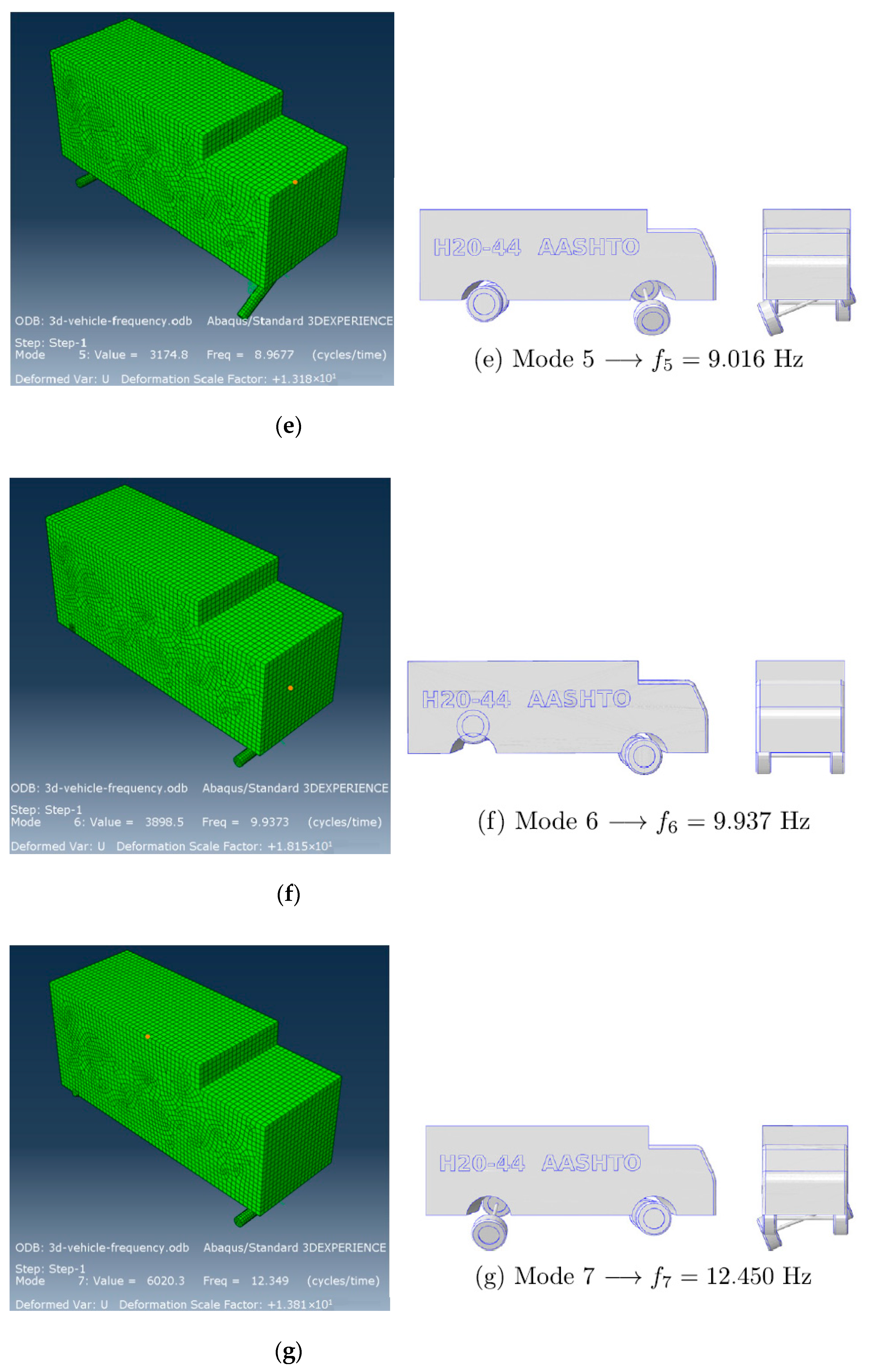
Figure 12.
Comparison of the model vehicle frequencies with the literature results. (a) Model 1, (b) Model 2, (c) Model 3, (d) Model 4, (e) Model 5, (f) Model 6, and (g) Model 7.
Figure 12.
Comparison of the model vehicle frequencies with the literature results. (a) Model 1, (b) Model 2, (c) Model 3, (d) Model 4, (e) Model 5, (f) Model 6, and (g) Model 7.
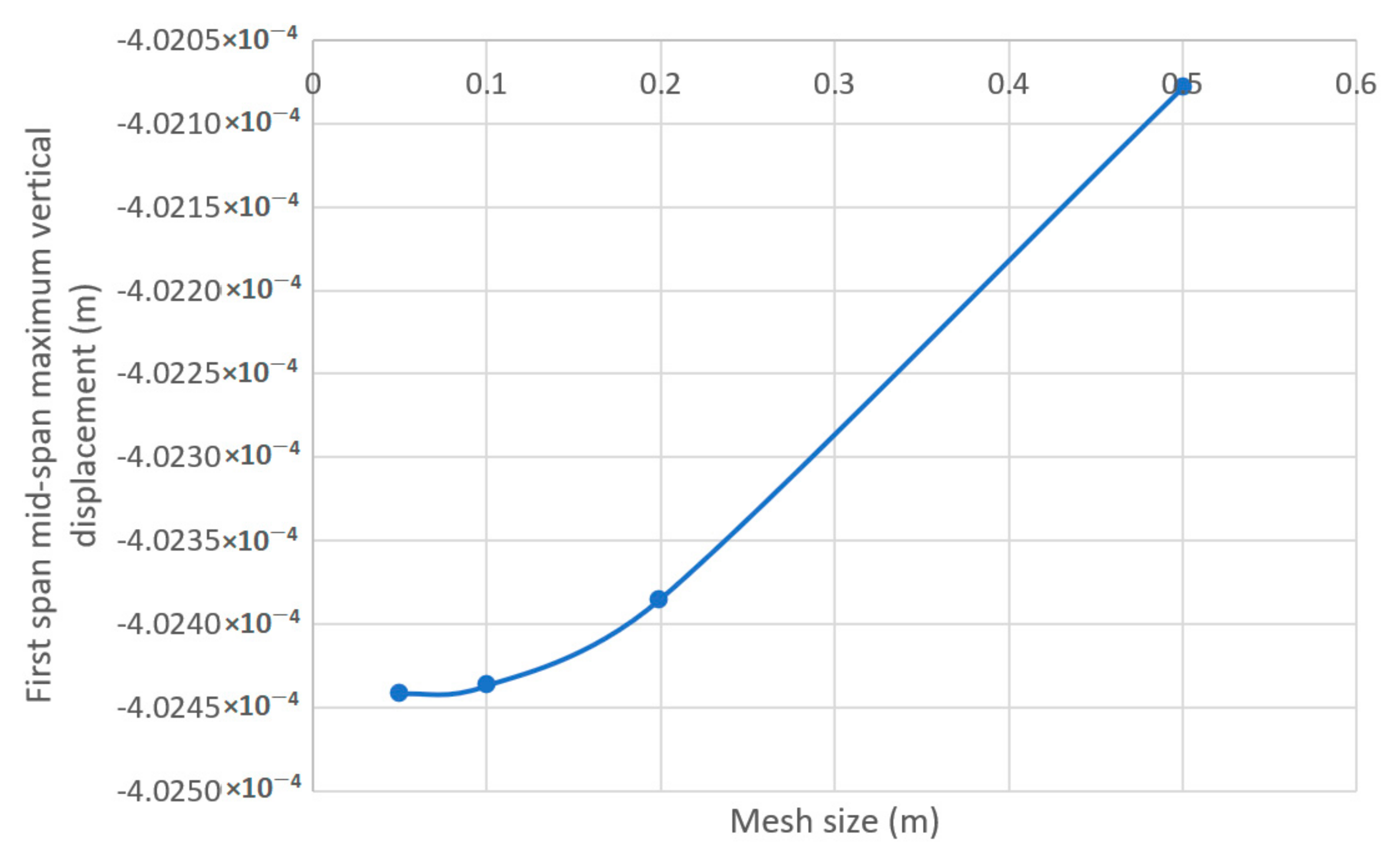
Figure 13.
Mesh sensitivity plot for the three-span bridge.
Figure 13.
Mesh sensitivity plot for the three-span bridge.
Figure 14.
The mid-span displacement time history of the first span when the truck passes at 32.5 m/s.
Figure 14.
The mid-span displacement time history of the first span when the truck passes at 32.5 m/s.
Figure 15.
Identified frequencies using the front tire acceleration time history.
Figure 15.
Identified frequencies using the front tire acceleration time history.
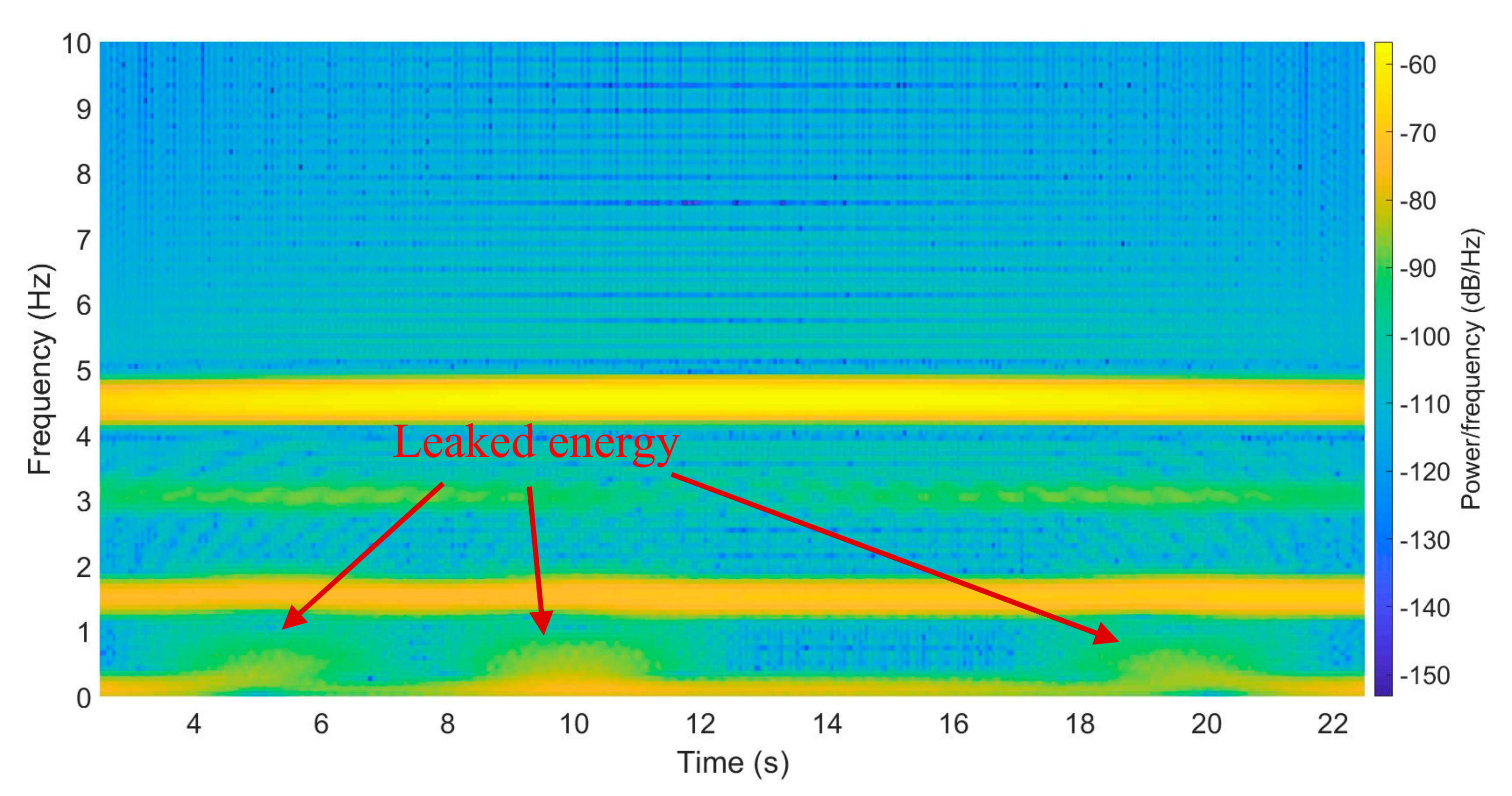
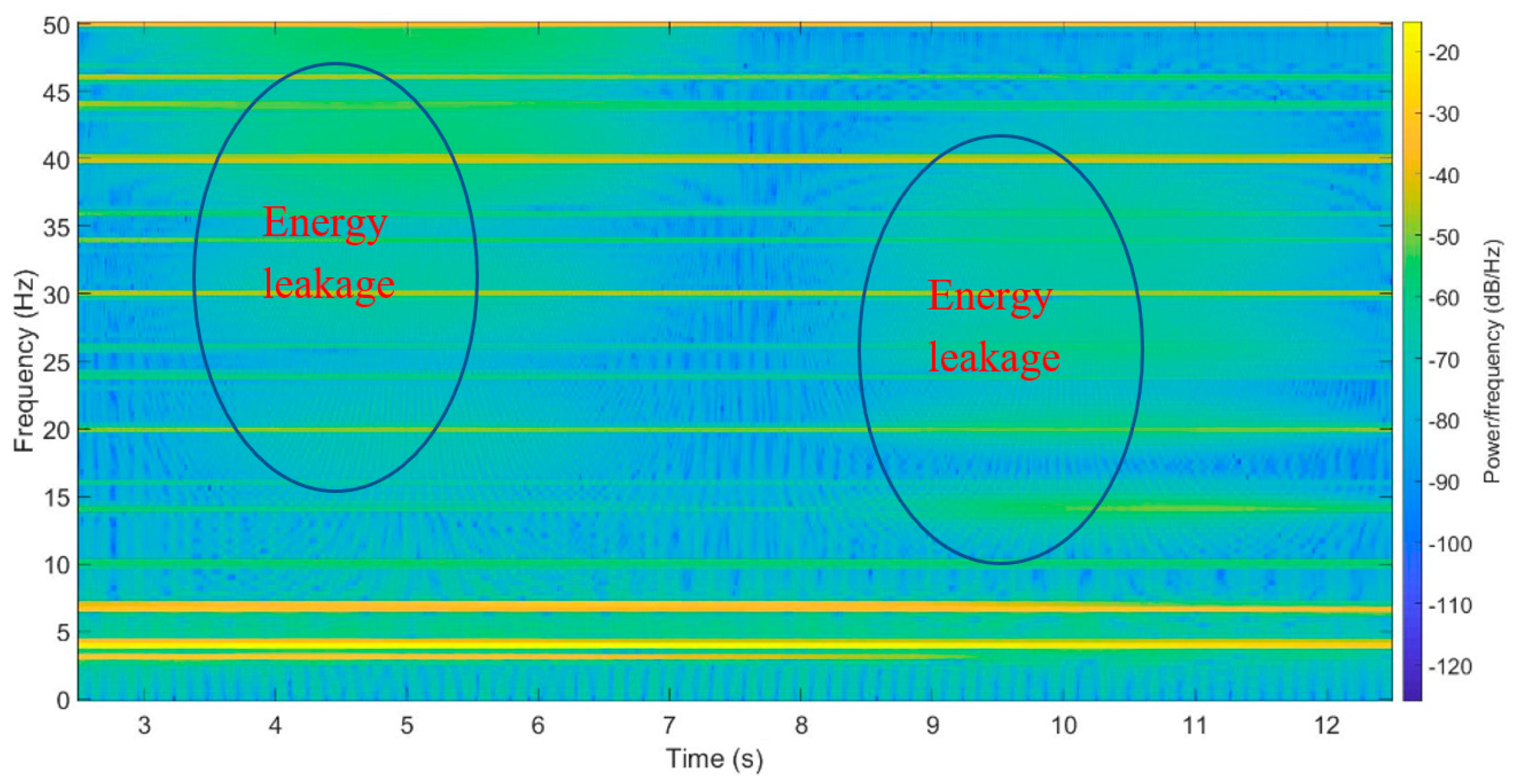
Figure 16.
STFT result of the bridge deck with a 10 cm damage at 5 m through the drive-by front tire acceleration time history (Energy leaked zones).
Figure 16.
STFT result of the bridge deck with a 10 cm damage at 5 m through the drive-by front tire acceleration time history (Energy leaked zones).
Figure 17.
STFT energy results for different damage levels.
Figure 17.
STFT energy results for different damage levels.
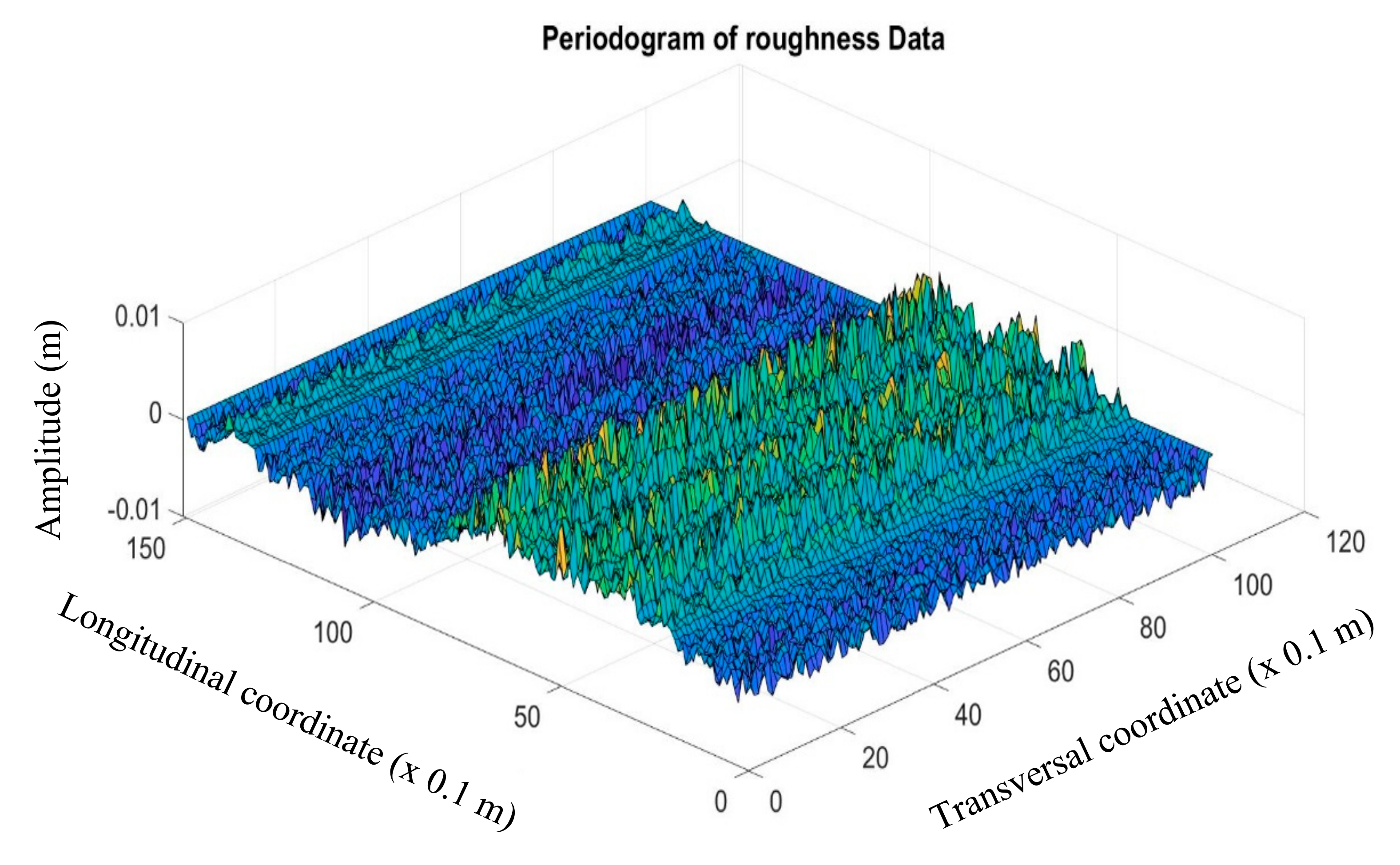
Figure 18.
Class B road roughness generated.
Figure 18.
Class B road roughness generated.
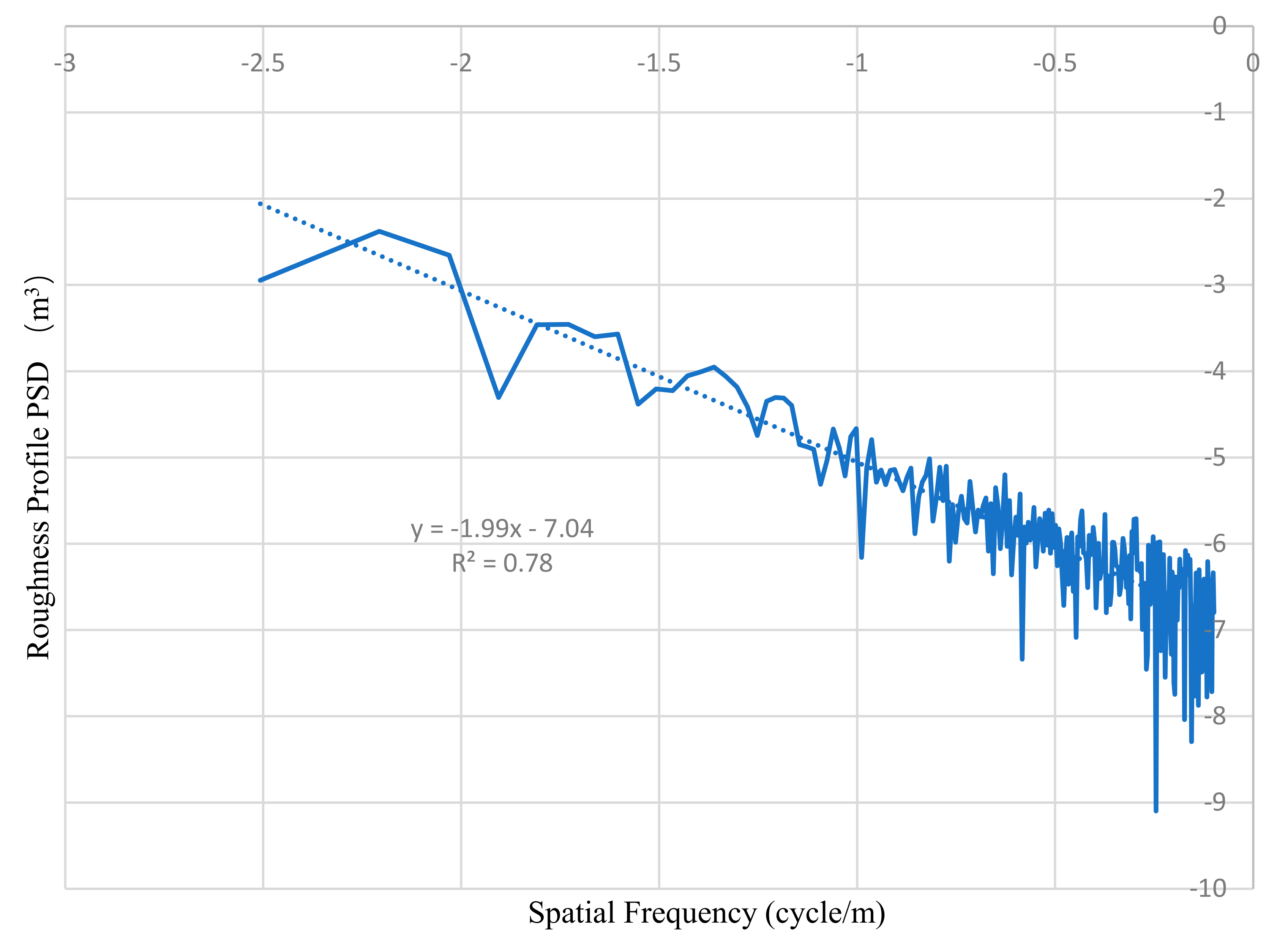
Figure 19.
Roughness profile PSDs versus spatial frequencies.
Figure 19.
Roughness profile PSDs versus spatial frequencies.
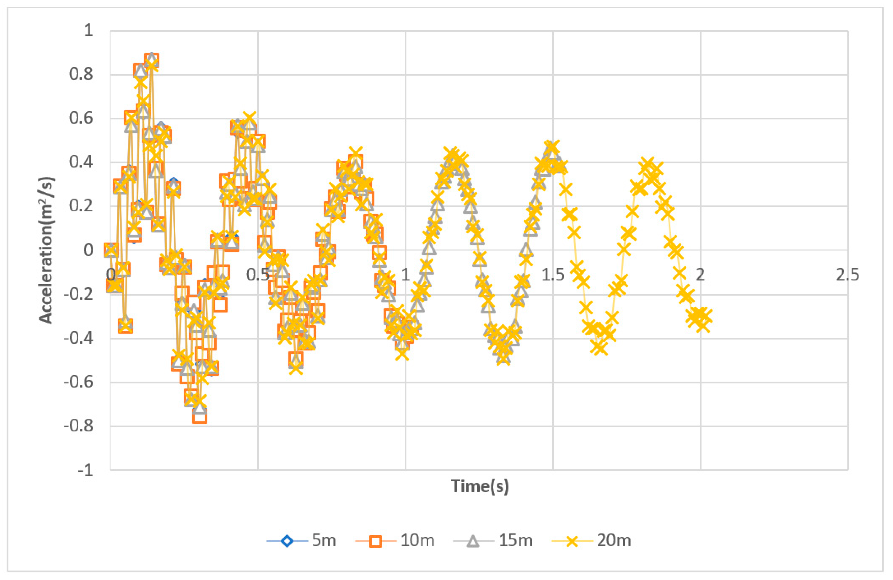
Figure 20.
Right front axle acceleration history when approaching the bridge at 10 m/s.
Figure 20.
Right front axle acceleration history when approaching the bridge at 10 m/s.
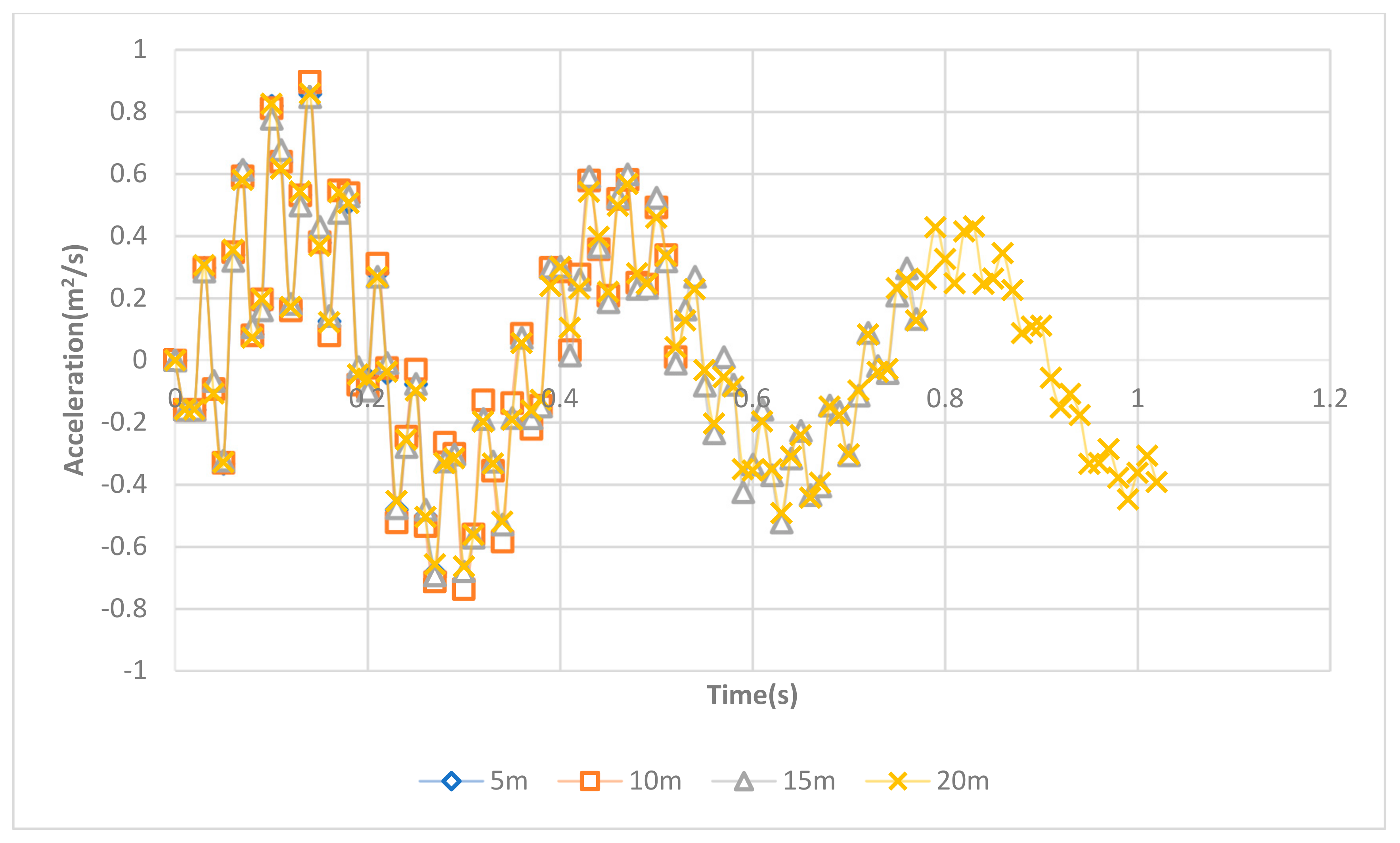
Figure 21.
Right front axle acceleration history when approaching the bridge at 20 m/s.
Figure 21.
Right front axle acceleration history when approaching the bridge at 20 m/s.
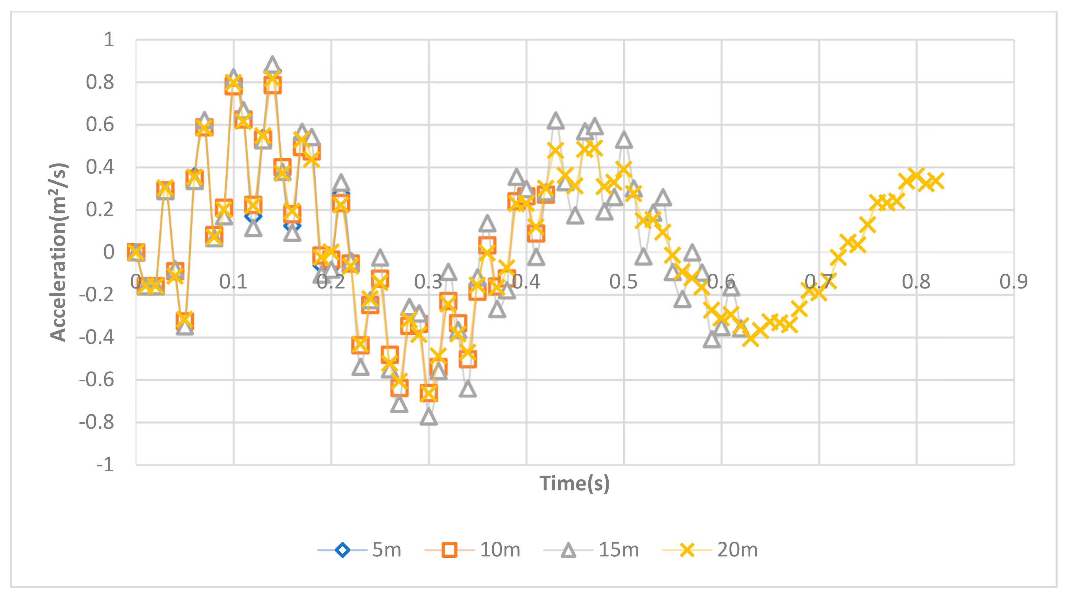
Figure 22.
Right front axle acceleration history when approaching the bridge at 25 m/s.
Figure 22.
Right front axle acceleration history when approaching the bridge at 25 m/s.
Figure 23.
Right front axle acceleration history when approaching the bridge at 30 m/s.
Figure 23.
Right front axle acceleration history when approaching the bridge at 30 m/s.
Figure 24.
FFT results of the vehicle acceleration responses when driving from a 20 m offset distance with a speed of 10 m/s.
Figure 24.
FFT results of the vehicle acceleration responses when driving from a 20 m offset distance with a speed of 10 m/s.
Figure 25.
FFT of right rear axle acceleration history of the VBI model on the bridge with the generated road roughness.
Figure 25.
FFT of right rear axle acceleration history of the VBI model on the bridge with the generated road roughness.
Figure 26.
STFT results of right rear axle acceleration history of the vehicle on undamaged bridges with the given roughness.
Figure 26.
STFT results of right rear axle acceleration history of the vehicle on undamaged bridges with the given roughness.
Figure 27.
STFT results of vehicle’s right rear axle acceleration difference between the 40% damage case and the healthy bridge.
Figure 27.
STFT results of vehicle’s right rear axle acceleration difference between the 40% damage case and the healthy bridge.
Figure 28.
STFT results of vehicle’s right rear axle acceleration difference between the 60% damage case and the healthy bridge.
Figure 28.
STFT results of vehicle’s right rear axle acceleration difference between the 60% damage case and the healthy bridge.
Figure 29.
STFT results of vehicle’s right rear axle acceleration difference between the 80% damage case and the healthy bridge.
Figure 29.
STFT results of vehicle’s right rear axle acceleration difference between the 80% damage case and the healthy bridge.
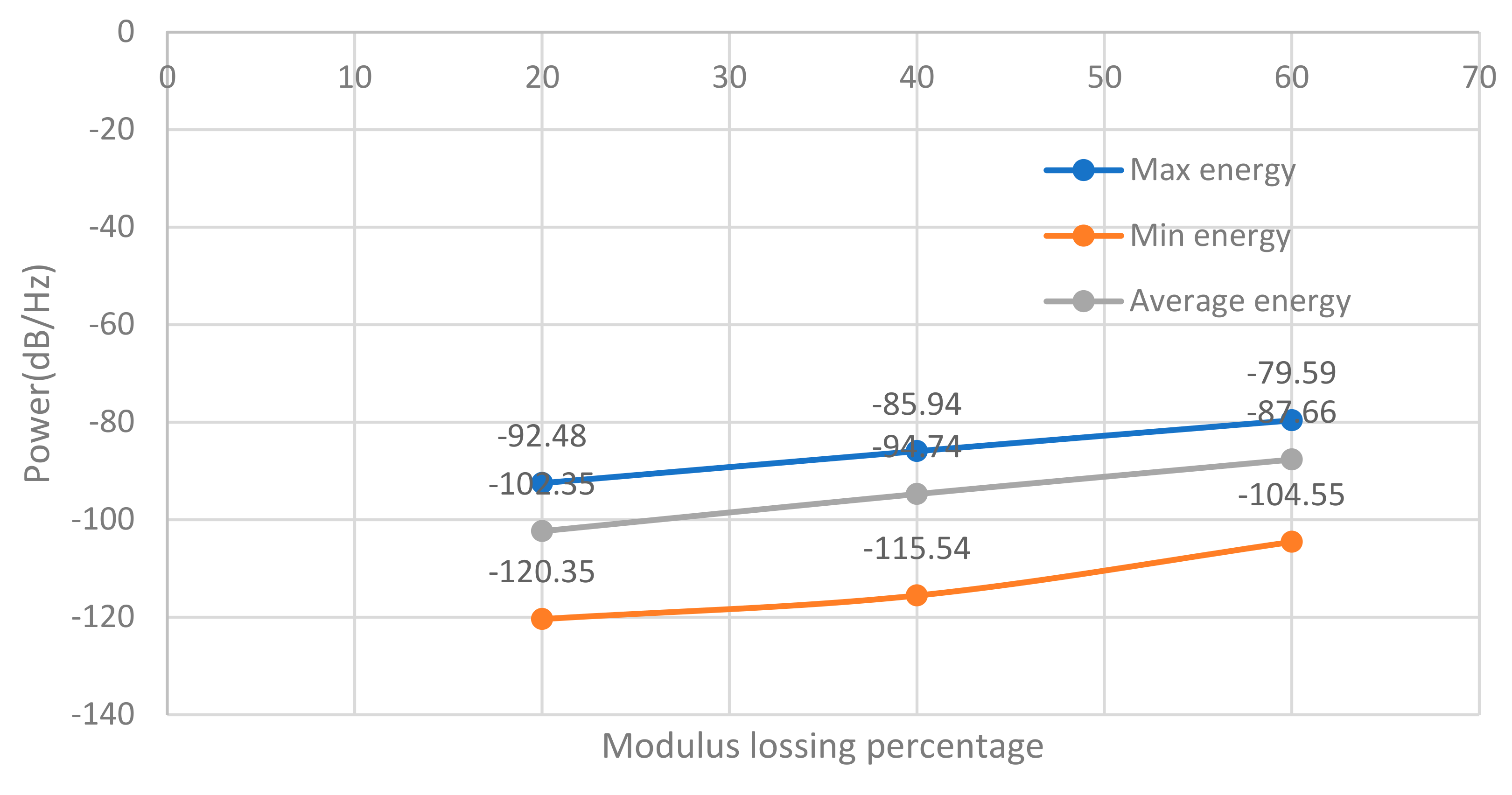
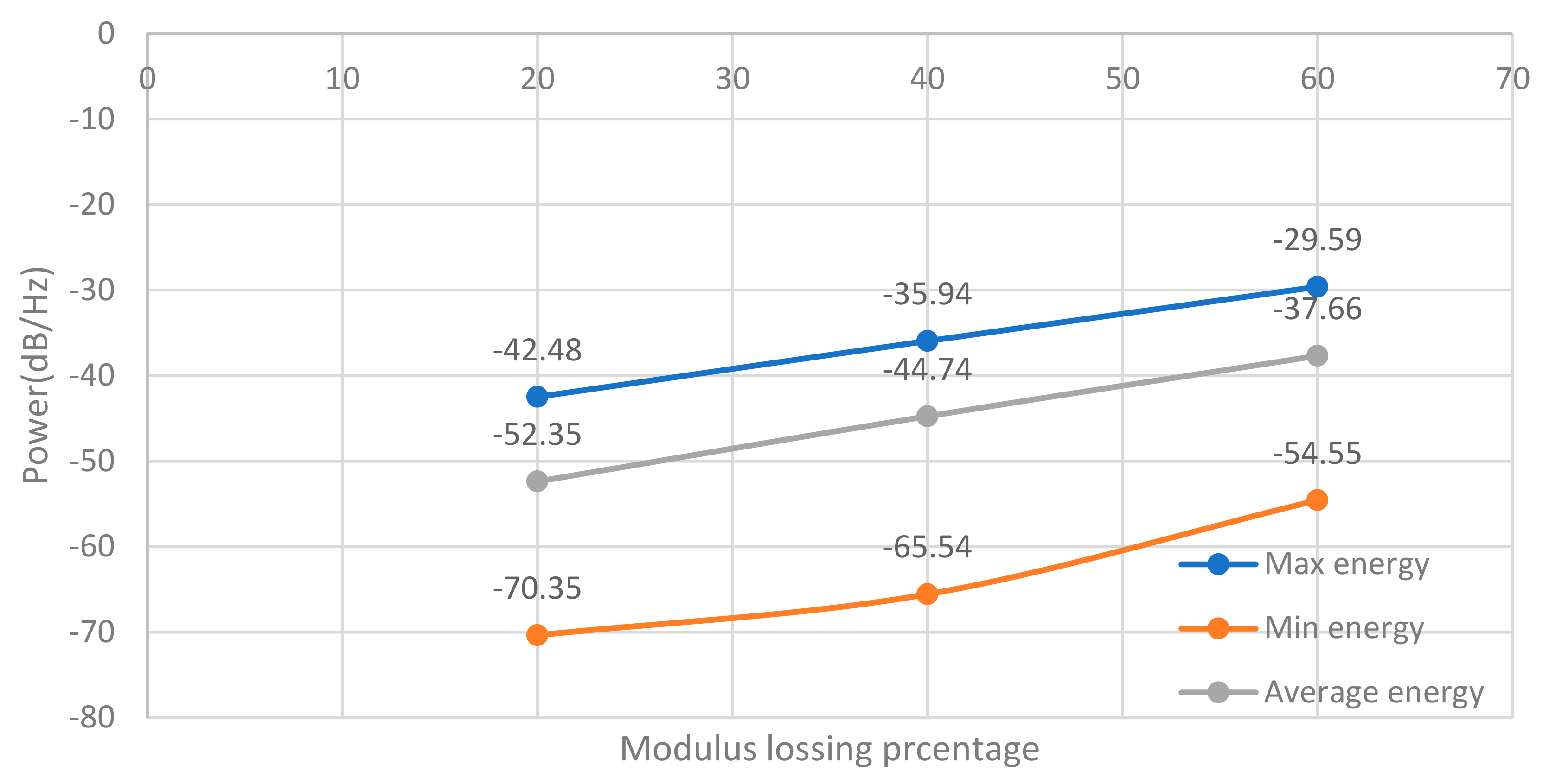
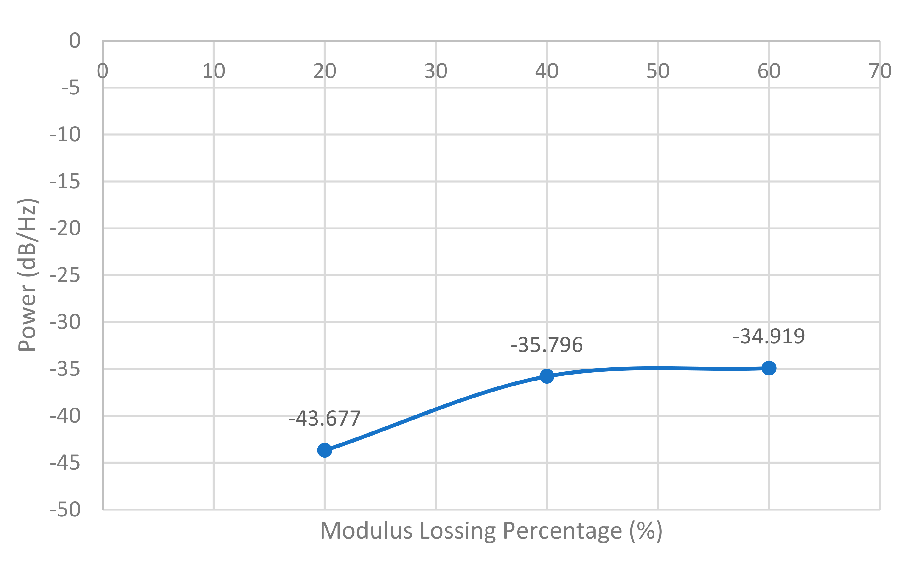
Figure 30.
Average PSD energy over the damaged area (7.5 m to 7.6 m).
Figure 30.
Average PSD energy over the damaged area (7.5 m to 7.6 m).
Table 1.
List of damaged model conditions.
Table 1.
List of damaged model conditions.
| Model # | Damage Location | Young’s Modulus | Damage Size |
|---|
| 1, 2, 3 | 1 m | 20% loss | 0.1 m, 0.5 m, 1 m |
| 4, 5, 6 | 5 m | 20% loss | 0.1 m, 0.5 m, 1 m |
| 7, 8, 9 | 10 m | 20% loss | 0.1 m, 0.5 m, 1 m |
| 10, 11, 12 | 12.5 m | 20% loss | 0.1 m |
| 40% loss |
| 60% loss |
Table 2.
Comparison of Short-Time Fourier Transform (STFT) results of different damage locations on the bridge.
Table 2.
Comparison of Short-Time Fourier Transform (STFT) results of different damage locations on the bridge.
| Cases | Real Mid Location(m) | Identified Results |
|---|
| Start Location (m) | End Location (m) | Mid Location (m) | Ave Energy (dB/Hz) |
|---|
| 1 m damage at 1 m location | 1.5 | 2.5 | 3.45 | 2.975 | −101.06 |
| 1 m damage at 5 m location | 5.5 | 3.25 | 7.85 | 5.55 | −97.234 |
| 1 m damage at 10 m location | 10.5 | 8.05 | 12.95 | 10.5 | −95.321 |
Table 3.
Comparison of STFT results of bridges with different damage sizes.
Table 3.
Comparison of STFT results of bridges with different damage sizes.
| Cases | Real Mid Location(m) | Real Damaged Length(m) | Identified Results |
|---|
| Start Location(m) | End Location(m) | Mid Location(m) | Damaged Length (m) | Ave Energy (dB/Hz) |
|---|
| 1 m damage at 10 m location | 10.5 | 1 | 8.05 | 12.95 | 10.5 | 4.9 | −95.321 |
| 0.5 m damage at 5 m location | 10.25 | 0.5 | 8.05 | 12.4 | 10.225 | 4.35 | −93.278 |
| 0.1 m damage at 10 m location | 10.05 | 0.1 | 8.5 | 11.6 | 10.05 | 3.1 | −101.667 |
Table 4.
The mechanical parameters of the vehicle.
Table 4.
The mechanical parameters of the vehicle.
| Element | Notation | Value |
|---|
| Stiffness(N/m) |
| Rear wheels | Kt1, kt2 | 1.57 × 10⁶ |
| Front wheels | Kt3, kt4 | 7.85 × 10⁵ |
| Rear suspensions | Ks1, ks2 | 3.73 × 10⁵ |
| Front suspension | Ks3, ks4 | 1.16 × 10⁵ |
| Dampings (N*s/m) |
| Rear wheels | Ct1, Ct2 | 200 |
| Front wheels | Ct3, Ct4 | 100 |
| Rear suspensions | Cs1, Cs2 | 35,000 |
| Front suspension | Cs3, Cs4 | 25,000 |
| Masses (Kg) |
| Rear axle | mra | 1000 |
| Front axle | mfa | 600 |
| Body | mb | 17,000 |
| Rotatory Inertias (kg*m2) |
| Rear axle (roll) | Iα,ra | 600 |
| Front axle (roll) | Iα,fa | 550 |
| Body (roll) | Iα,b | 13,000 |
| Body (pitch) | Iγ,b | 90,000 |
Table 5.
Identified bridge frequencies through the front tire acceleration time history.
Table 5.
Identified bridge frequencies through the front tire acceleration time history.
| | Reference Bridge Frequencies (Hz) |
|---|
| 4.83 | 6.21 | 9.13 | 16.23 | 17.24 | 18.57 | 18.91 | 20.94 |
|---|
| FFT Results | 4.65 | 6.65 | 10.00 | 16.65 | | 18.45 | | 20.00 |
Table 6.
Properties of the simulated short bridge.
Table 6.
Properties of the simulated short bridge.
| Length | 15 m | Young′s Modulus | 3E10 N/m2 |
|---|
| Width | 10 m | Poisson’s modulus | 0.2 |
| Thickness | 1 m | Density | 2500 Kg/m3 |
| Damping | 2% | | |
Table 7.
Comparison of the predicted and real damage locations.
Table 7.
Comparison of the predicted and real damage locations.
| Cases | Real Mid Location(m) | Identified Results |
|---|
| Start Location (m) | End Location (m) | Mid Location (m) | Error (m) | Aver. Energy (dB/Hz) |
|---|
| 0.1 m damage at 5 m location | 5.05 | 4.81 | 5.3 | 5.05 | 0 | −88.06 |
| 0.1 m damage at 7.5 m location | 7.55 | 7.21 | 7.85 | 7.53 | 0.02 | −87.73 |
| 0.1 m damage at 10 m location | 10.05 | 9.05 | 10.95 | 10.0 | 0.05 | −106.87 |
Table 8.
Road roughness classification.
Table 8.
Road roughness classification.
| Road Class | G(n0) (m3) |
|---|
| A (very good) | 1.600 × 10⁻⁵ |
| B (good) | 6.400 × 10⁻⁵ |
| C (medium) | 2.560 × 10⁻⁴ |
| D (poor) | 1.024 × 10⁻³ |
| E (very poor) | 4.096 × 10⁻³ |
Table 9.
Acceleration amplitude for the 3 Hz component in the vehicle’s vibration.
Table 9.
Acceleration amplitude for the 3 Hz component in the vehicle’s vibration.
| | Driving Distance |
|---|
| 5 m | 10 m | 15 m | 20 m |
|---|
| Driving Speed | 10 m/s | 0.393 | 0.384 | 0.423 | 0.312 |
| 20 m/s | 0.491 | 0.412 | 0.373 | 0.377 |
| 25 m/s | 0.511 | 0.498 | 0.384 | 0.341 |
| 30 m/s | 0.518 | 0.508 | 0.386 | 0.352 |
Table 10.
Acceleration amplitude for the 28 Hz component in the vehicle’s vibration.
Table 10.
Acceleration amplitude for the 28 Hz component in the vehicle’s vibration.
| | Driving Distance |
|---|
| 5 m | 10 m | 15 m | 20 m |
|---|
| Driving speed | 10 m/s | 0.14 | 0.036 | 0.003 | 0.021 |
| 20 m/s | 0.202 | 0.124 | 0.103 | 0.07 |
| 25 m/s | 0.285 | 0.211 | 0.121 | 0.019 |
| 30 m/s | 0.334 | 0.266 | 0.123 | 0.116 |
Table 11.
Comparison of identified bridge frequencies and the theoretical bridge frequencies (Hz).
Table 11.
Comparison of identified bridge frequencies and the theoretical bridge frequencies (Hz).
| | Bridge Frequencies |
|---|
| Theoretical bridge frequency | | 7 | | 15.4 | | 28 | | 38.6 | |
| Identified frequency | 3.4 | 6.94 | 13.4 | 16.6 | 23.4 | 26.6 | 33.4 | 36.6 | 43.4 |


