Abstract
Texture plays an important role in computer vision in expressing the characteristics of a surface. Texture complexity evaluation is important for relying not only on the mathematical properties of the digital image, but also on human perception. Human subjective perception verbally expressed is relative in time, since it can be influenced by a variety of internal or external factors, such as: Mood, tiredness, stress, noise surroundings, and so on, while closely capturing the thought processes would be more straightforward to human reasoning and perception. With the long-term goal of designing more reliable measures of perception which relate to the internal human neural processes taking place when an image is perceived, we firstly performed an electroencephalography experiment with eight healthy participants during color textural perception of natural and fractal images followed by reasoning on their complexity degree, against single color reference images. Aiming at more practical applications for easy use, we tested this entire setting with a WiFi 6 channels electroencephalography (EEG) system. The EEG responses are investigated in the temporal, spectral and spatial domains in order to assess human texture complexity perception, in comparison with both textural types. As an objective reference, the properties of the color textural images are expressed by two common image complexity metrics: Color entropy and color fractal dimension. We observed in the temporal domain, higher Event Related Potentials (ERPs) for fractal image perception, followed by the natural and one color images perception. We report good discriminations between perceptions in the parietal area over time and differences in the temporal area regarding the frequency domain, having good classification performance.
1. Introduction
Visual perception is a complex process, enveloping various sub-processes. The visual information crosses through the optical system and along with light excites the retina’s photoreceptors. The resulting electrical information is transferred to the visual cortex, communicating with other areas of the brain in order to process the perceived information. At this step, the internal thought processes interpret the perceived information. However, the action of processing the external information perceived by the nervous system is not completely understood [1].
Texture analysis is of particular interest in various domains like computer vision, biomedical sciences, medical imaging, geographic information systems and many more [2], while fractal models are very popular for generating synthetic color textures. When referring to color image complexity, the notion is investigated in various domains which include surface analysis, artificial vision and human perception. The quest would be to express image complexity as accurately as possible, by taking into account different aspects, such as: The nature of the texture—being either natural or synthetic; the novelty—being familiar or novel to a human observer; its organization—recognizable structures or purely stochastic. In this matter, would be interesting to determine if differences would arise between natural and synthetic textures: Would they be differently perceived by humans? Would novelty and structural organization influence complexity perception? So far, the complexity of fractal color images is mathematically expressed by various measures [3,4,5], with the most common being the fractal dimension and entropy [3,6,7,8] or by metrics based on image segmentation [9]. An interesting approach for evaluating visual complexity, suitable for creative works such as paintings, uses an objective metric derived from neuroscience termed Artistic Complexity which looks into the average mutual information of different sub-parts of the images [10,11]. Other approaches for estimating image complexity rely on image compressing mechanisms which operate by removing as much information as possible [12,13,14], which however does not relate well to human perception since small visual elements are highly valuable to the human eye being discriminative between subtle degrees of complexity. Therefore, image complexity estimation seems insufficient without considering the human perception and interpretation, which can differ [15,16,17]. Image complexity perception, investigated so far, more in terms of human subjective descriptions [15,18], is viewed as being related to the objective characteristics of a texture which relate strongly with the subjective knowledge of the interviewees in study [19]. Though, human subjective assessment lacks generalization due to the increased variation in reporting between different individuals, being additionally influenced by internal factors determined by individuals’ mood or fatigue [20]. Therefore, the definition of color image complexity requires objective compensatory measures, such as the underlying processes of the neural activity itself.
In this sense, one technology that proved to be suitable for recording and interpreting the neural activity is electroencephalography (EEG), technique widely used in visual perception research which records the cortical electrical activity [21,22,23,24,25]. When studying perception, one may rely strictly on the analysis of the key features of the visual system, like studying the visual pathway, from the photoreceptors cell responses of visual objects towards the representation in the visual cortex, which does not express how the information is interpreted in the brain. The human perception process includes an internal threshold of detection at the cognitive level which helps in interpretation, reasoning and decision making on the degree of image complexity, which cannot be determined strictly within the visual processing stages. Studying other brain areas where the activity is transferred is more likely to provide sufficient relevant information on complexity perception. Whereas techniques such as PET and fMRI would better capture the functional interactions between different brain areas, they can not easily be used in practice. Targeting future practical applications, a simpler system, like one based on EEG would be beneficial, taking into account the compactness and the possibility to remotely scan the scalp and acquire neural signals [26]. Similarly to the analysis of visual perception as researched so far [25], or with the analysis of neural perception on complexity tasks, the neural responses on perception of complexity of images can be investigated with EEG. The brain responses elicited by an external stimulus, in an Oddball paradigm, where external stimuli are presented in form of a Target/Non-Target scenario, are reflected by the Event-Related Potentials (ERPs) which appear after the onset of a significant external stimulus [27]. Shortly, ERPs are comprised by a series of positive and negative voltage deflections, such as the P200 potential peak representing visual processes appearing about 200–300 ms after the stimuli [28], followed by the P300 appearing 300 ms or later after the stimuli, representing more cognitive processes, arising in the centro-parietal cortex [29]. The ERP responses provide information about the visual and cognitive processes [30] and along with investigations on the oscillations in different frequencies will shade a light into the human interpretation of the complexity of fractal and natural textures, as this research will further demonstrate. We evaluate the brain responses to two distinct groups of images, natural and fractal synthetic textures, with similar complexity ranges according to Color Fractal Dimension [31], in comparison with reference images of no complexity. For that, we use specific instruments for image analysis, and instruments of brain signal processing (EEG analysis). The study proposes the investigation of first visual perception triggered by subconscious processes and cognitive human interpretation over the complexity of color images (conscious), both synthetic fractal and natural texture images, in an experimental study with healthy participants. We perform preparatory experiments to get insights into human perception regarding the texture and its naturalness and form the ground basis for a more in-depth study. We start by quantifying complexity in simple textural structures from the surrounding environment (no complex scenes) and complement with synthetic fractal images which do not have a well-defined content and interpretation at the brain level, supported by the fact that complex systems are neither completely regular nor completely random [32]. Further we are interested in the connections between perception and complexity which can be further useful not only for image quality assessment applications [33] (e.g., for Virtual Reality and Augmented Reality systems, where the naturalness of the computer-generated environment plays a vital role for the complete immersion of the human in the virtual environment [34]). The experimental concept used to investigate brain responses relates to the Oddball paradigm, where the visualization and perception of the stimuli, in our case visual stimuli, will generate the Event-Related Potential (ERP), complemented by the ERD/ERS phenomena expected to appear in the alpha band or higher as response to cognitive sub-processes and reasoning. While the majority of scientific research focuses on more informative EEG setups with 16 channels or more, with robust systems and in controlled environments, the practical applications would benefit more from flexible and compact systems [26,35,36,37]. Therefore, in this study we start by investigating human brain perception, by accessing less information from the EEG (6 channels), using a trade-off between a controlled environment and a WiFi EEG system.
In the following, the experiment will be described in Section 2. In Section 3, an overview of the methods used to analyze the brain signals: cleaning and filtering, investigation methods in the temporal, spectral and tempo-spectral domains and classification. The analysis and classification results are comprised in Section 4, while Section 5 presents conclusions and opens the directions to future work.
2. Experiment
In this section we present the rationale, the hardware and software setup of the experimental study, followed by a description of the stimuli and the complexity measure we used, details on the experimental procedure, material and equipment used and short overview of the participants group who took part in the experiment.
2.1. Rationale
Complex cognitive activities [38] and stronger attentional demands are known to modify the amplitude and latency of the ERPs in relation to task difficulty [39], increasing the amplitude and causing delays in latency [29]. Moreover, the cognitive phenomena, e.g., given by complex reasoning [40], decision making [41], perception [42] is known to produce modulations in amplitude in different frequency bands, viewed as an increase, called Event-Related Synchronization (ERS) followed by a prolonged decrease, termed desynchronization (ERD) arising in the band after the P300 potential [43]. Oscillations desynchronize in the centro-parietal area concurrently with cognitive difficulty [44], while intense cognitive activities influence even the and bands oscillations [45]. In our setup, the primary perception is followed by reasoning and cognitive decision on the level of complexity for each image. Even though the process, namely the decision degree over complexity, should be similar for both types of images, natural and synthetic (fractal), it varies in comparison as we will see in this article, since the structure and elements contained in the images are different, influenced also by a higher variability in the natural textures. In literature, some other attempts investigated the neurophysiological responses to viewing synthetic fractal structures, as [24], for example, who observed high alpha representative oscillations in the frontal lobes and high beta oscillations in the parietal area, suggesting intricate brain processes when viewing fractal patterns. Others, e.g., [21], observed strong low alpha rhythms (6–10 Hz) in frontal, parietal, and occipital areas during stimulation, with decreased power in the high alpha rhythms (10–12 Hz) in parietal and occipital areas after the stimulation, when investigating differences between conscious and unconscious visuospatial processes. Further, even gamma amplitudes were observed, coupled to theta phase in human EEG during visual perception correlated with short-term memorization of the stimulus [22]. Other researchers observed even oscillatory phase correlation once with visual perception detection in theta and alpha frequency bands [23].
2.2. Setup
The brain signals were recorded during an experiment where participants, wearing the EEG headset, stayed seated and relaxed in front of an LCD screen (Figure 1), and visualized the presentation of images and mentally decide about the complexity level of each image presented, from low to medium and high complexity. They were requested to focus in the center of the screen as much as possible and avoid unnecessary eye movements or blinks during stimulation. At the end of the experiment, participants were told to provide a general overview of their perception and their overall mood. After a longer break following the EEG experiments, participants performed a subjective evaluation experiment aimed at providing details on their thought process and criteria used to assess texture complexity which made them decide on the level of complexity. However, this subjective experiment, along with the correlations between participants subjective responses and brain responses, will be treated in detail, in a separate paper [46].
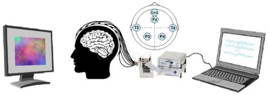
Figure 1.
Experimental setup: Screen, participant with electroencephalography (EEG) headset, EEG hardware acquisition system and PC. The electrodes positioning schema is presented on top.
2.3. Stimuli
Three types of images were used as visual stimulation, namely: Single color (Uni), natural color textures (Nat) and synthetic color fractal (Frac) images (Figure 2). The synthetic fractal images were generated with an algorithm which mimics the Brownian movement having as parameter the Hurst coefficient which controls the complexity [31], natural images as a comparison with known textures taken from the online Vistex database https://vismod.media.mit.edu/vismod/imagery/VisionTexture/vistex.html and single color based images, acting as a reference, generated as one uniform color based on the mean RGB color values of each Nat and Frac image, such as each R, G, B channel of the new Uni image was formed considering the mean of its representative R, G, B channel of a Nat or Frac image, plus adding small random variations for each RGB channel (), for variety, generating more Uni images. For example, the Uni image ⯀ (brown) corresponds to the mean RGB values of Figure 2a image, and ⯀ (grey) to Figure 2f image. In Figure 2, the complexity increases from left to right, relating to higher color content, important variation, randomness and irregularity [3,47]. The images were presented with a resolution of 512 × 512 pixels.
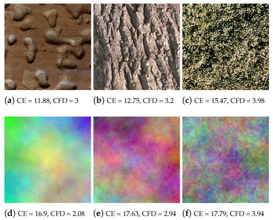
Figure 2.
Stimuli images examples: Top natural textures (Nat) and synthetic fractal textures (Frac) bottom.
2.4. Color Image Complexity Measures
As mathematical measures for characterizing complexity, we use Color Entropy (CE) [3,48] and Color Fractal Dimension (CFD) [31]. The color space used was RGB, consistent with both natural and synthetic fractal texture images used in our experiments.
2.4.1. The Color Entropy
The Color Entropy measures the disorder in signals [3,48], relating to the variation of signal values, while for images, to the variation in texture image colors, with no information on pixels spatial arrangement. The same definition is considered in this paper, with an extension to the multidimensional color case, as described in [3].
where is the probability of appearance of pixel value i in the image, and N the amount of possible pixel values.
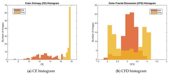
Based on the color entropy measure, the natural images selected for the experiment are comprised between 7.33–16.37 and fractal images between 16.45–17.84. Frac images exhibit higher complexity in colors compared to Nat images, as shown in the color entropy distribution in Figure 3a, meaning that the synthetic fractal images have higher variability in the color space.
2.4.2. Color Fractal Dimension
The most representative quantitative measure for expressing fractal geometry of color texture images is fractal dimension [3,49]. It expresses the variations and irregularities of a texture [50,51], as a relation to the self-similar regions observed across different size scales. The fractal dimension (Hausdorff dimension [52,53]) is estimated based on the probabilistic box-counting approach of [54], extended for the assessment of complexity of color fractal images with independent color components, as described in [7]. The spatial arrangement of the image (where the image is defined as a set of points S, (x,y,r,g,b)) is characterized by the probability matrix , the probability of having points included into a hyper-cube of size L (also called a box), centered in an arbitrary point of S. The scaling factor D (fractal dimension) is related to total number of boxes needed to cover the image:
where N is the number of pixels included in a box of size L, and m the amount of points contained in the box L. The extension of the Voss approach to color images [7] counts the number of pixels that fall inside a 3-D RGB cube of size L, using the Minkowski infinity norm distance, centered in the current pixel. The estimation of the regression line slope for the evolution of (log-log curve) is modified with a weighting function . The color fractal dimension D is then estimated using the robust fit approach with its 9 methods: ‘ols’ (least squares method), ‘andrews’, ‘bisquare’, ‘cauchy’, ‘fair’, ‘huber’, ‘logistic’, ‘talwar’, ‘welsch’, and the average over all estimations is considered as the CFD value. For more details, see [7,31].
From the point of view of entropy, the synthetic color fractal images exhibit a larger complexity as compared to color natural images, however, considering color fractal dimension, their complexity is similar, between 1.89–3.98 for natural images and between 2.03–4.12 for fractal images. As observed in Figure 3b, their complexity distributions intersect for the majority of the images (91.84%).
2.5. Experimental Session
The experimental session consisted in a 30 min session of visual stimulation which was split in 3 blocks with 5 min breaks in between and consisted in 560 trials (visual stimulation sequences) with the 3 types of images being randomly presented, on a grey background, with a ratio of 65:17:18% for Uni/Nat/Frac images. Each trial consisted in 3 parts: (i) attention (500 ms) where a white attentional cross is presented on grey background and acts as a preparatory and attention period for the actual stimulation/trial, attracting the sight in the center of the screen; (ii) trial (stimulus image) lasting for 1000 ms for block 1, 750 ms for block 2 and 500 ms for block 3, where the participant visualizes the image and has to think about its complexity and decide on its degree on a scale 1 to 3, from low to medium and high complexity by mentally pronouncing 1, 2 or 3, accordingly, and disregard the Uni images; and lastly, (iii) relaxation of 700 ms duration, where the participant relaxes the mind (Figure 4). First reaction on complexity was targeted, therefore the images were visualized for the first time during the stimulus presentation. Without any prior training or information provided on complexity definition and assessment, the decision and rules on complexity were left open to participants, which were requested not to change their reasoning process during the experiment.
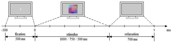
Figure 4.
Experimental paradigm and timing: fixation period of 500 ms, trial of 1000/750/500 ms for blocks, and relaxation period of 700 ms.
2.6. Material and Equipment
Signal acquisition: Biopac BioNomadix EEG wireless system (https://www.biopac.com/product/bionomadix-2ch-wireless-eeg-amplifier/) with 3 modules and 6 electrodes: P3, T3, Gnd, P4, T4, Fz, positioned according to the 10–20 international system and referenced to the ear lobes (see Figure 1). Stimuli presentation: SuperLab software and 20" LCD screen with 16:9 aspect ratio and 60 Hz refresh rate. Data acquisition: Acqknowledge software. Signal processing: Matlab along with the BBCI Matlab Toolbox (https://github.com/bbci/bbci_public) [55] and EEGLab (www.sccn.ucsd.edu/eeglab/) [56].
2.7. Participants
Eight voluntary participants took part in the study, 3 females and 5 males, BSc students and graduates in electronics engineering, ranging between 20–30 years old, with no experience in BCI experiments and little to no experience in imaging, photography or art. Participants received a priori information on the experiment and they expressed their consent to take part in the non-invasive experiment, and their permission for brain signals recording. The data was completely anonymized.
3. EEG Analysis
In this section, the processing steps are described which helps cleaning the signals from additional perturbations in order to enhance the SNR and give us information over the neurophysiological effects of perception, interpretation and cognition. For a complementary overview of the neural activity [57], we investigate not only the temporal responses (ERPs), but also the oscillations in the spectral domain (Power spectral density, PSD), as well the neural modulations given by (De)Synchronization (ERD/ERS) in order to observe how the frequency oscillations vary in time, which are investigated in more detail with Event-Related Spectral Perturbation (ERSP) which can capture all together the modulations within the entire frequency spectrum over time.
- Bad channels rejection (Participant-specific bad channels rejection and low quality channels rejection)—Firstly, bad quality data was removed from further analysis, such as bad signal quality due to poor conductance, e.g., signal amplitude > 300 V. Further, channels were checked for variance dropping to zero and removed if positive (criterion: variance < 0.5 in more than 10% of trials [58,59].
- Filtering—we applied low-pass and high-pass filtering. For lowpass filtering, used for anti-aliasing, we applied the Chebyshev type II filter of order 10 with 42 Hz pass-band edge frequency and 3 dB ripple, and a 49 Hz stopband with 50 dB attenuation. The high-pass filter, used to reduce drifts, was applied with a 1 Hz FIR filter of order 300, using least-squares error minimization and reverse digital filtering with zero-phase effect, such as not to induce phase delays.
- Artifact rejection—For the purpose of rejecting non-EEG origin components (ocular, muscular, cardiovascular, etc.), Independent Component Analysis (ICA) with Multiple Artifact Rejection Algorithm (MARA) based on feature selection [60] were used.
- Segmentation—Data was segmented in epochs, where one epoch corresponds to one stimulation sequence.
- Epochs rejection—Noisy trials were removed based on a variance criterion, such as the ones greater or equal then a trial threshold per channels (where in 20% of the channels have excessive variance). Further, artifactual trials were rejected based on max-min criterion, such as the difference between the maximum and minimum peak should not exceed a threshold, e.g., 150 V.
- Baseline correction—For each epoch, the mean of the last hundreds of ms from the attentional period is subtracted from the epoch, either in the time or frequency domains, aiming at diminishing the background neural noise activity [61].
- Grand Average (GA)—All trials have been averaged over all participants for neurophysiological interpretation, and investigated in the temporal and frequency domains. Scalp maps distributions of the brain signals will also be presented, where a shading method based on linear interpolation between neighbor channels is used to get smooth plots (available via BBCI Toolbox, [55]).
- (a)
- Event-Related Potential, ERP analysis—For ERP analysis, the temporal signals are investigated and averaged on all signals over all participants. For baseline correction, the last 100 ms are used from the attentional period.
- (b)
- Signed and squared point biserial correlation coefficient measure (signed )—For details on the association strength between the brain responses for different perceptions, the signed and squared point biserial correlation coefficient (signed ) [62] is computed separately for each pair of channel and time point (x), over all epochs, as in [63], being proposed by [64] (see Equation (3)).where n1 and n2—the numbers of samples in class 1 and class 2, respectively, i,1 and i,2 the class means and the standard deviation, while the signed values are sgn-r(x) = sign(x) r(x). It is a measure of how much variance of the joint distribution can be explained by class membership.
- (c)
- Event-Related (De)Synchronization, ERD/ERS analysis—The neural modulations in different frequency bands, such as the (de)synchronization (ERD/ERS) effects [43], are outlined by the modulation of the amplitudes in the temporal domain, such as the signals envelopes within specific chosen bands. We used the upper envelope computed based on the Hilbert Transform [65] and then smoothed with a moving average filter based on the Root Mean Square (RMS) with a 200 ms sliding window. The envelope is baseline corrected using an interval of 200 ms from the fixation period.
- (d)
- Power spectral density (PSD) analysis—The power spectrum from 3 to 40 Hz, is computed on the trial interval (0–1350 ms), based on the Fourier transform with Kaiser window (Smith, 1997) and the logarithmic spectral power is presented as .
- (e)
- Event-Related Spectral Perturbation (ERSP) analysis—In addition to the narrow-bands ERD curves, the Event-Related Spectral Perturbations (ERSPs) method allows the simultaneous investigation of the full spectrum [57,66,67,68]. Computed here (with EEGLab) based Short-Time Fourier analysis using Morlet wavelet transform with three cycles wide windows at each 0.5 frequency, within 0–50 Hz, on the interval −550 ms to 1350 ms, relative to the baseline period (−200, 0 ms).
- (f)
- Inter-Trial Coherence, ITC—In contrast to ERSP, Inter-Trial Coherence (ITC) offer additional information over the local phase coherence across consecutive trials [69], since the ERD/ERS phenomena are time locked to a stimulus, not phase locked to an event [57,70].
- Classification—We are interested to investigate if the brain responses can be discriminated in accordance to the image perceived, namely the synthetic fractal texture, Frac, the natural texture Nat, or the reference image, Uni. The estimation is performed using single-trial classification, by Regularized Linear Discriminant Analysis [71], in multi-class form. The three class labels are given by the stimuli images: Uni, Nat or Frac. Spatio-temporal features (channels and time, extracted as in [30,64]) are considered from intervals with highest discriminations between classes based on the signed . Namely, the signed discriminability is computed between Nat–Uni and Frac–Nat classes on the temporal signals (0–1200 ms) for all channels, and three short intervals of up to 150 ms are heuristically selected for each discrimination pair (Nat–Uni and Frac–Nat) where the discriminability is highest across all channels (see Section 4). The short temporal intervals detected are comprised within the 200–400 ms and 480–1200 ms ranges. The averaged value of the temporal signals within these short intervals considering each channel and each discrimination pair is further selected for each trial, giving a concatenated vector as spatio-temporal features of 6 × 5 dimension: 3 averaged values for Nat–Uni pair, 3 for Frac–Nat pair, for all 5 channels and all trials. Separately, also multi-modal classification is investigated considering frequency features along with the temporal features (spatio-tempo-spectral features). Similarly, the spectral features are detected as averaged values of the power spectrum (0–30 Hz) within three frequency intervals with maximum signed discriminability over the power spectrum (3–40 Hz) for Nat–Uni and Frac–Nat pairs. The frequency range intervals selected vary around 8–14 Hz and 17–39 Hz, consistent with the highest spectrum differences as observed in spectrum analysis in Section 4. The multi-modal features consider temporal features from the parietal area (P3, P4) and spectral features from the temporal area (T3, T4), giving a concatenated feature vector of 6 × 4 dimension: 3 temporal averaged values for Nat–Uni, 3 temporal for Frac–Nat, 3 spectral averaged values for Nat–Uni, 3 spectral for Frac–Nat, considering 4 channels (T3, T4, P3, P4). For validation, 3-folds cross-validation is used, where the data set is split in 3 parts, one used for training and 2 for testing, and the classification is repeated until each part has been used as training [72]. The classifications are evaluated with normalized loss (Equation (4)), which helps with weighting for unbalanced classes. The normalized loss is a ratio out of 1, therefore the performance (the accuracy, Acc) is given by: Acc = 1–loss. The final classification performance is computed as the average accuracy over all folds.where n is the number of classes such as , is the number of wrongly estimated samples in class i, and the number of samples in class i.
4. Experimental Results
In this section, we present the results of time and frequency analysis which bring complementary information over the neural oscillations measured by EEG.
In terms of participant’s mood, the experiment scenario did not produce influences and it remained approximately the same during and after the experiment, stated by each participant at the end of the experiment. Half of the participants stated higher complexity for Nat images as compared to Frac images, one participant categorized Frac images as more complex, and the rest considered equal complexity. As for the difficulty of decision, 5 participants rated Nat images as more difficult to evaluate, one Frac images and 2 as equal difficulty. Moreover, participants stated that in some cases they were unintentionally still thinking over the images complexity, even after the stimulus interval, even though they were requested to only relax in the relaxation period. A quarter of participants associated the natural images content with known objects, even though we have done our best to avoid this fact when we selected the natural images, such as to restrict thinking to the structural form and not to trigger memory.
Considering signals investigation, it is important to note that the stimulus software and the wireless hardware introduced a constant delay of approximately 150 ms in the signal due to communication between sensors and acquisition system, after the start of the trial (time: 0 ms). Therefore, this delay has to be considered when interpreting the observed responses.
After the channels and artifacts rejection steps, no channels were rejected and 21 epochs on average were removed with a ratio of 0.65:0.11:0.24 from the Uni, Nat and Frac classes. No artifactual components were detected and removed after ICA, mainly because of less spatial information available due to the small number of channels and also missing pre-frontal and EOG electrodes, which could’ve captured better the eye movements, for example.
4.1. Event-Related Potentials (ERPs)
The neural fluctuation over the perception of images is shown in Figure 5, which show the averaged brain signals in the time domain, across all epochs, for channel P3. For an overview of all channels, see Figure A2 in Appendix A. Even though, the experiment was performed with 3 different blocks of visual stimulation, each having a different stimulation duration (block 1:1000 ms; block 2:750 ms; block 3:500 ms), the grand average responses are similar, see Figure A1 in Appendix A. Hence, the ERPs are visually investigated considering all blocks together. In more detail, Figure 5, shows the temporal evolution of the grand average ERP responses, complemented with their spatial evolution. The grey horizontal line marks the start of the trial period (0 ms) which lasts for 500 ms minimum, followed by the relaxation period (750 ms). When looking at the brain responses over time, we can easily observe 2 distinct groups of strong peaks, one at 300–600 ms, representing the well-known P200 and P300 components and another group later around 800–1200 ms, as an effect to the visual response over the non-informal grey image within the relaxation period, indicating prolonged cognition, with both groups of peaks being more prominent for the parietal area at P3 and P4 channels, which is responsible for cognitive reasoning. We observe the same latency and duration of the averaged ERP peaks for all 3 types of images perception, with differences in amplitude, such as:
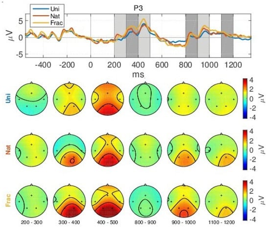
Figure 5.
Grand Average (GA) Event Related Potential (ERP) and scalp topographies over all blocks for channel P3. The scalp topographies relate to the temporal intervals shaded in grey.
- (i)
- a slight decreased N200 peak for Uni images (at 250 ms), relating to visual perception [73];
- (ii)
- a gradually increased amplitude already from the P200 (350 ms), as response to an increase in image complexity perception from Uni to Nat and Frac images perceptions, observed also spatially (see scalp plots in Figure 5) with increased activity in the parietal area (P3, P4 channels), highest for fractal images perception (3 V);
- (iii)
- even higher amplitude for the P300 (at 450 ms) towards 4 V in the parietal area, as compared to P200.
- (iv)
- the second group of peaks around 800–1100 ms, with similar amplitude and spatial distribution for P200 in the parietal area (at 850 ms, appearing 350 ms after the grey image presentation), followed by another peak (950 ms, 450 ms after the grey image presentation) with gradually increased amplitude for Uni, Nat and Frac images of up to (2–3 V), focused in the right parietal area. This relates to an extended reasoning process, since participants stated that they were unintentionally still thinking over the image complexity, even after the stimulus interval, even though they were requested to only relax in the relaxation period.
Moreover, the ERPs discriminations are highlighted by the signed measure, as shown in Figure 6 for channel P3, and class groups (Nat–Uni, Frac–Nat) where a value of zero of the signed indicates no correlation between the classes and a positive value indicates that the amplitude was larger for the first class in the group than for the second class and vice versa for negative values. We observe higher correlation over trials in time in the parietal area for Nat–Uni discriminability (Figure 6a) of up to within 300–400 ms, 800–900 ms, and 1150–1250 ms intervals, while for 500–600 ms the distribution is viewed across the entire brain (see scalp plots in Figure 6a). Similarly, the Frac–Nat discriminability in Figure 6b show higher parietal differences for the 300–400 ms, 500–600 ms, and 1150–1250 ms intervals. The signed differences are higher between Nat and Uni, compared to Frac and Nat images perceptions.
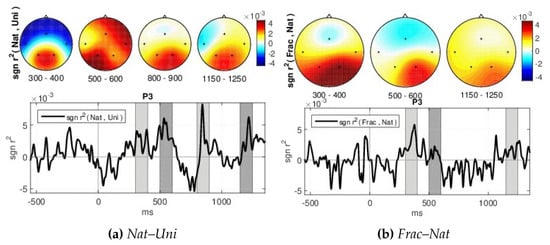
Figure 6.
GA signed over all blocks for: (a) Nat–Uni and (b) Frac–Nat discriminations at P3 channel.
4.2. Event-Related (De)Synchronizations, ERDs/ERSs
When analyzing the amplitude envelopes evolution over time for different frequency intervals within 3–40 Hz, we notice the highest differences between classes (0.5–1 V) within the (8–14 Hz) and (20–28 Hz) frequency bands, shown in Figure 7. The envelopes are similar until the 300 ms time point, corresponding to the same type of processing the external information (visual perception). First a synchronization event (ERS) > 0 V starts at 200 ms, more pronounced for the parietal sites (P3 and P4) within 8–14 Hz (Figure 7a), followed by desynchronization, deeper at 500 ms, expressed by decreased amplitudes (<0 V), which corresponds to a preparation of a higher complexity task (evaluating images complexity in case of Nat and Frac classes). Further, an amplitude increase follows from 600 ms, producing synchronization at 1000 ms within the band. More pronounced desynchronization is modulated by more complex cognitive processing, for Nat and Frac perceptions, compared to Uni image perceptions where no cognition is involved, highest for the parietal sites. While between Nat and Frac image perceptions, the envelopes evolutions tend to be similar before 600 ms, and differ in synchronization, higher for Frac perception (see P4 within band at 1000 ms and P4, T4, T3 within band, even from 400 ms onwards). The variations in amplitude at 500 ms and 1000 ms time points correspond to the ERP peaks.
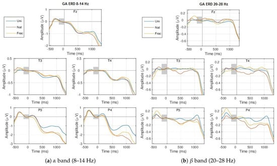
Figure 7.
GA ERDs over all blocks, for the 3 types of images: Uni (blue), Nat (red), Frac (orange), considering all channels and the: (a) (8–14 Hz) and (b) (20–28 Hz) frequency bands. The shaded grey area marks the considered baseline period (−200,0) ms.
Details on the spatial activity of the neural modulations in the (8–14 Hz) and (20–28 Hz) bands can be seen in Figure A3 in Appendix A.
4.3. Power Spectrum
Looking at the strength of the GA power spectrum on the 3–40 Hz frequency interval (Figure 8a), we notice higher power for Uni perception for the band (8–12 Hz) for all channels (Figure 8b) and lower for the perception in the and bands, between 20 Hz and 35 Hz for the temporal channels (Figure 8c). The effect is in line with the literature stating that more complex processes decrease in frequency. The fact that the parietal sites do not show visible differences in higher bands for Nat and Frac perceptions might relate to the fact that the thought process of evaluating images complexity is comparable. The visible differences in frequency for the temporal sites might indicate, access to memory, since it’s natural for the human mind to correlate forms and structures with already known objects [74,75]; process which is easier for Nat images since they represent natural textures and they are recognizable to some extent (as stated by subjects). While for Frac images perception, the correlation is far to be straightforward and if one would imagine a recognizable form, the thought process will be more difficult (therefore the decrease in power in the temporal sites, more pronounced for Frac images, in Figure 8c). For example, one subject specified that for Frac images he was thinking at sand grains; but of course, for a conclusion to be made, this fact need to be analyzed separately in a study on each subject, relating to its exact thought process.
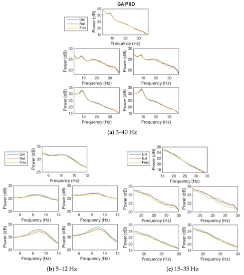
Figure 8.
GA Power Spectrum over all blocks, for Uni (blue), Nat (red) and Frac images (orange), for all channels, on: (a) 3–40 Hz, (b) 5–12 Hz, (c) 15–35 Hz.
For more details on the neural modulations modulations within different frequencies over time, as related to perception and decision-making, see the Event-Related Spectral Perturbations (ERSP) investigation in Figure A4, Figure A5 and Figure A6 in Appendix A.
4.4. Classification
In Figure 9, the distribution of the classifier performance is presented for all participants and data folds, in form of box plots (where top and bottom box plot edges represent the 75 and 25 percentiles, whiskers show the min and max values, the median is indicated by the horizontal red line and the mean by the black asterisk). The statistical significance is represented above each box plot, where ‘**’ marks significance at 0.01 and ‘*’ at 0.05. The chance level of 33%, such as for 3 classes, is highlighted by the horizontal dotted line.
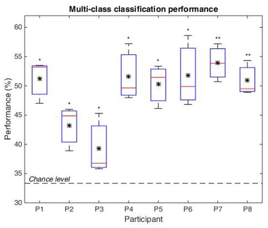
Figure 9.
Multi-class classification performance (Uni, Nat, Frac) for each participant, considering the three folds. The box-plots consider the 25% and 75% percentiles, the the black asterisk represents the mean values and the red horizontal line is the median.
Considering multi-class classification on the temporal features, the average classification performance is 49%, significantly over chance level (given by t-test at = 0.0001), with the lowest mean accuracies for participants P3 and P4: Acc(P3) = 39.3% and Acc(P4) = 43.3% (as seen in Figure 9). For the remaining participants the performances exceed 50%, statistically significant with t-test at 5% significance level, and even at 1% significance level for P7 and P8 with highest performances over all folds.
When analyzing the performance within classes, very good performances are likewise obtained in each case, with a mean 52.81% accuracy for multi-class classification. The confusion matrix of last classification fold is presented in Table 1, where the rows relate to the target class, and the columns to the classifier output). The diagonal shows the percentage of correct classified epochs in each class (55.3% for Uni, 53.5% for Nat and 49.6% for Frac), statistically significant over the chance level of 33.33%. The miss-classified trials for Nat and Frac classes (25.1–26.9%) tend to be higher then for Uni class (21.5–23.5%), which might relate to the higher amplitude difference within trials between Nat or Frac classes, as compared to Uni, and smaller between Nat and Frac classes; even though, the percentage difference between miss-classifications is not significant to support this conclusion.

Table 1.
Normalized mean confusion matrix (in %) for multi-class classification on the last fold.
In addition, since the differences obtained in the spectral domain bring additional information (as shown in [30,76]), we have performed also multi-modal classification integrating also spectral features in addition to temporal features, in a complementary scenario, considering temporal features (from P3, P4) and spectral features (from T3, T4). However, the classification performance did not improve significantly: 52.46% for Uni, 54.21% for Nat, 53.24% for Frac (ns. with t-test at = 0.05, p = 0.5324, p = 0.8817, p = 0.2872). The effect of no considerable improved performance might be due to the fact that compared to the temporal case, smaller differentations are observed between classes in the spectral domain (<1 dB) which does not improve much the classification.
5. Discussion, Conclusions and Future Work
We performed the presented preparatory experiments to get insights into the human brain perception of synthetic color fractal and natural textures and the freely reasoning over the images complexity, all by using a less informative EEG setup, in order to form the ground basis for a more in-depth study and investigate if a less channels EEG system is able to provide any reliable information on visual perception and reasoning of image complexity. We quested to find and quantify any differences between the preliminary perception of synthetic color fractal and natural textures with EEG in short intervals up to 1 s.
Firstly, the analysis showed that the fractal images may constitute stimuli for more throughout studies, while due to their capturing properties we could investigate their capacity to induce brain oscillations, and even further they presented interest for the participants.
In more detail, the observed neurophysiological facts in the ERPs suggests that the primary visual processing of the stimuli (P200) is differentiated for the three types of images (Uni, Nat, Frac), while the perception, interpretation and reasoning over the complexity of textures (P300), shows higher discriminability involving different thought processes. The gradual increased amplitude ERP responses currently observed tend to be related to more complex processes and stronger attentional demand, as reported in the scientific literature [29].
Even though the texture complexity does not vary according to the CFD measure between Nat and Frac images, but only the amount of colors as indicated by color entropy (CE), perceiving the complexity of fractal images by the human brain seem to require more thought processes. These could relate to the higher number of colors for fractal images, or the irregular synthetic structure unrelated to any known forms, which probably makes it harder for the brain to create rules for complexity differentiation. Increased brain parietal ERP activity suggests increased difficulty as with higher information load [77], which differ depending on the content and structure of the textural image. This effect is further highlighted by the decreased ERDs at parietal sites (more complex processing) and slightly higher at temporal sites (due to the recognizable distinction between Nat and Frac), which gradually decreases as with increased image complexity perception from Uni to Nat and Frac. The natural images generate desynchronizations even in higher frequencies such as band, which tends to imply, a more intense process, as compared to fractal images. This may be to the fact that natural images contain more detailed structures which generates a profound thought process for establishing logical connections and criteria for complexity levels differentiation, while for the synthetic abstract fractal structures, the differentiation is either done automatically by subconscious processes or is ambiguous. This is supported by participants opinion, where 5 participants stated a more complex decision for natural images. After an overview of the neural responses, it seems that, generally, the thought process of evaluating natural images complexity is more complex than in the case of fractal images, requiring more processes, while the fractal images complexity perception probably induces a more intense reasoning process, causing more neurons to fire, adding up to the ERP potential, by probably accessing a deeper reasoning with respect to a detection of imaginatory forms for differentiation. While on natural textures, the complexity decision might easily relate to known structure and form types, for synthetic fractal textures it is harder to relate to known structures, even though the complexity evaluation has been shown in the experiment to be easier. In more detail, from the observers’ point of view, half of the participants considered the structure of the natural images as more complex compared to the fractal ones, which might indicate more entangled structures for the natural images case. More, since the complexity decision was freely-open to participants, the thought processes and criteria used play an important role in reasoning, which may activate different parts of the brain, therefore grouping participants further based on reasoning will be a good choice.
The findings are enforced by the fact that even there is no difference between the number of occurrences of the presented natural and fractal images, and similar range in complexity degree according to CFD, a noticeable difference is still observed in the brain signal representations. Regardless of the cause that triggered the neural responses differentiation, good classification discrimination between Nat, Frac and the reference Uni are obtained. Despite the fact that the combined temporal-spectral classification did not provide higher performances, the complementary information can be taken into account by adapting the classifier on each participant, to the most discriminative features either in time or frequency, to take advantage of the physio-anotomical differences between individuals and different thought processes which produce distinct neural effects.
Further, we plan to investigate in more depth the perception over the complexity degrees, to see whether different complexity levels within images can induce distinct brain responses. This should be investigated not only on grand average, but also within each participant, since each individual has its own perception over complexity, as noticed in this study.
For a more in-depth view over perception, the future studies should consider more participants for an expansive overview (at least 15, as proved statistically [78]) and more channels to better capture the spatial activity in detail. Considering hardware, a system with active electrodes will be advantageous to better filter the noise and have better signal conductance, while targeting practical applications the WiFi property have to be kept and dry electrodes would be better suited [79]. Considering timing, maybe a longer Inter-Stimuli Interval (ISI) should be considered for the future studies to capture all reasoning processes steps, while extended thought processes over complexity prolonged also in the relaxation period, as seen in this study. Further the neural fluctuations in an overt scenario [80], where participants can freely scan an image, will be interesting to be investigated.
For pointing out the fractal complexity itself, in a natural-synthetic textural scenario, integrating also fractal natural images and similar synthetic generated textures, will be a good comparison, to have similar complexity ranges, fractal structures and textural variations. Here, we considered natural non-fractal images for the moment, due to the limited availability of a standardized diverse data base of natural fractal images with same image captured conditions (e.g., light, angle, distance to object). For the future, we consider creating our own dataset. The higher activity in the later interval even after the end of the presented image, suggests a complex and a prolonged continuous background process which may also indicate a delay in decision making. This aspect should be captured in the trial-by-trial variability and separately between subjects by looking over the latency and duration of the potentials. If this is the case, ERPs should elicit late positivity with high amplitude [81] and ongoing negative ERP over the prefrontal cortex suggesting indecisiveness [82]. Since natural images represent recognizable structures and objects, as compared to unidentified forms for the synthetic fractal images, it might infer different reasoning mechanisms. In neuroscience, it is suggested that the sensory cortex may have adapted to statistical regularities and therefore automatically relax, reducing attention [83]. At higher levels of abstraction, non repetitive and novel stimulus would trigger more attentional processes [84]. In our stimulus setup, the synthetic fractal images were more consistent having similar structure, while the natural textures were more various. Further, it has been shown that the ratings of complexity are influenced significantly with judgments of familiarity [85]; recognizable forms that are easily categorized reduce the complexity of the texture and brain’s interpretation becomes easier. Such as, with an increased familiarity, observers will overcome any complexity effects, resulting in shorter latencies. On the other hand when something is less likely, it will require more pieces of information to determine its meaning, hence longer latencies. Even though we tried to eliminate as possible recognizable textures from the natural image set, the familiarity effect still has an influence. These possible discrepancies given by distinctive regularities structures and familiarity influences should be eliminated in the next in-depth study.
Characterizing texture plays an important role in computer vision in expressing the characteristics of a surface, while better understanding perception can be of great use for multimedia quality assessment by relating to the internal mechanisms of the human visual system, while for out of the lab applications, practicality is important. Therefore, in these prior experiments we investigated if a shallower information system (less channels) can capture aspects of complexity perception and reasoning, targeting real life applications where a bulky system will obstruct an easy use. We observed that even with 5 neural channels some information can still be captured and the complexity perception of synthetic color fractal and natural textures can be discriminated via LDA classification.
Author Contributions
Conceptualization, I.E.N. and M.I.; methodology, I.E.N. and M.I.; software, I.E.N.; validation, M.I.; formal analysis, I.E.N.; investigation, I.E.N.; resources, M.I.; data curation, I.E.N. and M.I.; writing—original draft preparation, I.E.N.; writing—review and editing, M.I.; visualization, I.E.N. and M.I.; supervision, M.I.; project administration, M.I.; funding acquisition, I.E.N. and M.I. All authors have read and agreed to the published version of the manuscript.
Funding
The current work is part of the post-doctoral research project entitled PerPlex: “Human brain perception on the spatio-chromatic complexity of fractal color images”, carried out at University Transilvania of Brasov (UniTBv), Romania and was funded by the National Council of Scientific Research (CNCS) Romania via CNFIS-FDI-2019-0324.
Institutional Review Board Statement
All procedures performed in the study involving human participants were approved by the relevant ethical committee of Medical Electronics and Computing Laboratory from the Faculty of Electronics, Telecommunications and Information Technology, University Politehnica of Bucharest in accordance with the 1964 Helsinki declaration and its later amendments or comparable ethical standards.
Informed Consent Statement
Informed consent was obtained from all individual participants included in the study and the recorded data is completely anonymized.
Data Availability Statement
The recorded EEG data is available at http://dx.doi.org/10.6084/m9.figshare.13489215 [86].
Acknowledgments
We thank the reviewers for their valuable comments and revision on an earlier version of the manuscript which helped improved the present manuscript.
Conflicts of Interest
The authors declare no conflict of interest. The funders had no role in the design of the study; in the collection, analyses, or interpretation of data; in the writing of the manuscript, or in the decision to publish the results. No copyright issues are declared for all images.
Appendix A
Appendix A.1. Additional Graphs
Appendix A.1.1. GA ERPs
Figure A1 show the temporal evolution of the ERPs as comparison between the three blocks. No important difference is observed in the latency of the ERP peaks between blocks.

Figure A1.
GA ERP over blocks for channel P3.
The GA ERPs for all 5 recorded neural channels: Fz, T3, T4, P3, P4 is shown in Figure A2.

Figure A2.
GA ERP responses over all blocks, for the 3 types of images: Uni (blue); Nat (red); Frac (orange), considering all channels. (Please note that temporal sites channels (T3 and T4) will appear nosier in the graphics, while their conductivity was lower compared to the other channels, since they were a bit loose during experiments due to their placement on the EEG cap lateral sides.)
Appendix A.1.2. Event-Related (De)Synchronization, ERD/ERS
The scalp plots in Figure A3 show decreased ERDs at parietal sites and slightly higher at temporal sites, which gradually decreases as with increased image complexity and perception from Uni to Nat and Frac. The activity in the the band (Figure A3b) tends to become synchronized in the frontal area for Nat and Frac perceptions referring to the thought process itself of evaluating images complexity. Comparing between bands, stronger ERDs/ERSs down to −3 V are noticed in the band Figure A3a, and weaker between V and V in the band Figure A3b.

Figure A3.
GA ERDs over all blocks, for Uni (blue), Nat (red) and Frac images (orange), within the: (a) (8–14 Hz) and (b) (20–28 Hz) frequency bands, considering the P4 channel.
Appendix A.1.3. Event-Related Spectral Perturbations, ERSP
In Figure A4, Figure A5 and Figure A6, the spectral perturbations are presented highlighted by bootstrapping at = 0.01 level, where no significant points are presented in green. For the top plots, the right color bar shows the scale of the power spectral density (−2.2 dB); the lateral left panel shows the baseline mean power spectrum; the lower panel show the ERSP envelopes (low and high mean dB values, relative to baseline, at each time in the epoch, across all frequencies). Bottom plots show the Inter-Trial Coherence (ITC), where the right color bar shows the coherence strength scale (ITC values); the left panel shows the ITC frequency mean (blue trace) and ITC significance limits at each frequency (green trace); and the panel underneath shows the mean ERP trace.
Uni perception (Figure A4): The ERSP in the left parietal side (P3) show desynchronizations in the early interval (0–200 ms), and also later after 600 ms for up to 22 Hz and weaker beyond 22 Hz. The ITC measure ranges from zero to one for a specific time-point, explicitly from no synchronization between the EEG epochs to strong synchronization. For a given frequency range, it provides the magnitude and phase of the spectral estimation. It shows here that trials are phase-locked at 850 ms for up to 20 Hz, corresponding to the second group of P200–P300 peaks, a time-locked response relating effectively to visual processing for the grey image presentation event.

Figure A4.
ERSP over all blocks for Uni perception at P3 and T4, bootstrap significance level = 0.01.
Nat perception (Figure A5): The desynchronizations are stronger and extended in frequency and time, more pronounced in the frequency (over 30 Hz) for the T4 channel as compared to Uni image perception. For parietal site, lower ERDs are observed after 600 ms including also band. Considering ITC, no phase synchronization between trials is observed for the first group of P200–P300 peaks, since it includes the thought process of perception which is different between image to image.

Figure A5.
ERSP over all blocks for Nat perception at P3 and T4, bootstrap significance level = 0.01.
Frac perception (Figure A6): For fractal perception, the strong desynchronizations continue until 30 Hz for P3, after 600 ms, and until 20 Hz for T4 after 600 ms. Synchronization is also observed for T4 at 250–450 ms in the band (20–30 Hz), effect significant as detected by bootstrap statistics at 0.01 confidence level.
Comparing between Uni, Nat and Frac images perceptions, the effects tend to suggest a more complex cognitive process for Nat perception, with extended ERDs in higher bands and not significant for Frac perception in the parietal sites. While significant and extended ERDs in and observed for Nat perception in the temporal area, with only in (>30 Hz) for Frac perception, tend to indicate higher memory recall activity for Nat and intensive for Frac images. The representative perturbations in the frequency band relate to attention and an easier processing, while in addition, the significant beta and gamma modulations represent more complex mental activity [87]. The strong synchronization within the baseline period (−400, −200) ms relates to a time-locked visual response to the attentional image, process identical in all three cases.

Figure A6.
ERSP over all blocks for Frac perception at P3 and T4, bootstrapping = 0.01.
References
- Zoefel, B.; VanRullen, R. Oscillatory mechanisms of stimulus processing and selection in the visual and auditory systems: State-of-the-art, speculations and suggestions. Front. Neurosci. 2017, 11, 2–96. [Google Scholar] [CrossRef] [PubMed]
- Yadav, A.K.; Roy, R.; Kumar, A.P. Survey on content-based image retrieval and texture analysis with applications. Int. J. Signal Process. Image Process. Pattern Recognit. 2014, 7, 41–50. [Google Scholar] [CrossRef]
- Ivanovici, M.; Richard, N. Entropy versus fractal complexity for computer-generated color fractal images. In Proceedings of the 4th CIE Expert Symposium on Colour and Visual Appearance, Prague, Czech Republic, 6–7 September 2016; pp. 432–437. [Google Scholar]
- Kisan, S.; Mishra, S.; Mishra, D. A novel method to estimate fractal dimension of color images. In Proceedings of the 2016 11th International Conference on Industrial and Information Systems (ICIIS), Roorkee, India, 3–4 December 2016; pp. 692–697. [Google Scholar]
- Zunino, L.; Ribeiro, H.V. Discriminating image textures with the multiscale two-dimensional complexity-entropy causality plane. Chaos Solitons Fractals 2016, 91, 679–688. [Google Scholar] [CrossRef]
- Forsythe, A.; Nadal, M.; Sheehy, N.; Cela-Conde, C.J.; Sawey, M. Predicting beauty: Fractal dimension and visual complexity in art. Br. J. Psychol. 2011, 102, 49–70. [Google Scholar] [CrossRef]
- Ivanovici, M.; Richard, N. Fractal dimension of color fractal images. IEEE Trans. Image Process. 2011, 20, 227–235. [Google Scholar] [CrossRef]
- Jones-Smith, K.; Mathur, H. Revisiting Pollock’s drip paintings. Nature 2006, 444, E9–E10. [Google Scholar] [CrossRef]
- Ivanovici, M.; Coliban, R.M.; Hatfaludi, C.; Nicolae, I.E. Color Image Complexity versus Over-Segmentation: A Preliminary Study on the Correlation between Complexity Measures and Number of Segments. J. Imaging 2020, 6, 16. [Google Scholar] [CrossRef]
- Morabito, F.C.; Cacciola, M.; Occhiuto, G. Creative brain and abstract art: A quantitative study on Kandinskij paintings. In Proceedings of the 2011 International Joint Conference on Neural Networks, San Jose, CA, USA, 31 July–5 August 2011; pp. 2387–2394. [Google Scholar]
- Morabito, F.C.; Morabito, G.; Cacciola, M.; Occhiuto, G. The Brain and Creativity. In Springer Handbook of Bio-/Neuroinformatics; Springer: Berlin/Heidelberg, Germany, 2014; pp. 1099–1109. [Google Scholar]
- Donderi, D.C. An information theory analysis of visual complexity and dissimilarity. Perception 2006, 35, 823–835. [Google Scholar] [CrossRef]
- Donderi, D.C. Visual complexity: A review. Psychol. Bull. 2006, 132, 73. [Google Scholar] [CrossRef]
- Yu, H.; Winkler, S. Image complexity and spatial information. In Proceedings of the 2013 Fifth International Workshop on Quality of Multimedia Experience (QoMEX), Klagenfurt am Wörthersee, Austria, 3–5 July 2013; pp. 12–17. [Google Scholar]
- Ciocca, G.; Corchs, S.; Gasparini, F. Complexity perception of texture images. In International Conference on Image Analysis and Processing; Springer: Berlin/Heidelberg, Germany, 2015; pp. 119–126. [Google Scholar]
- Corchs, S.E.; Ciocca, G.; Bricolo, E.; Gasparini, F. Predicting complexity perception of real world images. PLoS ONE 2016, 11, e0157986. [Google Scholar] [CrossRef]
- Gartus, A.; Leder, H. Predicting perceived visual complexity of abstract patterns using computational measures: The influence of mirror symmetry on complexity perception. PLoS ONE 2017, 12, e0185276. [Google Scholar] [CrossRef] [PubMed]
- Matveev, N.; Sherstobitova, A.; Gerasimova, O. Fractal analysis of the relationship between the visual complexity of laser show pictures and a human psychophysiological state. SHS Web Conf. 2018, 43, 01009. [Google Scholar] [CrossRef]
- Guo, X.; Asano, C.M.; Asano, A.; Kurita, T.; Li, L. Analysis of texture characteristics associated with visual complexity perception. Opt. Rev. 2012, 19, 306–314. [Google Scholar] [CrossRef]
- Madan, C.R.; Bayer, J.; Gamer, M.; Lonsdorf, T.B.; Sommer, T. Visual complexity and affect: Ratings reflect more than meets the eye. Front. Psychol. 2018, 8, 2368. [Google Scholar] [CrossRef] [PubMed]
- Babiloni, C.; Vecchio, F.; Bultrini, A.; Luca Romani, G.; Rossini, P.M. Pre-and poststimulus alpha rhythms are related to conscious visual perception: A high-resolution EEG study. Cereb. Cortex 2006, 16, 1690–1700. [Google Scholar] [CrossRef] [PubMed]
- Demiralp, T.; Bayraktaroglu, Z.; Lenz, D.; Junge, S.; Busch, N.A.; Maess, B.; Ergen, M.; Herrmann, C.S. Gamma amplitudes are coupled to theta phase in human EEG during visual perception. Int. J. Psychophysiol. 2007, 64, 24–30. [Google Scholar] [CrossRef]
- Busch, N.A.; Dubois, J.; VanRullen, R. The phase of ongoing EEG oscillations predicts visual perception. J. Neurosci. 2009, 29, 7869–7876. [Google Scholar] [CrossRef]
- Hagerhall, C.M.; Laike, T.; Taylor, R.P.; Küller, M.; Küller, R.; Martin, T.P. Investigations of human EEG response to viewing fractal patterns. Perception 2008, 37, 1488–1494. [Google Scholar] [CrossRef]
- Acqualagna, L.; Bosse, S.; Porbadnigk, A.K.; Curio, G.; Müller, K.R.; Wiegand, T.; Blankertz, B. EEG-based classification of video quality perception using steady state visual evoked potentials (SSVEPs). J. Neural Eng. 2015, 12, 026012. [Google Scholar] [CrossRef]
- Grummett, T.; Leibbrandt, R.; Lewis, T.; DeLosAngeles, D.; Powers, D.; Willoughby, J.; Pope, K.; Fitzgibbon, S. Measurement of neural signals from inexpensive, wireless and dry EEG systems. Physiol. Meas. 2015, 36, 1469. [Google Scholar] [CrossRef]
- Mustafa, M.; Guthe, S.; Magnor, M. Single-trial EEG classification of artifacts in videos. ACM Trans. Appl. Percept. (TAP) 2012, 9, 1–15. [Google Scholar] [CrossRef]
- Portella, C.; Machado, S.; Arias-Carrión, O.; Sack, A.T.; Silva, J.G.; Orsini, M.; Leite, M.A.A.; Silva, A.C.; Nardi, A.E.; Cagy, M.; et al. Relationship between early and late stages of information processing: An event-related potential study. Neurol. Int. 2012, 4, e16. [Google Scholar] [CrossRef] [PubMed]
- Polich, J. Updating P300: An integrative theory of P3a and P3b. Clin. Neurophysiol. 2007, 118, 2128–2148. [Google Scholar] [CrossRef] [PubMed]
- Nicolae, I.E.; Acqualagna, L.; Blankertz, B. Assessing the depth of cognitive processing as the basis for potential user-state adaptation. Front. Neurosci. 2017, 11, 548. [Google Scholar] [CrossRef]
- Ivanovici, M. Fractal Dimension of Color Fractal Images With Correlated Color Components. IEEE Trans. Image Process. 2020, 29, 8069–8082. [Google Scholar] [CrossRef]
- Tononi, G.; Edelman, G.M.; Sporns, O. Complexity and coherency: Integrating information in the brain. Trends Cognit. Sci. 1998, 2, 474–484. [Google Scholar] [CrossRef]
- Wang, Z. Applications of objective image quality assessment methods [applications corner]. IEEE Signal Process. Mag. 2011, 28, 137–142. [Google Scholar] [CrossRef]
- Kim, H.G.; Lim, H.T.; Ro, Y.M. Deep virtual reality image quality assessment with human perception guider for omnidirectional image. IEEE Trans. Circuits Syst. Video Technol. 2019, 30, 917–928. [Google Scholar] [CrossRef]
- Ratti, E.; Waninger, S.; Berka, C.; Ruffini, G.; Verma, A. Comparison of medical and consumer wireless EEG systems for use in clinical trials. Front. Hum. Neurosci. 2017, 11, 398. [Google Scholar] [CrossRef]
- De Vos, M.; Kroesen, M.; Emkes, R.; Debener, S. P300 speller BCI with a mobile EEG system: Comparison to a traditional amplifier. J. Neural Eng. 2014, 11, 036008. [Google Scholar] [CrossRef]
- Huang, X.; Yin, E.; Wang, Y.; Saab, R.; Gao, X. A mobile eeg system for practical applications. In Proceedings of the 2017 IEEE Global Conference on Signal and Information Processing (GlobalSIP), Montreal, QC, Canada, 14–16 November 2017; pp. 995–999. [Google Scholar]
- Luck, S.J. An Introduction to the Event-Related Potential Technique; MIT Press: Cambridge, MA, USA, 2014. [Google Scholar]
- Kim, K.H.; Kim, J.H.; Yoon, J.; Jung, K.Y. Influence of task difficulty on the features of event-related potential during visual oddball task. Neurosci. Lett. 2008, 445, 179–183. [Google Scholar] [CrossRef] [PubMed]
- Basile, L.; Sato, J.R.; Alvarenga, M.Y.; Henrique, N., Jr.; Pasquini, H.A.; Alfenas, W.; Machado, S.; Velasques, B.; Ribeiro, P.; Piedade, R.; et al. Lack of systematic topographic difference between attention and reasoning beta correlates. PLoS ONE 2013, 8, e59595. [Google Scholar] [CrossRef] [PubMed]
- Nakata, H.; Sakamoto, K.; Otsuka, A.; Yumoto, M.; Kakigi, R. Cortical rhythm of No-go processing in humans: An MEG study. Clin. Neurophysiol. 2013, 124, 273–282. [Google Scholar] [CrossRef] [PubMed]
- Thut, G.; Nietzel, A.; Brandt, S.; Pascual-Leone, A. α-Band electroencephalographic activity over occipital cortex indexes visuospatial attention bias and predicts visual target detection. J. Neurosci. 2006, 26.37, 9494–9502. [Google Scholar] [CrossRef] [PubMed]
- Yordanova, J.; Kolev, V.; Polich, J. P300 and alpha event-related desynchronization (ERD). Soc. Psychophysiol. Res. 2001, 38, 143–152. [Google Scholar] [CrossRef]
- Buzsáki, G.; Draguhn, A. Neuronal oscillations in cortical networks. Science 2004, 304, 1926–1929. [Google Scholar] [CrossRef]
- Sheth, B.; Sandkühler, S.; Bhattacharya, J. Posterior beta and anterior gamma oscillations predict cognitive insight. J. Cognit. Neurosci. 2009, 21, 1269–1279. [Google Scholar] [CrossRef]
- Nicolae, I.E.; Ivanovici, M. Wirelessly scanning Human Brain Perception of Image Complexity—image analysis measures versus human Reasoning. 2020. in preparation. [Google Scholar]
- Panigrahy, C.; Seal, A.; Mahato, N. Fractal dimension of synthesized and natural color images in Lab space. Pattern Anal. Appl. 2019, 23, 819–836. [Google Scholar] [CrossRef]
- Shannon, C. Mathematical theory of communication. Bell Syst. Tech. J. 1948, 27, 379–423. [Google Scholar] [CrossRef]
- Mandelbrot, B.B. The Fractal Geometry of Nature; WH Freeman: New York, NY, USA, 1983; Volume 173. [Google Scholar]
- Barnsley, M.F.; Devaney, R.L.; Mandelbrot, B.B.; Peitgen, H.O.; Saupe, D.; Voss, R.F.; Fisher, Y.; McGuire, M. The Science of Fractal Images; Springer: Berlin, Germany, 1988. [Google Scholar]
- Fisher, Y.; McGuire, M.; Voss, R.F.; Barnsley, M.F.; Devaney, R.L.; Mandelbrot, B.B. The Science of Fractal Images; Springer Science & Business Media: Berlin, Germany, 2012. [Google Scholar]
- Falconer, K.; Geometry, F. Fractal Geometry: Mathematical Foundations and Applications, 1st ed.; John Wiley & Sons: Hoboken, NJ, USA, 1990; p. 288. [Google Scholar]
- Falconer, K. Fractal Geometry: Mathematical Foundations and Applications, 3rd ed.; John Wiley & Sons: Hoboken, NJ, USA, 2004; p. 398. [Google Scholar]
- Voss, R.F. Random fractals: Characterization and measurement. In Scaling Phenomena in Disordered Systems; Springer: Berlin, Germany, 1991; pp. 1–11. [Google Scholar]
- Blankertz, B.; Acqualagna, L.; Dähne, S.; Haufe, S.; Schultze-Kraft, M.; Sturm, I.; Ušćumlic, M.; Wenzel, M.A.; Curio, G.; Müller, K.R. The Berlin Brain-Computer Interface: Progress Beyond Communication and Control. Front. Neurosci. 2016, 10, 530. [Google Scholar] [CrossRef] [PubMed]
- Delorme, A.; Makeig, S. EEGLAB: An open source toolbox for analysis of singletrial EEG dynamics including independent component analysis. J. Neurosci. Methods 2004, 134, 9–21. [Google Scholar] [CrossRef] [PubMed]
- Makeig, S.; Debener, S.; Onton, J.; Delorme, A. Mining event-related brain dynamics. Trends Cognit. Sci. 2004, 8, 204–210. [Google Scholar] [CrossRef] [PubMed]
- Alotaiby, T.; El-Samie, F.; Alshebeili, S.; Ahmad, I. A review of channel selection algorithms for EEG signal processing. EURASIP J. Adv. Signal Process. 2015, 2015, 66. [Google Scholar] [CrossRef]
- El-Sayed, A.; El-Sherbeny, A.; Shoka, A.; Dessouky, M. Rapid Seizure Classification Using Feature Extraction and Channel Selection. Am. J. Biomed. Sc. Res. 2020, 7, 237–244. [Google Scholar]
- Winkler, I.; Haufe, S.; Tangermann, M. Automatic classification of artifactual ICA-components for artifact removal in EEG signals. Behav. Brain Funct. 2011, 7, 30. [Google Scholar] [CrossRef]
- Kronegg, J.; Chanel, G.; Voloshynovskiy, S.; Pun, T. EEG-based synchronized brain-computer interfaces: A model for optimizing the number of mental tasks. IEEE Trans. Neur. Syst. Rehab. Eng. 2007, 15, 50–58. [Google Scholar] [CrossRef]
- Glass, G.; Hopkins, K. Statistical Methods in Education and Psychology, 3rd ed.; Allyn & Bacon: Boston, MA, USA, 1995. [Google Scholar]
- Nicolae, I.E.; Acqualagna, L.; Blankertz, B. Neural indicators of the depth of cognitive processing for user-adaptive neurotechnological applications. In Proceedings of the 2015 37th Annual International Conference of the IEEE Engineering in Medicine and Biology Society (EMBC), Milan, Italy, 25–29 August 2015; pp. 1484–1487. [Google Scholar]
- Blankertz, B.; Lemm, S.; Treder, M.; Haufe, S.; Müller, K. Single-trial analysis and classification of ERP components—A tutorial. NeuroImage 2011, 56, 814–825. [Google Scholar] [CrossRef]
- Bracewell, R. The Fourier Transform and Its Applications, 3rd ed.; McGraw-Hill: New York, NY, USA, 1999. [Google Scholar]
- Rossi, A.; Parada, F.; Kolchinsky, A.; Puce, A. Neural correlates of apparent motion perception of impoverished facial stimuli: A comparison of ERP and ERSP activity. NeuroImage 2014, 98, 442–459. [Google Scholar] [CrossRef]
- Rozado, D.; Dunser, A. Combining EEG with Pupillometry to Improve Cognitive Workload Detection. Computer 2015, 48, 18–25. [Google Scholar] [CrossRef]
- Nicolae, I.E.; Ungureanu, M.; Acqualagna, L.; Strungaru, R.; Blankertz, B. Spectral Perturbations of the Depth of Cognitive Processing for Brain-Computer Interface Systems. In Proceedings of the 2015 E-Health and Bioengineering Conference (EHB), Iasi, Romania, 19–21 November 2015; pp. 1–4. [Google Scholar]
- Gysels, E.; Celka, P. Phase synchronization for the recognition of mental tasks in a brain-computer interface. IEEE Trans. Neural Syst. Rehab. Eng. 2004, 12, 406–415. [Google Scholar] [CrossRef] [PubMed]
- Tallon-Baudry, C.; Bertrand, O.; Delpuech, C.; Pernier, J. Stimulus specificity of phase-locked and non-phase-locked 40 Hz visual responses in human. J. Neurosci. 1996, 16, 4240–4249. [Google Scholar] [CrossRef] [PubMed]
- Friedman, J. Regularized discriminant analysis. J. Am. Stat. Assoc. 1989, 84, 165–175. [Google Scholar] [CrossRef]
- Lemm, S.; Blankertz, B.; Dickhaus, T.; Müller, K. Introduction to machine learning for brain imaging. NeuroImage 2011, 56, 387–399. [Google Scholar] [CrossRef] [PubMed]
- Rutiku, R.; Aru, J.; Bachmann, T. General markers of conscious visual perception and their timing. Front. Hum. Neurosci. 2016, 10, 23. [Google Scholar] [CrossRef]
- Myers, N.; Walther, L.; Wallis, G.; Stokes, M.; Nobre, A. Temporal dynamics of attention during encoding versus maintenance of working memory: Complementary views from event-related potentials and alpha-band oscillations. J. Cognit. Neurosci. 2015, 27, 492–508. [Google Scholar] [CrossRef]
- Babb, S.; Johnson, R. Object, spatial, and temporal memory: A behavioral analysis of visual scenes using a what, where, and when paradigm. Curr. Psychol. Lett. Behav. Brain Cognit. 2011, 26, 12. [Google Scholar] [CrossRef]
- Mühl, C.; Jeunet, C.; Lotte, F. EEG-based workload estimation across affective contexts. Front. Neurosci. 2014, 8, 114. [Google Scholar]
- Huo, J. An image complexity measurement algorithm with visual memory capacity and an EEG study. In Proceedings of the 2016 SAI Computing Conference (SAI), London, UK, 13–15 July 2016; pp. 264–268. [Google Scholar]
- Krigolson, O.; Williams, C.; Norton, A.; Hassall, C.; Colino, F. Choosing MUSE: Validation of a low-cost, portable EEG system for ERP research. Front. Neurosci. 2017, 11, 109. [Google Scholar] [CrossRef]
- Lopez-Gordo, M.A.; Sanchez-Morillo, D.; Valle, F.P. Dry EEG electrodes. Sensors 2014, 14, 12847–12870. [Google Scholar] [CrossRef]
- Kaspar, K.; König, P. Overt attention and context factors: The impact of repeated presentations, image type, and individual motivation. PLoS ONE 2011, 6, e21719. [Google Scholar] [CrossRef] [PubMed]
- van de Meerendonk, N.; Chwilla, D.J.; Kolk, H.H. States of indecision in the brain: ERP reflections of syntactic agreement violations versus visual degradation. Neuropsychologia 2013, 51, 1383–1396. [Google Scholar] [CrossRef] [PubMed]
- Petersen, G.K.; Saunders, B.; Inzlicht, M. The conflict negativity: Neural correlate of value conflict and indecision during financial decision making. bioRxiv 2017, 174136. [Google Scholar]
- David, S.V.; Vinje, W.E.; Gallant, J.L. Natural stimulus statistics alter the receptive field structure of v1 neurons. J. Neurosci. 2004, 24, 6991–7006. [Google Scholar] [CrossRef]
- Schultz, W.; Dickinson, A. Neuronal coding of prediction errors. Annu. Rev. Neurosci. 2000, 23, 473–500. [Google Scholar] [CrossRef]
- Forsythe, A.; Mulhern, G.; Sawey, M. Confounds in pictorial sets: The role of complexity and familiarity in basic-level picture processing. Behav. Res. Methods 2008, 40, 116–129. [Google Scholar] [CrossRef]
- Nicolae, I.E. PerPlex EEG.zip. figshare. Dataset 2020. [Google Scholar] [CrossRef]
- Buzsáki, G. Rhythms of the Brain; Oxford University Press: Oxford, UK, 2006. [Google Scholar]
Publisher’s Note: MDPI stays neutral with regard to jurisdictional claims in published maps and institutional affiliations. |
© 2020 by the authors. Licensee MDPI, Basel, Switzerland. This article is an open access article distributed under the terms and conditions of the Creative Commons Attribution (CC BY) license (http://creativecommons.org/licenses/by/4.0/).