Importance of Event Binary Features in Stock Price Prediction

Abstract

In Korea, because of the high interest in stock investment, many researchers have attempted to predict stock prices using deep learning. Studies to predict stock prices have been continuously conducted. However, the type of stock data that is suitable for deep learning has not been established, and it has not been confirmed that the developed stock prediction model can actually result in a profit. To date, designing a good deep learning model depends on how well the user can extract the features that represent all the characteristics of the training data. Among the various available features for training and test data, we determined that the use of event binary features can make stock price prediction models perform better. An event binary feature refers to a 0 or 1 value describing whether an indicator is satisfied (1) or not (0) for any given day and stock. We proposed and compared a stock price prediction model with three different feature combinations to verify the importance of binary features. As a result, we derived a prediction model that defeated the market (KOSPI and KODAQ (KOSPI (Korea Composite Stock Price Index) and KOSDAQ (Korean Securities Dealers Automated Quotations) is Korean stock indices)). The results suggest that deep learning is suitable for stock price prediction.

1. Introduction

The development of artificial intelligence has had a significant impact on predictive research regarding uncertainty in the financial sector. For example, the financial sector has offered automation as a new service that provides convenience to people by applying deep learning. A typical example is the robo-advisor market, which has grown worldwide in recent years.

A robo-advisor is a way to manage personal assets easily and is gaining popularity around the world. It helps users make various investment decisions [1]. However, because it has just been released, opinions differ among critics and supporters. According to critics, the performance of robo-advisors has not yet been tested correctly. They also argue that investment in robo-advisors is insufficient because of the volatility in the financial market [2].

In Korea, interest in robo-advisors has been increasing. However, the robot advisor is not yet profitable considering the KOSPI growth rates for the same period. Experts point out that the performance of robo-advisors is insufficient because they still use machine learning methods instead of deep learning. Thus, Korea’s robo-advisors should utilize advanced technology to overcome this problem [3].

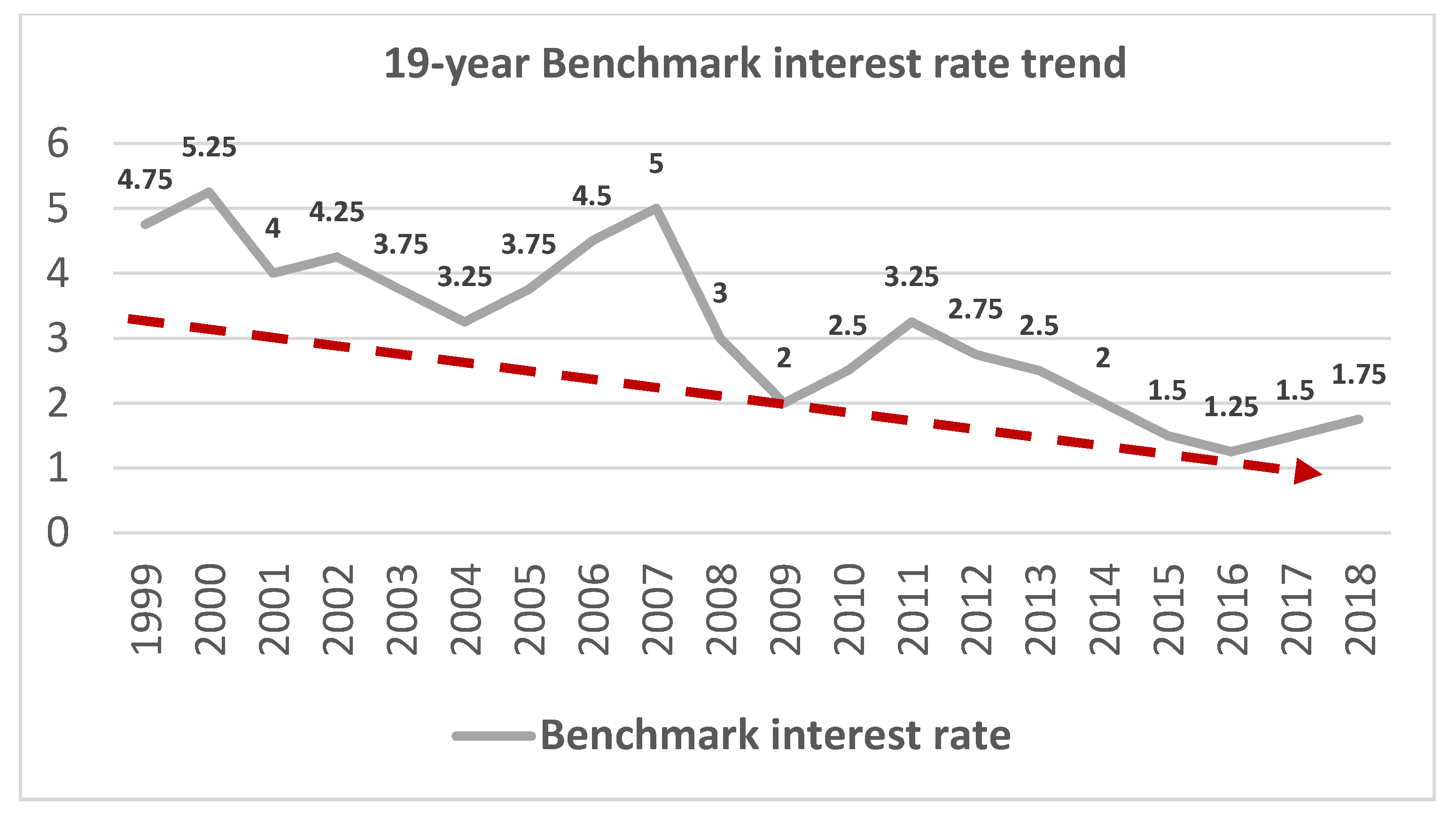
Korea’s benchmark interest rate is approximately 1.75% per annum, which is lower than that of advanced economies such as the US, where it is 2.25–2.5% [4]. For 19 years, Korea’s benchmark interest rate has declined or been frozen, as shown in Figure 1. This renders Koreans in the private sector who are not wealthy unable to collect or lend money. As a result of this low interest rate, Koreans are turning their attention to investment in stocks, which is a rather risky investment method [5]. The increased interest in stock investments is boosting research on stock price prediction. If such research can lead to suitable prediction of stock prices, the low interest rates of saving accounts can be overcome, creating opportunities for investors to easily expand their assets.

Figure 1. Nineteen-year benchmark interest rate trend.

As interest in stock investments has increased, many researchers around the world have attempted to predict future stock prices using artificial intelligence. Stock price prediction research has been historically popular, but ultimately unsatisfactory. However, as deep learning has emerged, the possibility of stock price prediction has increased. To structure stock price input data suitable for deep learning applications is fundamentally difficult. It is also difficult to construct a prediction model because of the randomness inherent in price fluctuations [6].

To predict fluctuations in stock price prediction more accurately, an in-depth analysis of input features is essential. Good performance of deep learning depends on how well the features that represent the characteristics of the whole training/test dataset are extracted. In addition, the compatibility between the input features and the target vector must be matched, which has been proven already through previous studies [7].

In this paper, we propose three models with an emphasis on input features. Previously, only simple input features, such as easy-to-use price information, were used to set input features in deep learning for stock price forecasting. However, we need to use more refined and more implicit input features to develop better prediction models. A deep learning model with good performance ultimately provides sufficient returns to users to achieve the final goal of stock price prediction. The contributions of this paper are as follows.

• We developed three stock price prediction models to determine the importance of input feature selection using input features with different characteristics. We organized models by selecting and calculating input features that are expected to be able to describe the reason for fluctuation.
• The first model uses 315 input features based on technical analysis. The second model uses 250 event binary features to represent the moment of stock price fluctuation. The third model is based on 13 existing well-known technical analysis indicators.
• The 315 input features used in Model 1 were developed as follows. After analyzing the data distribution of the 715 novel input features presented in a previous study [7], we have proposed 315 meaningful input features by eliminating all noise-prone values that affect prediction performance. This model ultimately yields profits over KOSDAQ.
• The 250 event binary input features used in Model 2 were developed as follows. We defined the moment of stock price change as an event. An event implies a turning point between the lines. If you look closely at the stock chart, you can see that the price changes depend on the relationships among the lines. Based on this, we presented 250 new event input features and developed a model that yields a higher return than the KOSPI/KODAQ. This model shows the highest performance among the three models proposed in this paper and yields the most profit.
• Finally, our stock price prediction model uses a very simple neural network structure. However, our model yielded higher profits than the Korean stock index KOSPI/KOSDAQ when using binary event features and meaningful input features. We found that event binary features and noise-prone values play a very important role in predicting stock prices.

The rest of this paper is organized as follows. Section 2 describes recent studies on stock price prediction and previous research that we have conducted. Section 3 explains the details of our proposed deep learning stock price prediction model. Section 4 provides the results of the training of each model. Section 5 describes fund simulation results using each model. Finally, Section 6 provides conclusions and topics for future studies.

2. Related Works

2.1. Recent Stock Price Prediction Studies Using Various Prediction Models

In this section, recent studies of stock price prediction using machine learning or deep learning are introduced. Stock price prediction has been attempted by many people and has received a lot of attention. In addition, the study of stock price prediction has been conducted using a wide variety of techniques. The first related study [8] used various machine learning models. Backpropagation, the long short-term memory model (LSTM), support vector machine (SVM), and other neural network models were used to predict stock price volatility with up to 68% accuracy.

The second related study [9] used stock chart images with the convolutional neural network (CNN), which showed a great amount of image sector deep learning. To predict the S&P (Standard & Poor’s) index, nine technical indicators were selected, and the performance was verified by comparing the proposed CNN model with the artificial neural network (ANN) and SVM models. The study concludes that it is appropriate to build a stock prediction model with CNN and argues that it is useful to convert time series data into graphs.

The fourth and fifth related studies [10,11] investigated the prediction of stock prices by data mining in media such as social networks or news. The authors argues that the technique used to analyze emotions in text in social media is efficient for stock price prediction. They argue that social media data is suitable for prediction because it not only implies people’s thoughts, but also accumulates in real time.

All the recent stock prediction studies [8,9,10,11] mentioned above have tested the possibility of stock price prediction using various methods. These studies [8,9,10,11] were conducted primarily by applying different deep learning models to predict stock prices. However, most studies use well-known technical indicators for input features. Our research has tested different methods that have not yet been utilized. We used a basic model for deep learning, and only the input features were changed to verify the importance of well-tuned input features and to find the types of input features that are essential for predicting stock prices.

2.2. Related Studies with Approaches Similar to Ours

In this section, we present some of the latest studies that are most similar to ours. The first related study [12] conducted a stock price prediction using multilayer perceptron (MLP) and Elman circulation network techniques. The authors verified that MLP performs better with respect to predicting changes in stock price. Therefore, we used a deep neural network based on the MLP structure.

The second study claims that the data used for learning should include characteristics of stock price fluctuations [13]. The authors explain that stock investors pay more attention to the reversal point (RP) of stock price fluctuations, instead of the stock price itself, when predicting a continuous change in stock price. After the stock has continued to rise or fall for a period of time, the sudden change in the stock price has a very decisive effect on the prediction. In this study, the authors designed the input features of the deep learning model by defining the trend reversal points, including some commonly used technical indicators. The difference from our study is that they used the LSTM model.

However, in both of these studies [12,13], we could not find a superior performance model, and there is no clear profit. The above studies have no fund simulations, and most of them have trained their model with commonly used input features. It is likely that the input features that many people commonly use in stock forecasting are meaningless because people are already investing using those indicators.

To develop a high-performance stock price prediction model, it is necessary to integrate various stock price and volume factors affecting the stock price and to supply effective learning data to the neural network through appropriate data pre-processing and filtering [14]. In this paper, we present well-tuned and calculated input features and demonstrate the performance of the newly presented input features.

2.3. Our Previous Studies on Stock Price Prediction

We have previously conducted various studies to predict stock prices using deep learning. The important point is that we used only the technical analysis features. We used novel input features that were combined and computed based on the technical analysis and advice of chart analysts. These data are different from simple price data.

The following are the previous studies we have conducted. First, we demonstrated in previous studies that using advanced input features, rather than simple price data, can achieve high predictability [7]. In addition, we found that filtering techniques for stocks with similar variation patterns yields better performance [15]. We have presented three filtering techniques, which are based on investment strategies that are often used for investment. Finally, we conducted performance evaluation of models that used different configurations of input features and target vectors. Accordingly, it has been demonstrated that the design of the deep learning model requires an appropriate combination of relevant input features and target vector.

We conducted this study based on previous studies mentioned above [7,15]. As a result, we finally derive stock price prediction models that show a better profit than the domestic stock price index KOSPI/KOSDAQ.

3. Design and Development of the Stock Price Prediction Model

In this section, we present three stock price prediction models. This section is organized as follows. Section 3.1 describes the learning model structure. Section 3.2 explains the newly proposed Model 1 by refining further the features mentioned as novel input features in previous research. Section 3.3 describes Model 2 with the new event features, which we called binary features. Section 3.4 explains Model 3, which only consists of existing well-known technical indicators. Section 3.5 discusses the target vector of the prediction model in detail. Finally, Section 3.6 discusses the preprocessing and normalization methods.

3.1. Deep Neural Network (DNN)

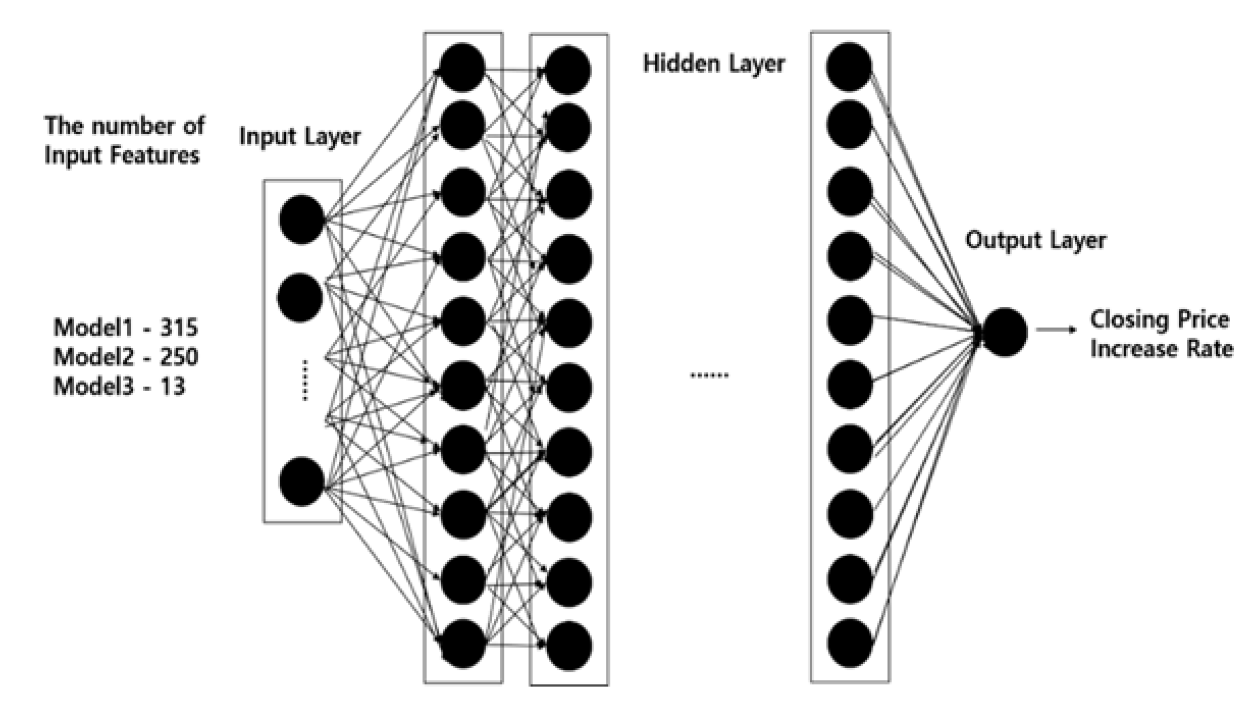
We used a deep neural network (DNN) to develop a model for stock price prediction. A DNN is a type of feedforward neural network composed of input, hidden, and output layers. Each node, except for the input layer, consists of neurons, which use nonlinear activation functions [16]. We use the backpropagation method for training. The backpropagation method is a process of modifying the parameters by making the difference between the predicted value and the correct answer small [17]. The structure of the three models proposed in this study is the same as that of the DNN, as shown in Figure 2. The input layer of the DNN consists of 315, 250, and 13 nodes according to the number of input features in each model. The DNN has 250 hidden layers. The output layer consists of one node and predicts the closing price after 6 days, which is explained further in Section 3.5.

Figure 2. Deep neural network structure used in our study.

We use the mean square error (MSE) method to calculate the difference between the predicted value and the correct answer. Equation (1) represents the MSE error calculation formula. MSE is a method of averaging the difference of each value by squaring. The error is squared, therefore larger differences reflect greater error [18]. $\widehat{y_i}$ represents the predicted value derived from the neural network result, and $y_i$ is the correct answer to predict. The difference between these values is squared and added together, and the value divided by the number of data is the MSE value.

$$\mathrm{Mean}\mathrm{Squared}\mathrm{Error}=\frac{1}{n}{{\displaystyle \sum }}_i{\left(\widehat{y_i}-y_i\right)}^2$$

(1)

We use the mean absolute error (MAE) to estimate the training error of each model accurately. This value averages the absolute value of the error between each predicted value and the correct answer [19]. The MAE is the simplest regression error metric. Equation (2) represents the MAE error calculation formula.

$$\mathrm{Mean}\mathrm{Absolute}\mathrm{Error}=\frac{1}{\mathrm{n}}{{\displaystyle \sum }}_{\mathrm{i}}\left|\widehat{{\mathrm{y}}_{\mathrm{i}}}-{\mathrm{y}}_{\mathrm{i}}\right|.$$

(2)

Later, to find the best model, we use the measured error values to compare the performance of the three models.

3.2. Model 1: 315 Novel Input Features Model

Model 1 is the next version of a stock price prediction model using 715 novel input features presented in a previous study [7]. A total of 715 input features were presented according to our own technical analysis and opinions of other stock chart analysts. Table 1 is a brief description of the configuration of the 715 input features [7]. A previous model using these 715 features was able to make a profit. However, we determined that there are excessive duplicate meaningful input features. In addition, there are some possibilities to improve performance through feature value preprocessing and normalization. We refined these 715 feature values and removed less meaningful features to improve the performance of the prediction model.

Table 1. Novel input features presented in previous studies.

Description of 715 Features	Number of Features
1. Gradient of moving average line	10
2. Sum of long-term moving average gradient	2
3. Gradient of 5-days/20-days volume moving average	3
4. Change in volume moving average	60
5. Difference between yesterday’s and today’s moving average	40
6. The change of long and short-term moving average and the point of golden/dead cross	220
7. The change of long and short-term volume moving average and the point of golden/dead cross	140
8. Disparity of moving average	10
9. Disparity of 60-days/120-days volume moving average	30
10. Disparity of 20-days/60-days volume moving average	30
11. Disparity of 5-days/20-days volume moving average	30
12. Change in closing price on a specific day	110
13. Other simple price indicators	30

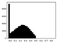
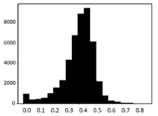
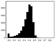
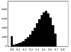
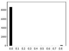
The process of feature refinement is as follows. First, distributions of each of the 715 features were calculated in the form of a histogram to determine the value distributions. We found that there are some noisy features that are either biased or single-valued. These data are likely to interfere with training performance.

An example of the data distribution is shown in Table 2. Valid values mostly show Gaussian distributions. Outliers are sparse among these data, and there are also some biased data. However, they can be cleared by the data normalization algorithm that will be discussed in Section 3.6. The histograms presented at the bottom of Table 2 show examples of heavily biased, even single-valued, features. These features should be eliminated because they definitely have no significant effect on performance improvement. Through this feature refinement process, we reduced the number of features from 715 to 315.

Table 2. Histogram of data distribution of input features.

	Histogram of Data Distribution
Valid Distribution of Feature Values
Invalid Distribution of Feature Values

Table 3 shows details of the input features of Model 1. It has a total 315 input features. Here, moving average refers to the average stock price. The moving average of the closing price is denoted as $MA$, while the moving average of volume is expressed as $VMA$. For example, the closing price of a stock at trading date t is expressed as $Clos{e}_t^s$ whereas the moving average of the closing price over five days can be expressed as $MA{5}_t^s$. Equations (3) and (4) show examples of 5-day moving averages of the closing price and volume [20].

$$MA{5}_t^s=\frac{1}{5}{\displaystyle \sum }_{k=0}^{4}Clos{e}_{t-k}^s$$

(3)

$$\mathrm{VMA}{5}_{\mathrm{t}}^{\mathrm{s}}=\frac{1}{5}{{\displaystyle \sum }}_{k=0}^4{\mathrm{Volume}}_{\mathrm{t}-k}^{\mathrm{s}}.$$

(4)

Table 3. Description of 315 input features for Model 1.

Feature Descriptions	Formula	Number of Features
Gradient of the moving average/volume moving average of k trading day	$Grad{k}_t^s=\frac{MA{k}_t^s-MA{k}_{t-1}^s}{MA{k}_t^s}x100 \left(k=5,10,20,60,120\right)$ $VGrad{k}_t^s=\frac{VMA{k}_t^s-VMA{k}_{t-1}^s}{VMA{k}_t^s}x100 \left(k=5,10,20\right)$	13
Sum of gradient of 60 and 120 days during past 40 days	$SumGk={\displaystyle {\displaystyle \sum }_{n=0}^{39}}Grad{k}_t^s\left(k=60,120\right)$	2
Rate of change of volume moving average of the k days	$RoCVM{A}_t^s=\frac{VMA{k}_t^s}{VMA{k}_{t-j}^s} \left(k=60,120\right)$ $( j=1,2,3,4,5,7,9,11,13,15,18,21,24,27,30,34,38,$ $42,46,50,55,60,65,70,75,80,85,90,95)$	60
Rate of change of closing price	$Ro{C}_t^s= \frac{Clos{e}_t^s-Clos{e}_{t-j}^s}{Clos{e}_t^s}$ $(j=1,2,3,4,5,6,7,8,9,10,11,12,13,14,15,16,17,18,19,20,22,24,26,28$ $,30,32,34,36,38,40,42,44,46,48,50,52,54,56,58,60,63,66,69,$ $72,75,78,81,84,87,90,94,98,102,106,110,114,120)$	110
Disparity from moving average of k days	$Disp{k}_t^s= \frac{Clos{e}_t^s-MA{k}_{t-j}^s}{Clos{e}_t^s}$ $\left(k=5,10,20,60,120, j=0,1\right)$	10
Disparity of k days and n days’ volume moving average	$VDispk\_n_t^s= \frac{VMA{k}_{t-j}^s}{VMA{n}_{t-j}^s}$ $\left(k,n\right)=\left(0,5\right),\left(60,120\right),\left(5,20\right), \left(20,60\right)$ $(j=1,2,3,4,5,7,9,11,13,15,18,21,24,27,30,34,38,$ $42,46,50,55,60,65,70,75,80,85,90,95)$	120

Based on the above equations, we describe 315 input features. First, we calculated the gradients of the $MA$s and the $VMA$s. This produces 13 input features. The second is the feature using the gradient of the 60-day and 120-day $MA$. The sum of the gradient of the two $MA$s for 40 days constitutes two input features. The third is the rate of change of the $VMA$. This ratio is calculated based on a specific j -day and the moving average line of 60 days and 120 days. The fourth input features concern changes in the closing prices. It is also calculated on a specific j-day basis and adds 110 features. The fifth is disparity features, which denotes how close the closing price is from the $MA$. We use yesterday and today’s disparity and create 10 input features. Sixth, the disparity of the k-days $VMA$s and the n-days $VMA$s were calculated. They were calculated based on a specific j-day and led to 120 more input features.

3.3. Model 2: Event Binary Features Model

The second model we have proposed uses event binary features. Stock chart analysts observe charts and capture price fluctuation events. For example, the intersection of the moving average lines and the point of receiving the support and resistance are considered to be very important. In addition to the chart analysts, many people consider these points as an event and make decisions to buy or sell stocks. Indeed, many studies have shown statistically and numerically that this is the starting point for price increases or decreases. In this paper, these points are represented as binary values and used as features. The characteristic of binary data is that although the value is simple, it has an event in reality. Therefore, we anticipate that using this data will be very effective for improving performance. Model 2 consists of the event binary feature and the price feature, with a total of 250 features. The detailed configuration is shown in Table 4 and Table 5.

Table 4. Detail of price features.

Price Feature Description	Formula	Number of Features
Gradient of the moving average of k trading days	${\mathrm{Gradk}}_{\mathrm{t}}^{\mathrm{s}}=\frac{{\mathrm{MAk}}_{\mathrm{t}}^{\mathrm{s}}-{\mathrm{MAk}}_{\mathrm{t}-1}^{\mathrm{s}}}{{\mathrm{MAk}}_{\mathrm{t}}^{\mathrm{s}}}\mathrm{x}100$, $\left(\mathrm{k}=5,10,20,60,120\right)$	5
Sum of gradient of 10 trading days during past i days	${\displaystyle \sum }_{\mathrm{n}=0}^{\mathrm{i}}\mathrm{Grad}{10}_{\mathrm{t}}^{\mathrm{s}}$, $\left(\mathrm{i}=5,10\right)$	2
Sum of gradient of 20 trading days during past i days	${\displaystyle \sum }_{\mathrm{n}=0}^{\mathrm{i}}\mathrm{Grad}{20}_{\mathrm{t}}^{\mathrm{s}}$, $\left(\mathrm{i}=10,20,40\right)$	3
Sum of gradient of 60 trading days during past i days	${\displaystyle \sum }_{\mathrm{n}=0}^{\mathrm{i}}\mathrm{Grad}{60}_{\mathrm{t}}^{\mathrm{s}}$, $\left(\mathrm{i}=10,20,40,80\right)$	4
Sum of gradient of 120 trading days during past i days	${\displaystyle \sum }_{\mathrm{n}=0}^{\mathrm{i}}\mathrm{Grad}{120}_{\mathrm{t}}^{\mathrm{s}}$, $\left(\mathrm{i}=20,40,80\right)$	3
Rate of change of closing price in a specific j days.	${\mathrm{RoC}}_{\mathrm{t}}^{\mathrm{s}}=\frac{{\mathrm{Close}}_{\mathrm{t}}^{\mathrm{s}}-{\mathrm{Close}}_{\mathrm{t}-\mathrm{j}}^{\mathrm{s}}}{{\mathrm{Close}}_{\mathrm{t}}^{\mathrm{s}}}\left(\mathrm{j}=1,2,4,7,12,20,33,54,88,133\right)$	1
Gradient of the volume moving average of 5 trading days	$\mathrm{VGrad}{5}_{\mathrm{t}}^{\mathrm{s}}=\frac{\mathrm{MA}{5}_{\mathrm{t}}^{\mathrm{s}}-\mathrm{MA}{5}_{\mathrm{t}-1}^{\mathrm{s}}}{\mathrm{MA}{5}_{\mathrm{t}}^{\mathrm{s}}}\times 100$	1
Disparity of the volume moving average of k trading days	${\mathrm{VDispk}}_{\mathrm{t}}^{\mathrm{s}}=\frac{{\mathrm{Volume}}_{\mathrm{t}}^{\mathrm{s}}-{\mathrm{VMAk}}_{\mathrm{t}}^{\mathrm{s}}}{{\mathrm{Volume}}_{\mathrm{t}}^{\mathrm{s}}},\left(\mathrm{k}=5,20,60,120\right)$	4
Rate of 120 day volume moving average and j days ago volume moving average	$\mathrm{VMA}{60}_{\mathrm{sc}}=\frac{\mathrm{VMA}{60}_{\mathrm{t}}^{\mathrm{s}}}{\mathrm{VMA}{60}_{\mathrm{t}-\mathrm{j}}^{\mathrm{s}}},\left(\mathrm{j}=20,60,120\right)$	3
Rate of 120 day volume moving average and j days ago volume moving average	$\mathrm{VMA}{120}_{\mathrm{sc}}=\frac{\mathrm{VMA}{120}_{\mathrm{t}}^{\mathrm{s}}}{\mathrm{VMA}{120}_{\mathrm{t}-\mathrm{j}}^{\mathrm{s}}},\left(\mathrm{j}=10,20,60,120\right)$	4
Disparity from MA of k days of stock price	${\mathrm{Dispk}}_{\mathrm{t}}^{\mathrm{s}}=\frac{{\mathrm{Close}}_{\mathrm{t}}^{\mathrm{s}}-{\mathrm{MAk}}_{\mathrm{t}}^{\mathrm{s}}}{{\mathrm{Close}}_{\mathrm{t}}^{\mathrm{s}}},\left(\mathrm{k}=5,10,20,60,120\right)$	5
Rate of change of volume in today and yesterday	${\mathrm{RoV}}_{\mathrm{t}}^{\mathrm{s}}=\frac{{\mathrm{Volume}}_{\mathrm{t}-\mathrm{i}}^{\mathrm{s}}-{\mathrm{Volume}}_{\mathrm{t}-\mathrm{i}-1}^{\mathrm{s}}}{{\mathrm{Volume}}_{\mathrm{t}}^{\mathrm{s}}},\left(\mathrm{i}=0,1\right)$	2

Table 5. Detail of event binary features.

Binary Features Description	Formula	Number of Features
Turn up/down point between moving average lines	$\{\begin{array}{c}true\left(=1\right) Grad{k}_{t-1}^s<0 and Grad{k}_t^s\ge 0 \\ false\left(=-1\right) Otherwise\end{array}, \left(k=5,10,20\right)$	30
Golden cross point between moving average lines	$\{\begin{array}{c}true\left(=1\right) MA{5}_t^s< MA{k}_t^s and MA{5}_t^s\ge MA{k}_t^s \\ false\left(=-1\right) Otherwise\end{array}, \left(k=10,20,60,120\right)$	45
	$\{\begin{array}{c}true\left(=1\right) MA{10}_t^s< MA{k}_t^s and MA{10}_t^s\ge MA{k}_t^s \\ false\left(=-1\right) Otherwise\end{array},\left(k=20,60,120\right)$
	$\{\begin{array}{c}true\left(=1\right) MA{20}_t^s< MA{k}_t^s and MA{20}_t^s\ge MA{k}_t^s \\ false\left(=-1\right) Otherwise\end{array},\left(k=60,120\right)$
Dead cross point between moving average lines	$\{\begin{array}{c}true\left(=1\right) MA{5}_t^s> MA{k}_t^s and MA{5}_t^s\le MA{k}_t^s \\ false\left(=-1\right) Otherwise\end{array}, \left(k=10,20,60,120\right)$	45
	$\{\begin{array}{c}true\left(=1\right) MA{10}_t^s> MA{k}_t^s and MA{10}_t^s\le MA{k}_t^s \\ false\left(=-1\right) Otherwise\end{array}$, $\left(k=20,60,120\right)$
	$\{\begin{array}{c}true\left(=1\right) MA{20}_t^s> MA{k}_t^s and MA{20}_t^s\le MA{k}_t^s \\ false\left(=-1\right) Otherwise\end{array},\left(k=60,120\right)$
Support and resist point for moving average lines	$If Ope{n}_t^s>Clos{e}_t^s$ $\{\begin{array}{c} true if(MA{k}_t^s> Clos{e}_t^s and MA{k}_t^s< Hig{h}_t^s)\\ \\ false otherwise\end{array}$ $Else$ $\{\begin{array}{c} true if(MA{k}_t^s> Ope{n}_t^s and MA{k}_t^s< Hih{g}_t^s) \\ \\ false otherwise\end{array}, \left(k=5,10,20\right)$	12
Upward/downward penetration point between moving average lines	$If Ope{n}_t^s>Clos{e}_t^s$ $\{\begin{array}{c} true if(MA{k}_t^s> Lo{w}_t^s and MA{k}_t^s< Clos{e}_t^s) \\ \\ false otherwise\end{array}$ $Else$ $\{\begin{array}{c} true if(MA{k}_t^s> Lo{w}_t^s and MA{k}_t^s< Ope{n}_t^s) \\ \\ false otherwise\end{array}, \left(k=5,10,20\right)$	12
Golden cross point between volume moving average lines	$\{\begin{array}{c}true\left(=1\right) VMA{5}_t^s< VMA{k}_t^s and VMA{5}_t^s\ge VMA{k}_t^s \\ false\left(=-1\right) Otherwise\end{array},\left(k=20,60,120\right)$	25
	$\{\begin{array}{c}true\left(=1\right) VMA{20}_t^s< VMA{k}_t^s and VMA{20}_t^s\ge VMA{k}_t^s \\ false\left(=-1\right) Otherwise\end{array},\left(k=60,120\right)$
Dead cross point between volume moving average lines	$\{\begin{array}{c}true\left(=1\right) VMA{5}_t^s> VMA{k}_t^s and VMA{5}_t^s\le VMA{k}_t^s \\ false\left(=-1\right) Otherwise\end{array},\left(k=20,60,120\right)$	25
	$\{\begin{array}{c}true\left(=1\right) VMA{20}_t^s> VMA{k}_t^s and VMA{20}_t^s\le VMA{k}_t^s \\ false\left(=-1\right) Otherwise\end{array},\left(k=20,60,120\right)$
Relationship of volume moving average lines arrangement	$\{\begin{array}{c}true\left(=1\right) VMA{5}_t^s\ge VMA{k}_t^s \\ false\left(=-1\right) Otherwise\end{array},\left(k=20,60,120\right)$	6
	$\{\begin{array}{c}true\left(=1\right) VMA{20}_t^s\ge VMA{k}_t^s \\ false\left(=-1\right) Otherwise\end{array},\left(k=60,120\right)$
	$\{\begin{array}{c}true\left(=1\right) VMA{60}_t^s\ge VMA{k}_t^s \\ false\left(=-1\right) Otherwise\end{array},\left(k=120\right)$
Relationship between volume moving average of 5 trading days and volume moving average of k trading days	$\{\begin{array}{c}true\left(=1\right) VMA{5}_t^s\ge VMA{k}_t^s\\ false\left(=-1\right) Otherwise\end{array},\left(k=5,20,60,120\right)$	4

There are 46 price features used with binary features in Table 4. These consist of $MA$s, the gradient of $MA$s, the gradient of $VMA$s, and disparity. Each $MA$ and $VMA$ and the disparity, are calculated at intervals of 5/10/20/60/120 days.

The configuration of the event binary features is shown in Table 5 (continued on the next page). There are 30 turn-up or down features, which means the phase at which the slope of $MA$ becomes negative or positive. There are 90 features related to the golden or dead cross point of the $MA$. There are 12 support- or resist-related features and 12 features related to the upward or downward penetration point of $MA$. Binary features related to volume consist of 50 golden or dead cross points, 6 relationships between $VMA$s, and lastly, 4 relationships between volume and $VMA$s. In total, 204 binary features were created.

3.4. Model 3: Existing Well-Known Technical Analysis Indicator Model

Finally, the third model uses some well-known technical analysis indicators as input features. A total of 13 input features are common indicators that can be obtained from any home trading system software. We attempted to verify the actual prediction performance of the technical indicators that are publicly available. We expected that commonly used indicators would be less predictable because people use it a lot as it is a well-known investment indicator. Therefore, we performed an experiment to prove this scientifically.

The first indicator we used is the relative strength index (RSI). This indicator represents the relative strength of the price increase and decline. This indicator measures the average value of the change between today’s and yesterday’s price over a period of time. If the amount of change that has risen is large, it can be categorized as over-buying. If the situation is the opposite, it can be categorized as over-selling. The RSI formula is shown in Equation (5). If today’s closing price is higher than the previous day’s closing price, then it is added to the ups (U). If it falls, it is added to the downs (D). Then, the U and D values are obtained for a certain period of time, after which the averages of U and D are calculated. At this time, the average of U values is called AU (average ups), and the average of D values is called AD (average downs). The ratio of AU to AD is called the relative strength (RS). A large value of RS means that the increase range is larger than the decrease range for a certain period [21]. We calculated the period of RSI based on 14 days and constructed two input indicators. One of the two indicators is the RSI value, and the other is the buying or selling position. When the value is 70 or more, the selling position is set to 0, and when the value is 30 or less, the buying position is set to 1. When the value is 30 or more and 70 or less, the values are set to 0.5.

$$RSI=\frac{AU}{AU+AD}.$$

(5)

The second indicator we used is the stochastic indicator, which shows the position of the closing price as a percentage of the oscillation of the stock price over a certain period [22]. This value represents the position of the current price within the range between the highest price and the lowest price for the most recent n days. The value increases when the buying power is stronger than the selling power, and the value decreases when the selling power is stronger than the buying power. This indicator reflects the properties of the stock price fluctuation, consisting of %K, which is the main value, and %D, which is the moving average of %K. If %K falls below 20% and then rises again, it can be considered a buying signal. If it rises above 80% and then drops again, it is a selling signal. Therefore, the index consists of three indicators, i.e., %K, %D, and a trading binary indicator. The calculation formula for %K and %D is shown in Equation (6).

$Clos{e}_t^s$ represents the closing price of stock s on day t, $MinPric{e}_n^s$ is the value when the price of stock s is the smallest in the last n days, and $MaxPric{e}_n^s$ is the value when the price of stock s is the highest in the last n days. The %D value is the m days exponential moving average of the %K value [23].

$$\mathit{Stochastic}\left(\%K_t^s, \%D_t^s\right)=(\frac{Clos{e}_t^s-MinPric{e}_n^s}{MaxPric{e}_{10}^s+MinPric{e}_n^s}, EMA\left(\%K, m\right))$$

(6)

where $MinPric{e}_t^s$ = The minimum price of the last t-day stocks, $MaxPric{e}_t^s=Themaximumpriceofthelastt-daystocksEP=\frac{2}{period+1}$ $EMA\left(value,period\left(t\right)\right)=value\ast EP+EM{A}_{t-1}\ast \left(1-EP\right)$.

The third indicator is the commodity channel index (CCI) indicator [24]. CCI is a measure of the deviation between the average stock price and typical stock price. The CCI is a momentum-based oscillator used to help investors determine when an investment vehicle is reaching a condition of being overbought or oversold. CCI is sometimes used to find reversals and variances. A high CCI means that the current stock price is higher than the average stock price, and a low CCI means that the current stock price is lower than the average stock price. Based on this, we define CCI values and a trading binary indicator as two features. If CCI is positive, it is recognized as a strong signal and regarded as a buying point. If CCI is negative, it is recognized as a weak signal and regarded as a selling point. The calculation formula for CCI is given in Equation (7).

$$CCI=\frac{Typical Price-MA}{0.015 \times Mean Deviation}$$

(7)

where $TypicalPrice={\displaystyle \sum }_{i=1}^P\frac{Clos{e}_t^s+Hig{h}_t^s+Lo{w}_t^s}{3}$, $P=Numberofperiods$, $MA=\frac{\left({{\displaystyle \sum }}_{i=1}^{P}TypicalPrice\right)}{P}$, $MeanDeviation=\frac{\left({{\displaystyle \sum }}_{i=1}^P|TypicalPrice-MA|\right)}{P}$.

Next, a Bollinger band is defined by a set of lines plotted two standard deviations away from the moving average of stock price [25]. The Bollinger bands are made up of three bands in relation to price. The center band is typically the simple moving average. The equation for the three bands is shown in Equation (8). The middle band (MB) is the moving average value of the closing price for 20 days. By using this value to obtain the standard deviation, multiplying the value by 2, and calculating it with the MB value, upper band (UB) and lower band (LB) values are derived. This indicator creates a total of four features, i.e., the upper Bollinger band, Bollinger band, lower Bollinger band, and a trading binary signal. When the stock price movement is high, the breadth of the band is widened, and when the movement is low, the breadth of the band is narrowed [26].

$$\begin{gathered} MB\left(Middle Band\right)=\frac{1}{20}{\displaystyle \sum }_{k=0}^{19}Clos{e}_{t-k}^s \\ UB\left(Upper Band\right)=MB+ sqrt\left(pow\left( Clos{e}_t^s-MB\right)\right)\ast 2 \\ LB\left(Lower Band\right)=MB- sqrt\left(pow\left( Clos{e}_t^s-MB\right)\right)\ast 2 \end{gathered}$$

(8)

The last technical indicator is the Volume ROC. This value indicates the difference between today’s volume and the trading volume n days ago [27], which represents the rate of change in volume. If this value increases sharply, it denotes the price break out point. The formula is as shown in Equation (9).

$$Volume ROC= \frac{Volum{e}_t^s- Volum{e}_{t-n}^s}{Volum{e}_{t-n}^s}\ast 100$$

(9)

3.5. Target Vector

This section describes the target vector configuration. We designed the target vector based on reinforcement learning theory. Reinforcement learning is a machine learning technique concerned with how software agents ought to take action so as to maximize cumulative reward [28]. The optimal policy decision is made through reward, and learning progresses to maximize reward. In reinforcement learning, this is called “expected cumulative future discounted reward. “Expected” mentions the anticipated value. “Cumulative” means the summation. “Future” means the fact that it is an anticipated value of a future amount with respect to the present amount. “Discounted” means the gamma factor, which is a way to adjust the importance of how much we value rewards at future time steps. “Reward” means the main amount of attention received from the environment [29]. The formula for expected cumulative future discounted reward is shown in Equation (10).

$$Expected cumulative future discounted reward=G_t=E[{\displaystyle \sum }_{j=1}^{\infty }{\gamma }^{j-1}{R}_{t+j}]$$

(10)

We wished to predict the increase rate of closing price after 6 days. When calculating the increase rate, it is necessary to reflect more recent change rates in the closing price than older ones because they can better reflect the direction of the latest stock price. Therefore, we calculated the target based on expected cumulative future discounted reward. The formula for our target is shown in Equation (11).

$$Target value =\frac{{{\displaystyle \sum }}_{t=0}^6{\beta }^{t+1}\ast \frac{Close pric{e}_{t+1}^s}{Close pric{e}_t^s}}{\theta }$$

(11)

where $\beta =$ Coefficient of ratio reflecting closing price, $\theta =$ rate of increase or decrease in closing price.

We have targeted whether the closing price has risen by more than 13% compared with 6 days ago. Therefore, we set $\theta$ = 13. $\beta$ is a ratio that reflects the daily closing price. If $\beta$ is 0.5, we consider it to be a reasonable constant for estimating the short term (today or tomorrow). Therefore, we set it to 0.81, as we wanted to predict 6 days.

3.6. Feature Normalization

This part of Section 3 concerns feature value normalization. When processing large amounts of data, data normalization is essential. Theoretically, using a deep learning model structure such as a deep neural network or multilayer perceptron does not require normalization or standardization of the input features. However, data normalization has the following advantages. First, the training speed is improved. We use stock data from 2000 to 2019, and with more than 3000 stocks, there is a very large amount of data. Second, normalization helps to avoid falling into local optima during training. For these reasons, we performed data normalization before feeding them into the deep learning model [30]. We used the normalizing technique to linearize the feature values. This method linearly maps the original values to the new values found by the assigned min to max value [31]. The value we want to obtain is $\widetilde{x_i}$ which is calculated from the minimum and maximum values of the data. $mi{n}_i$ is the original minimum value, and $ma{x}_i$ is the original maximum value. The new minimum value is $lo{w}_i$, and the new maximum value is $hig{h}_i$. Equation (12) shows the formula for our normalization technique. Using Equation (12), all of the input features used in Models 1, 2, and 3 are normalized to the range (−1,1).

$$\widetilde{x_i}=lo{w}_i+\frac{hig{h}_i- lo{w}_i}{ma{x}_i-mi{n}_i}\ast \left(x_i- mi{n}_i\right)$$

(12)

4. Experimental Results

We implemented a deep learning model using Tensorflow and Keras and found that the errors decreased during the test process. The configuration of the model is shown in Table 6, and the parameters of all three models are set to be identical. Models 1, 2, and 3 use different input features, as described before. We expected that the proper combination and calculation of input features would lead to different performances for each model.

Table 6. Results of training of prediction model.

	Model 1	Model 2	Model 3
Number of Input Features	315	250	13
Configuration of Input Features	Novel input feature using price information	Simple price feature + Binary chart feature	Only technical indicator
Activation Function	Tahn	Tahn	Tahn
Dropout	0.5	0.5	0.5
Optimizer	RMSprop	RMSprop	RMSprop
MSE	0.1105	0.0795	0.1171
MAE	0.2447	0.2162	0.2498
Fund Simulation	O	O	X

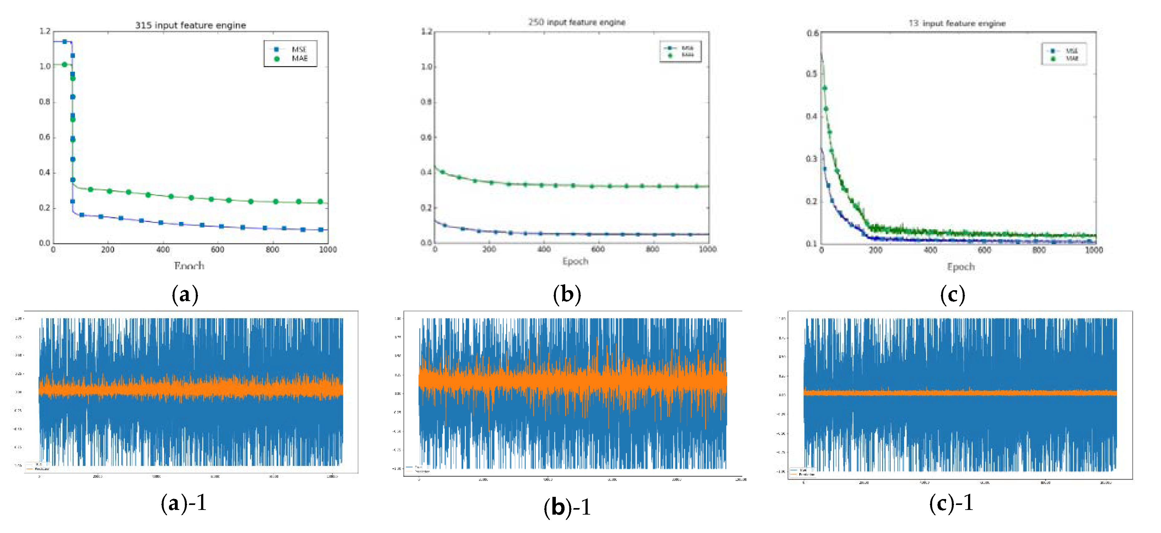
As a result of test, the MSE of Model 1 decreased to 0.1105, and the MAE of Model 1 decreased to 0.2447. In Model 2, the MSE decreased to 0.0795 and the MAE decreased to 0.2162. In Model 3, the MSE decreased to 0.1171 and the MAE decreased to 0.2498. In summary, Model 2 has the best performance with respect to MSE and MAE. The results of the following experiments can be found in Figure 3.

Figure 3. These (a–c) figures are mean square error (MSE) and mean absolute error (MAE) graph of Model 1, 2, 3 using test data. (a)-1 is the prediction result graph of Model 1, (b)-1 is Model 2, and (c)-1 is Model 3, respectively.

The results of the following experiments can be found in Figure 3a–c. Each of the three models presented can be characterized as follows. In the case of Model 1 in Figure 3a, the error was very high at the beginning, but it decreased as progressed. In Model 2 in Figure 3b, the error was low from the beginning. We conclude that because it is composed of binary features, the noise is low, and the prediction performance is good from the beginning. In the case of Model 3, data used as input features were publicly used by investors. In Figure 3c, the error was reduced, but the noise was very high.

All three models used Tahn as an activation function and the RMSprop optimization technique. The dropout ratio was set to 0.5. The data used for these experiments consisted of the data from the period from 2000 to September 2019. To further compare the performance and accuracy of each model, we added predicted result graphs to Figure 3(a)-1,(b)-1,(c)-1. We also used test data for these graphs. The blue graph is the actual value and the orange graph is the prediction value. According to these graphs, we can see the best performance of Model 2.

Table 7 compares the MSE and MAE of the three models. Model 2 showed the best values, which were −38.99 and −47.29 compared with Models 1 and 3 respectively. In addition, Model 1 showed better performance than Model 3 by approximately −5.97 [32,33]. Finally, the performance of Model 3 was the worst, and even there are no recommended stocks to conduct fund simulations, we can say from this result that Model 3 is an inappropriate model to use for stock price prediction based on deep learning.

Table 7. Performance comparison of three models.

Forecasting Model	MSE	MAE	Comparison of Prediction Accuracy with Model 1% (MSE)	Comparison of Prediction Accuracy with Model 2% (MSE)	Comparison of Prediction Accuracy with Model 3% (MSE)
Model 1	0.1105	0.2447	X	28.05	−5.97
Model 2	0.0795	0.2162	−38.99	X	−47.29
Model 3	0.1171	0.2498	5.63	32.10	X

5. Performance Evaluation through Fund Simulation

We conducted fund simulations to measure the cumulative investment profits of each model. To set up a precise fund-simulation environment, we set up the fund simulation using a period that is different from the training and test data periods. We conducted fund simulations using data from September 2015 to November 2019. In addition, we used a previously developed fund simulation system [34] that can find the best trading policy for a set of recommended stocks.

When fund simulation is conducted, validation data is applied to the prediction model to obtain recommendations for every date and every stock symbol. In addition, ach prediction result has an additional probability field for the prediction. We call this a “$predictionvalue$”, and this value is estimated between 0 and 1. We set a certain threshold $\theta$, to exclude too low $predictionvalue$. If the $predictionvalue$ is too low, the number of stock trading will increase, while the profit per trade decrease in fund simulation. Therefore, fund simulation is performed only when it is above a certain threshold. When the prediction model defined by the parameter $w$ is $f$ and the input expression of the stock for $f$ on a specific date $t$ is $s_t$, the equation for the $predictionvalue$ value is as follows. We set $\theta$ above 0.1 in the fund simulation.

$$prediction value=f\left(s_t;w\right)\ge \theta$$

(13)

Our fund simulation program combines various policies based on recommended items and dates. Then it calculates the profit and hit rate to get the best trading policy. The Trade Policy generated by the Fund Simulation Program consists of a total of eight fields. The first factor is the “Buy discount rate”, which is the percentage of purchase price compared to the previous day’s close price at buying the recommended stocks. Second is “Target profit rate”. This factor represents the target rate of profit that we set at buying stocks. Third factor is “Stop-loss rate”. Stop-loss rate is the loss rate when the purchased stocks should be loss-cut. If the stop-loss rate is −12%, it will be sold automatically if the current price is −12% lower than the buying price. Fourth, “Profit rate” is the ratio of the actual profit. Fifth the “Maximum holding period” is the maximum number of days to hold the purchased stock. For example, if the maximum holding date is 5, and the stock price does not reach the target profit rate or stop-loss rate for five days after the purchase date, it will be automatically sold at the closing price of the final date. Sixth, “Profit rate per trade” means the ratio of the profit that can be obtained in one trading of the whole trading. “Profit rate per daily trade” is a daily calculation of “Profit rate per trade”. Finally, “Hit ratio” refers to the percentage of stocks that were sold at the target profit price. We conducted the fund simulation using only the results with a predictor value of 0.1 or higher for each model, and the result of optimal trading policy is as shown in Table 8

Table 8. Optimal trading strategy for each model.

Optimal Trading Policy for Each Model
	Buy Discount Rate (%)	Target Profit Rate (%)	Stop-Loss Rate (%)	Profit Rate (%)	Maximum Holding Period (Day)	Profit Rate per Trade (%)	Profit Rate per Daily Trade (%)	Hit Ratio (%)
Model 1	+0	+24	−12	52.6	22	1.86	0.11	27.3
Model 2	−6	+22	−12	68.5	21	7.61	0.46	38.2
Model 3	X	X	X	X	X	X	X	X

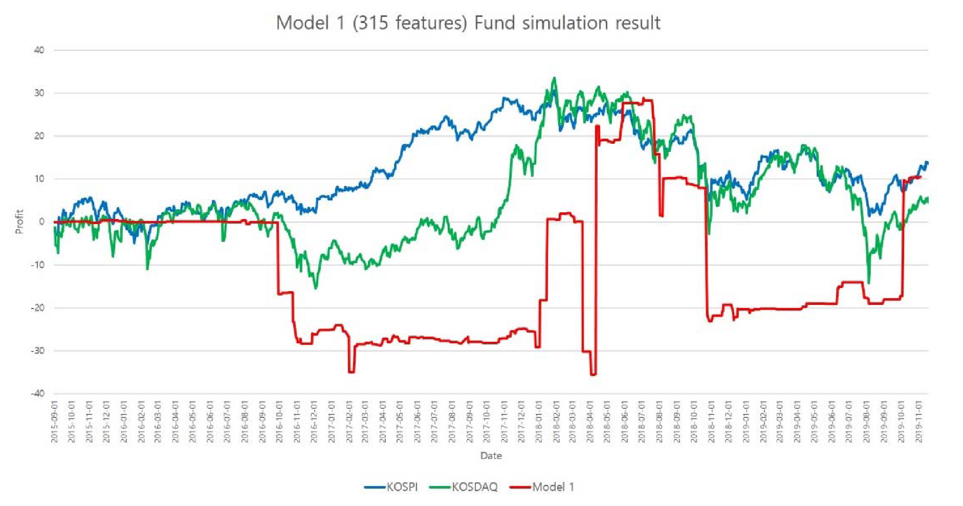
Model 1 purchases stock as the same price as the previous day’s close price because the “buy discount rate” is +0. According to fund simulation, we can get the best profit when we sell stock that reach at +24% profit or −12% loss for up to 22 days. As a result, Model 1 was able to get 52.6% profit of the investment, and the hit ratio was 27.3%. For Model 2, it was best way to purchase stock at −6% lower than the previous day. We can get the best profit when we sell stock that reach at +22% profit or −12% loss for up to 21 days. As a result, Model 2 was able to get 68.5% profit of the investment, and the hit ratio was 38.2%. The average profit of model was 7.61% per trading. In the case of Model 3, there are no results in Table 8 because the predictor value is so low that fund simulation could not be performed.

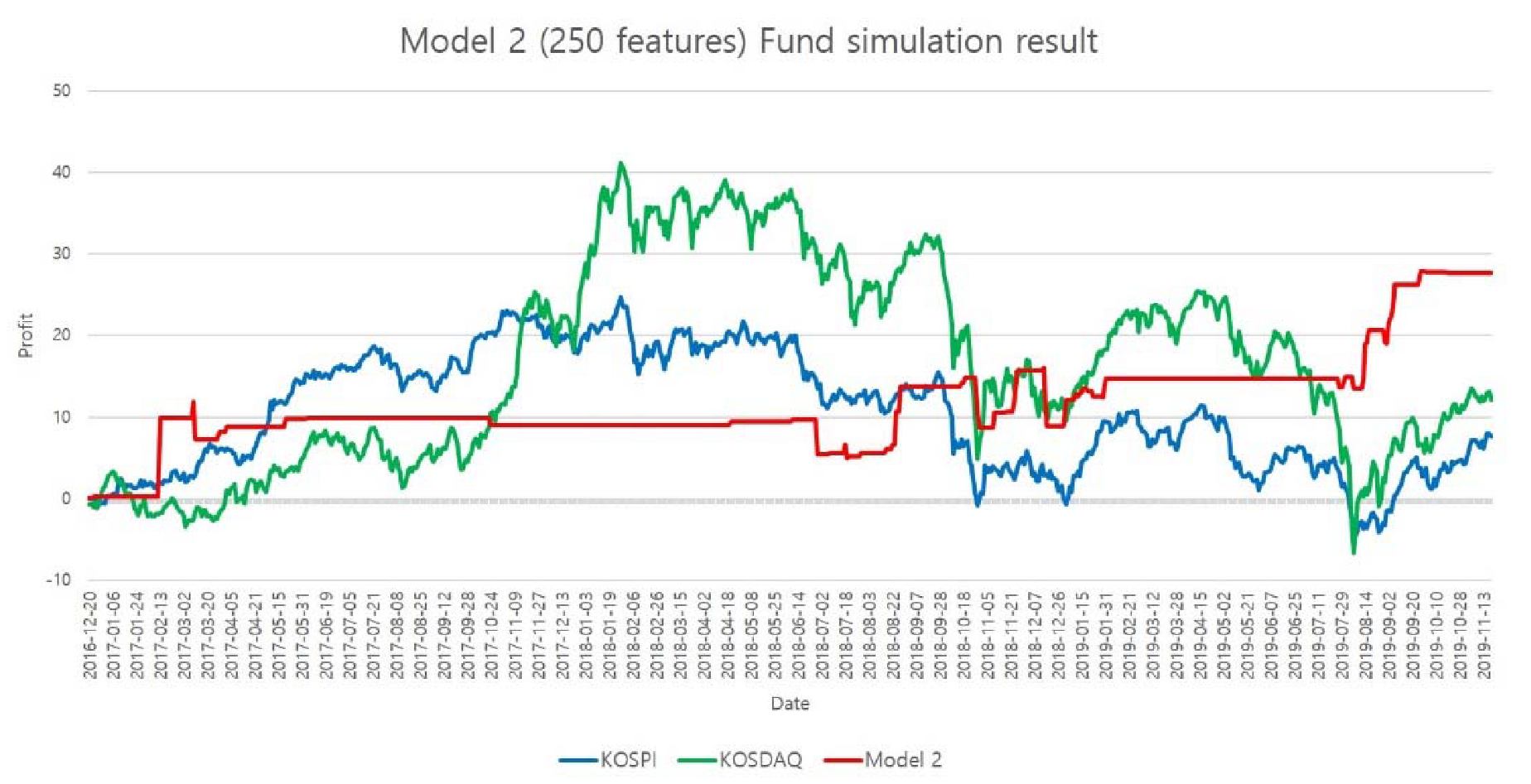
The stock symbol and recommended date according to prediction results may not come out every day, but may come intermittently. Therefore, we do not trade stocks on days when recommendations are not available. A non-trading day corresponds to a flat section of the profit graph in Figure 4 and Figure 5. We conduct the fund simulation results only when the recommendations are available. For example, if the recommended stock purchased reaches +10% from the purchase price, it will be sold. If the decreasing rate falls by more than −10%, it will be also sold automatically.

Figure 4. Profit graph of Model 1.

Figure 5. Profit graph of Model 2.

Among our models, Model 2 had the best predictive performance and highest profit. This is a model that uses a combination of binary features and price features. Moreover, Model 2 had a higher return than the KOSPI/KOSDAQ and showed a profit greater than 27% for approximately 4 years. A graph of the profit of Model 2 is shown in Figure 5. Model 2 sometimes showed flat graphs when the periods have no or few recommended stocks. Nevertheless, there is clearly a relatively stable profit, and the graph continues to rise overall.

Model 3 had the highest MSE and MAE values, and the fund simulation could not be performed because the recommended stocks were not available. We think the reasons for the poor performance of Model 3 are as follows: Model 3 uses well-known indicators that many people already use for investment. In stock trading, it is difficult to obtain substantial returns on investments using well-known technical indicators that everybody knows.

6. Conclusions

Most of the stock price prediction studies use simple price values, such as closing price, high price, low price, and volume. Conversely, in the image recognition field, implicit feature values are extracted through convolution and pooling to perform deep learning. High-performance image recognition models can be created through this process.

Therefore, we believe that we can develop a stock price prediction model with better performance by constructing meaningful features instead of using simple price features. Based on this, we proposed three models. Model 1 was developed through input feature refinement and normalization. The second model utilizes event binary features. The crucial investment points found in the charts are represented by event binary features, which are used as input for Model 2. Finally, the third model uses well-known technical analysis indicators. We valuated these three models under the same experimental conditions. As a result of the performance verification, all three models showed low error. The MSE value ranged from 0.0795 to 0.1171. The MAE value ranged from 0.2162 to 0.2498. Model 2 had the lowest error. Moreover, we performed additional fund simulations because it requires more than low error to be a good model. As a result, we could obtain some profit from Model 1 and Model 2. Among them, Model 2 was able to earn more profit than the domestic stock index, KOSPI/KOSDAQ.

In conclusion, a model with binary features is most effective, and binary features that have event moments can play a critical role in deep learning stock price prediction. Some researchers argue that stock price prediction must reflect social economic situations, but our experiment results have proved that sufficient profit can be generated using only numerical data that consist of binary event features and well-tuned features based on technical analysis. If we use Model 1 or Model 2 developed in this study, we can obtain recommendations of stocks that are expected to rise.

Finally, we believe our conclusions clash with the efficient market hypothesis. According to this hypothesis, the stock fluctuations are close to random because of the efficient sharing of disclosed information. This hypothesis has been confirmed by Model 3. In contrast, the input features of Model 1 and 2 are not well known, but we have derived a model that yields a better return than the market. This result means that the presentation of new input features and the event binary features can be very important factors in stock price prediction.

This study can be extended to various time series data (oil price, gold price, real estate price, etc.) in the future. In addition, it is possible to identify various factors and precautions to be considered with stock price prediction using deep learning. We plan to propose a unified platform by combining this model with an automated trading system in future studies. We would also like to apply CNN, recurrent neural network, etc., instead of a simple neural network structure. If we combine our high-performance features with more complex neural network structures, we may be able to derive better prediction models.

References

1. Phoon, K.; Koh, F. Robo-advisors and wealth management. J. Altern. Investig. 2017, 20, 79–94. [Google Scholar] [CrossRef]
2. Kaya, O.; Schildbach, J.; Schneider, S. Robo-Advice–A True Innovation in Asset Management. Deutsche Bank Research. Available online: https://www.dbresearch.com/PROD/DBR_INTERNET_EN-PROD/PROD0000000000449010/Robo-advice_-_a_true_innovation_in_asset_managemen.pdf (accessed on 21 February 2020).
3. Lim, H.; Ryu, D.; Yang, H. Economic analysis of robo-advisor industries: A case study. Korean Acad. Soc. Bus. Admin. 2018, 47, 725–749. [Google Scholar]
4. Trading Economics. Available online: https://tradingeconomics.com/united-states/interest-rate (accessed on 13 June 2019).
5. Blenman, L.P. Market liberalization and trading in Korea. Int. J. Bank. Financ. 2020, 7, 37–58. [Google Scholar]
6. Bollerslev, T.; Wright, J.H. High-frequency data, frequency domain inference, and volatility forecasting. Rev. Econ. Stat. 2001, 83, 596–602. [Google Scholar] [CrossRef]
7. Song, Y.; Lee, J.W.; Lee, J.W. A study on novel filtering and relationship between input-features and target-vectors in a deep learning model for stock price prediction. Appl. Intell. 2019, 49, 897–911. [Google Scholar] [CrossRef]
8. Arora, N. Financial Analysis: Stock Market Prediction Using Deep Learning Algorithms. In Proceedings of the International Conference on Sustainable Computing in Science, Technology and Management (SUSCOM), Jaipur, India, 26–28 February 2019. [Google Scholar]
9. Sim, H.S.; Kim, H.I.; Ahn, J.J. Is deep learning for image recognition applicable to stock market prediction? Complexity 2019, 2019, 1–10. [Google Scholar] [CrossRef]
10. Bollen, J.; Mao, H.; Zeng, X. Twitter mood predicts the stock market. J. Comput. Sci. 2011, 2, 1–8. [Google Scholar] [CrossRef]
11. Schumaker, R.P.; Chen, H. Textual analysis of stock market prediction using breaking financial news: The azfin text system. ACM Trans. Inf. Syst. 2009, 27. [Google Scholar] [CrossRef]
12. Naeini, M.P.; Taremian, H.; Hashemi, H.B. Stock Market Value Prediction Using Neural Networks. In Proceedings of the 2010 International Conference on Computer Information Systems and Industrial Management Applications (CISIM), Krackow, Poland, 8–10 October 2010; pp. 132–136. [Google Scholar]
13. JuHyok, U.; Lu, P.; Kim, C.; Ryu, U.; Pak, K. A new LSTM based reversal point prediction method using upward/downward reversal point feature sets. Chaos Solitons Fractals 2020, 132, 109559. [Google Scholar]
14. Rajput, V.; Bobde, S. Stock market forecasting techniques: Literature survey. Int. J. Comput. Sci. Mob. Comput. 2016, 5, 500–506. [Google Scholar]
15. Song, Y.; Lee, J.W. Implementation of Chart Type Filtering for Stock Price Prediction. In Proceedings of the KCC 2018, Seoul, Korea, 20–22 June 2018; pp. 680–682. [Google Scholar]
16. Rosenblatt, F.X. Principles of Neurodynamics: Perceptrons and the Theory of Brain Mechanisms; Spartan Books: Washington, DC, USA, 1961. [Google Scholar]
17. Rumelhart, D.E.; Hinton, G.E.; Williams, R.J. Learning representations by back-propagating errors. Nature 1986, 323, 533–536. [Google Scholar] [CrossRef]
18. Ahmar, A. Sutte Indicator: A Technical Indicator in Stock Market. Int. J. Econ. Financ. Issues 2017, 7, 223–226. [Google Scholar]
19. Tkacz, G. Neural network forecasting of Canadian GDP growth. Int. J. Forecast. 2001, 17, 57–69. [Google Scholar] [CrossRef]
20. Lee, J.W.; Kim, S.Y.; Kim, S.D.; Lee, J.W.; Chae, J.S. A two-phase stock trading system based on pattern matching and automatic rule induction. Korean Inf. Process. Soc. 2003, 10, 257–264. [Google Scholar]
21. Wong, W.K.; Manzur, M.; Chew, B.K. How rewarding is technical analysis? Evidence from Singapore stock market. Appl. Financ. Econ. 2003, 13, 543–551. [Google Scholar] [CrossRef]
22. Rosillo, R.; De la Fuente, D.; Brugos, J.A.L. Technical analysis and the Spanish stock exchange: Testing the RSI, MACD, momentum and stochastic rules using Spanish market companies. Appl. Econ. 2013, 45, 1541–1550. [Google Scholar] [CrossRef]
23. Lawrance, A.J.; Lewis, P.A.W. An exponential moving-average sequence and point process (EMA1). J. Appl. Probab. 1977, 14, 98–113. [Google Scholar] [CrossRef]
24. Yu, L.; Wang, S.; Lai, K.K. Mining stock market tendency using GA-based support vector machines. In International Workshop on Internet and Network Economics; Springer: Berlin/Heidelberg, Germany, 2015; pp. 336–345. [Google Scholar]
25. Bollinger Band Definition. Available online: https://www.investopedia.com/terms/b/bollingerbands.asp (accessed on 20 February 2020).
26. Bollinger, J. Using Bollinger bands. Stock. Commod. 1992, 10, 47–51. [Google Scholar]
27. Ferri, C.; Hernández-Orallo, J.; Salido, M.A. Volume under the ROC surface for multi-class problems. In European Conference on Machine Learning; Springer: Berlin/Heidelberg, Germany, 2003; pp. 108–120. [Google Scholar]
28. Auer, P.; Jaksch, T.; Ortner, R. Near-optimal regret bounds for reinforcement learning. J. Mach. Learn. Res. 2010, 11, 1563–1600. [Google Scholar]
29. Watkins, C.J.; Dayan, P. Q-learning. Mach. Learn. 1992, 8, 279–292. [Google Scholar] [CrossRef]
30. Iglewicz, B. Robust Scale Estimators and Confidence Intervals for Location; Wiley: New York, NY, USA, 1983; p. 417. [Google Scholar]
31. Jin, J.; Li, M.; Jin, L. Data normalization to accelerate training for linear neural net to predict tropical cyclone tracks. Math. Probl. Eng. 2015, 931629. [Google Scholar] [CrossRef]
32. Aryal, D.R.; Wang, Y.W. Neural network forecasting of the production level of Chinese construction industry. J. Comp. Int. Manag. 2003, 6, 45–64. [Google Scholar]
33. Dilli, R.; Wang, Y.W. An application of the ARIMA model for forecasting the production level of construction industry. J. Harbin Inst. Technol. 2002, 9, 39–45. [Google Scholar]
34. Lee, J.W. Integrated multiple simulation for optimizing performance of stock trading systems based on neural networks. KIPS Trans. B 2007, 14, 127–134. [Google Scholar] [CrossRef]
Article Metrics
Citations
Article Access Statistics
Multiple requests from the same IP address are counted as one view.