Abstract
Colorectal cancer is ranked third and fourth in terms of mortality and cancer incidence in the world. While advances in treatment strategies have provided cancer patients with longer survival, potentially harmful second primary cancers can occur. Therefore, second primary colorectal cancer analysis is an important issue with regard to clinical management. In this study, a novel predictive scheme was developed for predicting the risk factors associated with second colorectal cancer in patients with colorectal cancer by integrating five machine learning classification techniques, including support vector machine, random forest, multivariate adaptive regression splines, extreme learning machine, and extreme gradient boosting. A total of 4287 patients in the datasets provided by three hospital tumor registries were used. Our empirical results revealed that this proposed predictive scheme provided promising classification results and the identification of important risk factors for predicting second colorectal cancer based on accuracy, sensitivity, specificity, and area under the curve metrics. Collectively, our clinical findings suggested that the most important risk factors were the combined stage, age at diagnosis, BMI, surgical margins of the primary site, tumor size, sex, regional lymph nodes positive, grade/differentiation, primary site, and drinking behavior. Accordingly, these risk factors should be monitored for the early detection of second primary tumors in order to improve treatment and intervention strategies.
1. Introduction
Worldwide, colorectal cancer is considered one of the top three causes of cancer-related deaths in developed countries [1]. Due to the success of cancer screening, the early detection and diagnosis of malignant tumors have become feasible. In addition, due to advances in therapeutic instruments and techniques, such as three-dimensional spatial conformal radiation therapy, intensity-modulated radiation therapy, and proximity radiation therapy, cancer patients have longer survival. However, there is a risk of the occurrence of potentially harmful second primary cancers (SPCs) [2,3,4].
Five-year cancer survival rates have historically been an important indicator of clinical treatment. One of the most difficult clinical issues for cancer survivors is the occurrence of multiple primary malignant neoplasms (MPMNs). Multiple malignancies are characterized by two or more independent primary malignancies diagnosed in different tissues/organs in the same individual [5]. In general, MPMNs are most present in double cancers. According to the literature, the incidence of second primary malignant tumors in patients with malignant tumors is six times higher than that in healthy people. Second primary malignant tumors occur most often within 3 years of the first tumor treatment; the shorter the interval between the first cancer and the SPC, the worse the prognosis [6]. The prevention of MPMNs has always been a significant problem faced by both doctors and patients. The high prevalence age range for MPMNs is 50–59, with most patients being over 50 years old [2].
The first research report on MPMNs was published by Warren and Gates in 1932. According to their definition, MPMNs should have first and second malignant tumors; there should be at least 2 cm between the two tumors; they should exclude metastatic tumors occurring within 5 years; and occurring at a time more than 3 years after the primary tumor [7]. The definition of SPC (synchronous vs, metachronous) is based on the diagnosed time of the first primary cancer. Accordingly, primary cancers found within 6 months of the first diagnosis are considered to be synchronous, whereas metachronous cancers refer to primary cancers discovered 6 months after the first diagnosis [8]. In general, cancer treatment is characterized followed by the targeted therapy and palliative treatment. The treatment target can be divided into cancer-free survival and chronic comorbid management. The latter can result in treatment failure, leading to palliative treatment, and in more severe cases, to an SPC [9].
According to the guidelines of the Institute of Medicine’s prevention and treatment recommendations for multiple malignancies, “Based on the cancer-registered population, it is imperative to use the empirical medical perspective and systematic analysis of therapeutic techniques to further develop clinical treatment guidelines for multiple malignancies (MPMNs)” [10].
With recent developments in information technology, data classification methods represent an important research field and have also become useful tools to support clinical diagnostic guidelines. Machine learning is one of the most used data mining methods, and has been applied to analyze important information hidden in the vast amount of data stored in medical databases. There are many different kinds of machine learning methods used for building predictive models for cancer classification/prediction. For example, Tseng et al. [11] used a support vector machine (SVM) and extreme learning machine (ELM) to predict the recurrence-proneness of cervical cancer. Tseng et al. [12] utilized SVM, ELM, multivariate adaptive regression splines (MARS), and random forest (RF) to identify risk factors and diagnose ovarian cancer recurrence. Ting et al. [13] also applied SVM, ELM, MARS, and the RF method to detect recurrence in patients diagnosed with colorectal cancer. Chang and Chen [14] proposed a classification model using extreme gradient boosting (XGBoost) as the classifier for predicting second primary cancers in women with breast cancer. MARS, SVM, ELM, RF, and XGBoost methods have achieved good performances for constructing effective predictive models of cancer. In addition, gene expression classifiers are currently being used in therapeutic intervention. Kopetz et al. [15] developed ColoPrint prediction method for improving prognostic accuracy independent of microsatellite status. Gao et al. [16] developed cancer hallmark-based gene signature sets (CSS sets) for prognostic predictions and for facilitating the identification of patients with stage II colorectal cancer. Since they are based on different concepts, involving nonparametric statistics, statistical learning, a neural network, and a decision tree, to make effective algorithms with different characteristics for cancer data analysis, they are used in this study for analyzing SPCs in colorectal cancer.
Over the last two decades, cancer registration databases have been used to store records related to the treatment of colorectal cancer patients. Indeed, a vast network of useful information is hidden in these collected datasets. Although traditional data query and statistical functions can be utilized, such as prediction of primary colorectal cancer by National Cancer Institute’s Surveillance, Epidemiology, and End Results (SEER) data [17]. Statistic methods such as the chi-square test and Student’s t-test were used in univariate statistical analysis, and the Kaplan-Meier method and log-rank test are used for continued variables in traditional medical articles [18,19]. It is not easy to find unknown information features in practice, and information about their potential value cannot be directly observed from the dataset. As such, how to explore hidden, unknown, and valuable information from SPC databases through specific procedures and methods is an important research topic that aims to improve prevention and treatment strategies for colorectal cancer survivors.
In this study, we used five machine learning techniques to develop a predictive model for the SPC among colorectal cancer patients. The model can be used to identify various analyzable risk factors and clinical features within primary tumors, providing decision support for intensive treatments such as adjuvant chemotherapy, or aggressive following up procedures, such as positron emission tomography (PET).
2. Methods
2.1. MARS
Multivariate adaptive regression splines (MARS) is a flexible procedure used to find optimal variable transformations and interactions. It can be used to identify model relationships that are nearly additive or that involve interactions with fewer variables. MARS is a nonparametric statistical method based on a divide-and-conquer strategy for partitioning training datasets into separate groups, each of which gets its own regression equation. The non-linearity of the MARS model is approximated via the use of separate linear regression slopes in distinct intervals of the independent variable space.
The MARS function is a weighted sum of the basis functions (BFs), which are splines piecewise polynomial functions. It can be represented using the following equation [20]:
where and are constant coefficients that can be estimated using the least-squares method. M is the number of basis functions. represents the basis functions. The hinge functions, or , with a knot defined at value t, are used in MARS modeling. In addition, MARS automatically selects the variables and values of those variables for knots of the hinge functions based on generalized cross-validation criterion [21].
2.2. RF
Random forest (RF) is an ensemble classification method that combines several individual classification trees [22,23]. RF is a supervised machine learning algorithm that considers the unweighted majority of the class votes. First, various random samples of variables are selected as the training dataset using the bagging procedure, which is a meta-algorithm that uses random sampling with replacement to synchronously reduce variance and elude over-fitting. Classification trees using selected samples are then built into the training process. A large number of classification trees are then used to form a RF from the selected samples. Classification and regression tree (CART) is typically the classification method used for RF modeling. Finally, all classification trees are combined and the final classification results are obtained by voting on each class and then choosing the winner class in terms of the number of votes. RF performance is measured by a metric called “out of bag” error, which is calculated as the average of the rate of error for each weak learner. In RF, each individual tree is explored in a particular way. The most important variable randomly chosen is used as a node and each tree is developed to its maximum expansion [22].
2.3. SVM
Support vector machine (SVM) is a machine learning algorithm based on the structural risk minimization principle for estimating a function by minimizing the upper bound of the generalization error [24]. In modeling an SVM model, one can initially use the kernel function to, either linearly or non-linearly, map the input vectors into one feature space. Then, within the feature space, the SVM attempts to seek an optimized linear division to construct a hyperplane that separates the classes. In order to optimize the hyperplane, SVM solves the optimization problem using the following equation [24]:
where is the input variable, is the known target variable, is the number of sample observations, is the dimension of each observation, is the vector of the hyperplane, and is a bias term.
In order to solve Equation (2), the Lagrange method is used to transform the optimization problem into a dual problem. The penalty factor is used as a tuning parameter in the transformed dual problem to control the trade-off between maximizing the margin and the classification error. In general, SVM does not find the linear separate hyperplane for all application data. For non-linear data, it must transform the original data to a higher dimension of linearity separately as the best solution. The higher dimension is called the feature space and it improves the data separated by classification. The common kernel functions are linear, polynomial, radial basis function, and sigmoid. Although several choices for the kernel function are available, the most widely used is the radial basis function kernel [25].
2.4. ELM
Extreme learning machine (ELM) is a single hidden layer feed-forward neural-network (SLFN) that randomly selects the input weights and analytically determines the output weights of the SLFN [26]. The modeling time of ELM is faster than traditional feedforward network learning algorithms such as the back-propagation (BP) algorithm. It also avoids many difficulties present in gradient-based methods, such as the stopping criteria, learning rate, learning epochs, local minimal, and over tuning issues.
In SLFNs, represents the arbitrary distinct samples (), using hidden neurons and the activation function vector and approximates samples with zero error, written as:
where is the hidden layer output matrix of the neural network and the i-th column of ; is the matrix of the output weights; is the weight vector connecting the i-th hidden node and the input nodes; is the threshold (bias) of the i-th hidden node; and is the matrix of the targets.
Huang et al. [26] demonstrated that the input weights and hidden layer biases can be randomly generated in the ELM algorithm, and the output weights can be determined as simply as finding the least-square solution to a given linear system. Accordingly, the minimum norm least-square solution to the linear system is , where is the Moore-Penrose generalized inverse of the matrix . The minimum norm least-square solution is unique and has the smallest norm among all least-square solutions [26].
2.5. XGboost
XGBoost belongs to the group of widely used tree learning algorithms. It is a supervised learning algorithm based on a scalable end-to-end gradient tree boosting system [27]. Boosting refers to the ensemble learning technique of building many models sequentially, with each new model attempting to correct for the imperfections or inadequacies in the previous model. In other words, in gradient boosting, a new weak learner is constructed to be maximally correlated with the negative gradient of the loss function associated with the whole assembly for each iteration [28].
XGBoost is the implementation of a generalized gradient boosting decision tree that uses a new distributed algorithm for tree searching, which speeds up tree construction. XGBoost includes a regularization term that is used to alleviate overfitting, and as support for arbitrary differentiable loss functions [29]. The objective function of Xgboost consists of two parts; namely, a loss function over the training set and a regularization term that penalizes the complexity of the model as follows [30]:
where can be any convex differentiable loss function that measures the difference between the prediction and the true label for a given training instance. describes the complexity of the tree and is defined in the XGBoost algorithm as:
where is the number of leaves on tree and is the weight of the leaves. When is included in the objective function, it is forced to optimize for a less complex tree, which simultaneously minimizes . This helps to alleviate any overfitting issues. provides a constant penalty for each additional tree leaf, and penalizes for extreme weights. and are user configurable parameters [30].
2.6. Model Implementation
The five machine learning methods have been implemented in the R of version 3.6.1 (R core team, Vienna, Austria). The algorithm used for each method is based on that applied in the corresponding R package. In the first method, MARS was implemented using earth R package of version 5.1.2 [31]. The default setting of this package was used; all variables were included to build an additive MARS model. Second, the randomForest R package of version 4.6.14 was used for constructing RF classification models [32]. Using the default setting, each forest was built with 500 trees. The best value of the minimum number of variables randomly sampled as candidates at each split is searched from the square root of total number of predictors to the number of predictors. Third, SVM classification models were built by using e1071 R package of version 1.7-1 [33]. The radial basis kernel function with the gamma parameter at its default setting was used this study. In order to find the best parameter set of cost and gamma parameters for building effective SVM models, the tune function of e1071 R package was applied. Fourth, for building ELM models, the elmNN R package of version 1.0 was used [34]. The default used activation function in this package is radial basis. To search the best number of hidden neurons which can generate promising ELM models, caret R package of version 6.0-84 was implemented [35]. For the fifth method, XGBoost model was constructed by implementing xgboost R package of version 0.90.0.2 [36]. To estimate the best parameter set for building effective XGBoost models, caret R package of version 6.0-84 was also used for tuning the six important hyper-parameters: the maximum number of boosting iterations, learning rate, minimum loss reduction, maximum depth of a tree, subsample ratio of the training instances, and subsample ratio of features.
3. Proposed Prediction Scheme
In this study, the five machine learning classification techniques described above were integrated to propose a scheme for predicting SPC in colorectal cancer patients. The flowchart of the proposed scheme is shown in Figure 1.
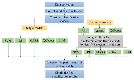
Figure 1.
The flowchart of the proposed second primary cancer (SPC) prediction scheme in colorectal cancer patients.
The first step of the proposed scheme was to collect the data. The second step was to collect candidate risk factors as predictor variables. In addition, this paper reviews the available literature on what variables are associated with the risk factors for the recurrence of ovarian cancer [13]. As shown in Table 1, the 14 risk factors for SPC in colorectal cancer patients are represented as X1 to X14. The target variable is SPC or not (Y).

Table 1.
The fourteen candidate risk factors for SPC in colorectal cancer patients.
In the third step, we constructed classification models for predicting SPC in colorectal cancer patients. In building the classification models, we used two types of modeling processes. One was a single model and the other was a two-stage model. In modeling the single models, all 14 risk factors were directly used as predictors for SVM, RF, MARS, ELM, and XGboost for constructing five single classification models. These were termed single SVM (S-SVM), single RF (S-RF), single MARS (S-MARS), single ELM (S-ELM), and single XGboost (S-XGboost) models.
The two-stage model integrating the feature selection method and classifier were used in the third step of the proposed scheme, as important disease risk factors are often fundamental indicators that provide useful information for modeling effective disease predictions. In modeling the two-stage model, a feature selection method was first used to select the important risk factors. Among the five machine learning methods, only RF, MARS, and XGboost can be used to select important risk factors based on their fundamental algorithms; thus, these were used as the three feature selection methods to identify and rank important risk factors for predicting SPC in colorectal cancer patients. Each feature selection method generated one set of important risk factors. Using only one feature selection technique may not provide stable and effective selection results. A simple average rank method was used to combine the risk factor selection results of the three methods.
Table 2 shows the selected and ranked risk factors using the RF, MARS, and XGboost methods. Note that a risk factor with a rank of 1 indicates that it is the most important risk factor, while one with a rank of 14 indicates that it is a risk factor not selected by the method. For each risk factor, the average rank was obtained by calculating the average value of its rankings in the RF, MARS, and XGboost methods. Table 2 shows, also, the average rank of every risk factor. The ranked overall variable importance of all the risk factors is shown in Figure 2. It can be observed that X7, with an average rank of 1, is the most important risk factor, followed by X2 and X11.
Table 2.
The selected and ranked risk factors using the RF, MARS, and XGboost methods.
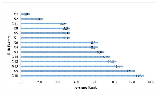
Figure 2.
The ranking of all risk factors.
In the modeling process of the two-stage method, after obtaining the average rank of each risk factor, the overall important risk factors should be identified before constructing a classification model. In this study, an average rank value less than 10 was used as the criterion for selecting the overall important risk factors. This criterion was determined by the suggestion of clinical physicians. Based on this criterion, it can be observed from Figure 2 that the 10 risk factors including X7 (combined stage), X2 (age at diagnosis), X11 (BMI), X8 (surgical margins of the primary site), X5 (tumor size), X1 (sex), X6 (regional lymph nodes positive), X4 (grade/differentiation), X3 (primary site), and X14 (drinking), were selected as the important risk factors.
In the final stage of the two-stage method, the identified 10 overall important risk factors served as the input variables for the SVM, RF, MARS, ELM, and XGboost methods in order to predict SPC in colorectal cancer patients. The five two-stage methods were termed A-SVM, A-RF, A-MARS, A-ELM, and A-XGboost, respectively.
In the fourth step of the proposed scheme, after obtaining the classification results from the five single methods and the five two-stage methods, we used accuracy, sensitivity, specificity, and area under the curve (AUC) parameters as classification accuracy metrics to compare the performances of the ten models.
In the final step, after comparing the classification performances of the ten models, including S-SVM, S-RF, S-MARS, S-ELM, S-XGboost, A-SVM, A-RF, A-MARS, A-ELM, and A-XGboost models, we obtained the final diagnosis results and identified the important risk factors for predicting SPC in colorectal cancer patients.
This study used 10-fold cross validation methods to estimate the performances of the proposed ten models. First, we randomly split the whole dataset into 10 equal sized parts, with nine folds as the training data set and one fold as the testing data set. That was repeated 10 times, with each of the 10 folds used exactly once as the testing data set. The ten results of classification accuracy metrics could then be averaged to produce the final performances of the methods.
4. Empirical Results
In this study, colorectal cancer datasets provided by three hospital cancer registries were used to verify the proposed medical diagnostic scheme for predicting the occurrence of SPC in colorectal cancer patients. Each patient in the dataset had 14 predictor variables, with one response variable indicating SPC or not. Excluding incomplete records, there were a total of 4287 patients in the dataset. The 10-fold cross-validation method was used in this study for evaluating the performance of the proposed scheme. This received institutional review board (IRB) approval by the Chung-Shan Medical University Hospital (CSMUH number: CS18116).
For modeling the ten models, including the S-SVM, S-RF, S-MARS, S-ELM, S-XGboost, A-SVM, A-RF, A-MARS, A-ELM, and A-XGboost models for predicting SPC in colorectal cancer patients, the process mentioned in Section 3 was used. Table 3 shows the classification results of the five single methods, including the S-SVM, S-RF, S-MARS, S-ELM, and S-XGboost models. From Table 3, it can be observed that the AUC values of the S-SVM, S-RF, S-MARS, S-ELM, and S-XGboost models were 0.711, 0.618, 0.640, 0.710, and 0.550, respectively. The single SVM model provided the highest AUC value, followed by the single XGboost model with a slightly smaller AUC value. However, it also can be seen from Table 3 that the accuracy value of the S-XGboost model was 0.641, which is significantly greater than that of the single SVM model at 0.408. Figure 3 shows the ROC (Receiver Operating Characteristic) curves of the five single classification methods for the occurrence of SPC in colorectal cancer patients. Thus, among the five single classification methods, the single XGboost model provided the best classification results.
Table 3.
Classification results of the five single methods.
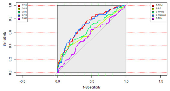
Figure 3.
ROC (Receiver Operating Characteristic) curves of the five single methods.
As aforementioned, the 10 risk factors, including X7, X2, X11, X8, X5, X1, X6, X4, X3, and X14, were selected as the important risk factors and then served as the critical predictor variables for constructing the five two-stage methods, including the A-SVM, A-RF, A-MARS, A-ELM, and A-XGboost models.
Table 4 shows the classification accuracy matrices of the five two-stage methods. As depicted in Table 4, it can be observed that the A-XGboost method generated the highest AUC value at 0.714, with a sensitivity value of 0.767, compared with the competing models. Figure 4 displays the ROC curves of the five two-stage methods. From Table 4 and Figure 4, it can be observed that the A-XGboost method generated the best performance for predicting the occurrence of SPC in colorectal cancer patients and is the best method among the five two-stage models.
Table 4.
Classification results of the five two-stage methods.
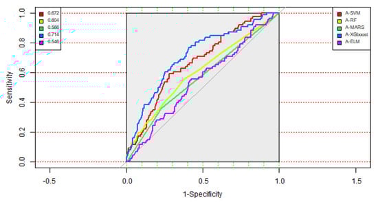
Figure 4.
ROC curves of the five two-stage methods.
For comparing the classification performances between the five single methods and the five two-stage models, Figure 5 depicts the AUC values of the ten models in decreasing order. It can be observed from Figure 5 that the A-XGboost model generated the best AUC value, followed by the S-SVM and S-XGboost models. These results indicated that the A-XGboost method is a good alternative for constructing a classification model for diagnosing the occurrence of SPC in colorectal cancer. Moreover, the A-XGboost method can be used to select important risk factors that are more influential on patients with SPC of colorectal cancer.
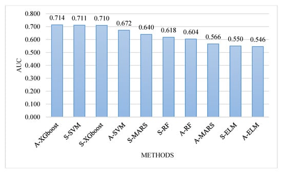
Figure 5.
Comparison of the area under the curve (AUC) values of the ten models.
In order to evaluate the robustness of the ten models, we randomly repeated 10-fold cross-validation 100 times and averaged the classification accuracy metrics; i.e., accuracy, sensitivity, specificity, and AUC. The averaged accuracy, sensitivity, specificity, and AUC values are shown in Table 5. From the Table, it can be observed that the A-XGboost model still generated the highest AUC value, 0.723, and is the most promising model in this study for predicting the SPC in colorectal cancer.
Table 5.
Evaluation of the ten models based on the averaged classification results.
5. Discussion and Conclusions
In this study, 10 important risk factors, including the combined stage, age at diagnosis, BMI, surgical margins of the primary site, tumor size, sex, regional lymph nodes positive, grade/differentiation, primary site, and drinking behavior, were selected by the A-XGboost model, which provided the best classification performance among the ten models constructed in this study.
Colorectal cancer ranks second and third in terms of mortality and incidence, respectively, in Taiwan. It is also the third highest cancer in terms of medical expenditure. While patient survival has improved, the occurrence of second primary cancers in colorectal cancer patients has become an important issue for clinical management. A variety of different ML techniques have been used in the medical study over the last two decades. To address this issue, data from the cancer registry can be used to better understand the disease and maximize the prevention of SPC. Important issues for future research include predictive models (radiotherapy and chemotherapy) and their association with SPC, as well as a better understanding of the interactions with other genetic factors. Besides, the hospital based cancer registry can be easily extended to the national cancer registry easily. Further discussion with patients after diagnosis should help determine the optimal duration of monitoring and follow-up in early detecting the second primary cancer.
Author Contributions
W.-C.T. compiled the data set and drafted the manuscript; H.-R.C. participated in the experimental design and drafted the manuscript; C.-C.C. edited the manuscript and conceived the study; C.-J.L. wrote the experimental programs and conceived the study. All authors have read and agreed to the published version of the manuscript.
Funding
This work is supported by the Chung-Shan Medical University Hospital: CSH-2020-C-020 and Ministry of Science and Technology, Taiwan, R.O.C. under grant numbers 107-2221-E-040 -009 – and 107-2221-E-231-002.
Conflicts of Interest
The authors declare no conflicts of interest.
References
- Zinatizadeh, N.; Khalili, F.; Fallah, P.; Farid, M.; Geravand, M.; Yaslianifard, S. Potential preventive effect of lactobacillus acidophilus and lactobacillus plantarum in patients with polyps or colorectal cancer. Arq. Gastroenterol. 2018, 55, 407–411. [Google Scholar] [CrossRef] [PubMed]
- Sakellakis, M. Multiple primary malignancies: A report of two cases. Chin. J. Cancer Res. 2014, 26, 215–218. [Google Scholar] [PubMed]
- Santangelo, M.L. Immunosuppression and multiple primary malignancies in kidney-transplanted patients: A single-institute study. BioMed Res. Int. 2015, 2015, 183–523. [Google Scholar] [CrossRef]
- Xu, W. Multiple primary malignancies in patients with hepatocellular carcinoma: A largest series with 26-year follow-up. Medicine 2016, 95, e3491. [Google Scholar] [CrossRef] [PubMed]
- Li, F. Multiple primary malignancies involving lung cancer. BMC Cancer 2015, 15, 696. [Google Scholar] [CrossRef] [PubMed]
- Wu, L.L.; Gu, K.S. Clinical retrospective analysis of cases with multiple primary malignant neoplasms. Genet. Mol. Res. 2014, 13, 9271–9284. [Google Scholar]
- Meng, L.V.; Zhang, X.; Shen, Y.; Wang, F.; Yang, J.; Wang, B.; Chen, Z.; Li, P.; Zhang, X.; Li, S.; et al. Clinical analysis and prognosis of synchronous and metachronous multiple primary malignant tumors. Medicine 2017, 96, e6799. [Google Scholar]
- Huang, C.S.; Yang, S.H.; Lin, C.C.; Lan, Y.T.; Chang, S.C.; Wang, H.S.; Chen, W.S.; Lin, T.C.; Lin, J.K.; Jiang, J.K. Synchronous and metachronous colorectal cancers: Distinct disease entities or different disease courses? Hepato Gastroenterol. 2015, 62, 838–842. [Google Scholar]
- Patricia, A.G.; Jacqueline, C.; Erin, E.H. Ensuring quality care for cancer survivors: Implementing the survivorship care plan. Semin. Oncol. Nurs. 2015, 24, 208–217. [Google Scholar]
- Vogt, A.; Schmid, S.; Heinimann, K.; Frick, H.; Herrmann, C.; Cerny, T.; Omlin, A. Multiple primary tumours: Challenges and approaches, a review. ESMO Open 2017, 2, e000172. [Google Scholar] [CrossRef]
- Tseng, C.J.; Chang, C.C.; Lu, C.J.; Chen, G.D. Application of machine learning to predict the recurrence-proneness for cervical cancer. Neural Comput. Appl. 2014, 24, 1311–1316. [Google Scholar] [CrossRef]
- Tseng, C.J.; Lu, C.J.; Chang, C.C.; Chen, G.D.; Cheewakriangkrai, C. Integration of data mining classification techniques and ensemble learning to identify risk factors and diagnose ovarian cancer recurrence. Artif. Intell. Med. 2017, 78, 47–54. [Google Scholar] [CrossRef] [PubMed]
- Ting, W.C.; Lu, Y.C.; Lu, C.J.; Cheewakriangkrai, C.; Chang, C.C. Recurrence impact of primary site and pathologic stage in patients diagnosed with colorectal cancer. J. Qual. 2018, 25, 166–184. [Google Scholar]
- Chang, C.C.; Chen, S.H. Developing a novel machine learning-based classification scheme for predicting SPCs in breast cancer survivors. Front. Genet. 2019, 10, 848. [Google Scholar] [CrossRef] [PubMed]
- Kopetz, S.; Tabernero, J.; Rosenberg, R.; Jiang, Z.Q.; Moreno, V.; Bachleitner-Hofmann, T.; Lanza, G.; Stork-Sloots, L.; Maru, D.; Simon, I.; et al. Genomic classifier ColoPrint predicts recurrence in stage II colorectal cancer patients more accurately than clinical factors. Oncologist 2015, 20, 127–133. [Google Scholar] [CrossRef] [PubMed]
- Gao, S.; Tibiche, C.; Zou, J.; Zaman, N.; Trifiro, M.; O’Connormccourt, M.; Wang, E. Identification and construction of combinatory cancer hallmark-based gene signature sets to predict recurrence and chemotherapy benefit in stage II colorectal cancer. JAMA Oncol. 2016, 2, 37–45. [Google Scholar] [CrossRef] [PubMed]
- Yang, L.; Xiong, Z.; Xie, Q.K.; He, W.; Liu, S.; Kong, P. Second primary colorectal cancer after the initial primary colorectal cancer. BMC Cancer 2018, 18, 931. [Google Scholar] [CrossRef]
- Sun, L.C.; Tai, Y.Y.; Liao, S.M.; Lin, T.Y.; Shih, Y.L.; Chang, S.F. Clinical characteristics of second primary cancer in colorectal cancer patients: The impact of colorectal cancer or other second cancer occurring first. World J. Surg. Oncol. 2014, 12, 73. [Google Scholar] [CrossRef][Green Version]
- Ringland, C.L.; Arkenau, H.T.; O’Connell, D.L.; Ward, R.L. Second primary colorectal cancers (SPCRCs): Experiences from a large Australian Cancer Registry. Ann. Oncol. 2010, 21, 92–97. [Google Scholar] [CrossRef]
- Friedman, J.H. Multivariate adaptive regression splines. Ann. Stat. 1991, 19, 1–141. [Google Scholar] [CrossRef]
- Zhang, W.; Goh, A.T. Multivariate adaptive regression splines and neural network models for prediction of pile drivability. Geosci. Front. 2016, 7, 45–52. [Google Scholar] [CrossRef]
- Breiman, L. Random forests. Mach. Learn. 2001, 45, 5–32. [Google Scholar] [CrossRef]
- Yuk, E.; Park, S.; Park, C.S.; Baek, J.G. Feature-learning-based printed circuit board inspection via speeded-up robust features and random forest. Appl. Sci. 2018, 8, 932. [Google Scholar] [CrossRef]
- Vapnik, V.N. The Nature of Statistical Learning Theory; Springer: Berlin/Heidelberg, Germany, 2000. [Google Scholar]
- Li, T.; Gao, M.; Song, R.; Yin, Q.; Chen, Y. Support vector machine classifier for accurate identification of piRNA. Appl. Sci. 2018, 8, 2204. [Google Scholar] [CrossRef]
- Huang, G.B.; Zhu, Q.Y.; Siew, C.X. Extreme learning machine: Theory and applications. Neurocomputing 2006, 70, 489–501. [Google Scholar] [CrossRef]
- Chen, T.; Guestrin, C. XGBoost: A Scalable Tree Boosting System. In Proceedings of the 22nd ACM SIGKDD International Conference on Knowledge Discovery and Data Mining, San Francisco, CA, USA, 13–17 August 2016; pp. 785–794. [Google Scholar]
- Natekin, A.; Knoll, A. Gradient boosting machines, a tutorial. Front. Neurorobotics 2013, 7, 21. [Google Scholar] [CrossRef]
- Torlay, L.; Perrone-Bertolotti, M.; Thomas, E.; Baciu, M. Machine learning–XGBoost analysis of language networks to classify patients with epilepsy. Brain Inform. 2017, 4, 159. [Google Scholar] [CrossRef]
- Mitchell, R.; Frank, E. Accelerating the XGBoost algorithm using GPU computing. PeerJ Comput. Sci. 2017, 3, e127. [Google Scholar] [CrossRef]
- Milborrow, S.; Hastie, T.; Tibshirani, R.; Miller, A.; Lumley, T. Earth: Multivariate Adaptive Regression Splines. R Package Version 5.1.2. Available online: https://www.rdocumentation.org/packages/earth (accessed on 1 October 2019).
- Liaw, A.; Wiener, M. randomForest: Breiman and Cutler’s Random Forests for Classification and Regression. R Package Version, 4.6.14. Available online: https://www.rdocumentation.org/packages/randomForest (accessed on 1 October 2019).
- Meyer, D.; Dimitriadou, E.; Hornik, K.; Weingessel, A.; Leisch, F. e1071: Misc Functions of the Department of Statistics, Probability Theory Group (Formerly: E1071), TU Wien, 2017. R Package Version, 1.7-1. Available online: https://www.rdocumentation.org/packages/e1071 (accessed on 1 October 2019).
- Gosso, A.; Martinez-de-Pison, F. elmNN: Implementation of ELM (Extreme Learning Machine) Algorithm for SLFN (Single Hidden Layer Feedforward Neural Networks). R Package Version, 1. Available online: https://www.rdocumentation.org/packages/elmNN (accessed on 1 October 2019).
- Kuhn, M.; Wing, J.; Weston, S.; Williams, A.; Keefer, C.; Engelhardt, A.; Kenkel, B. Caret: Classification and Regression Training. R Package Version 6.0-84. Available online: https://www.rdocumentation.org/packages/caret (accessed on 1 October 2019).
- Chen, T.; He, T.; Benesty, M.; Khotilovich, V.; Tang, Y. Xgboost: Extreme Gradient Boosting. R Package Version 0.90.0.2. Available online: https://www.rdocumentation.org/packages/xgboost (accessed on 1 October 2019).
© 2020 by the authors. Licensee MDPI, Basel, Switzerland. This article is an open access article distributed under the terms and conditions of the Creative Commons Attribution (CC BY) license (http://creativecommons.org/licenses/by/4.0/).