A Rapid UV/Vis Spectrophotometric Method for the Water Quality Monitoring at On-Farm Root Vegetable Pack Houses

Abstract

Our research aim was to apply UV/Vis spectrophotometric techniques for the rapid monitoring of the quality of water sourced from on-farm root vegetable washing processes. To achieve this goal, the quality assessment of the washing water and wastewater at different stages of the technological processes was performed using physicochemical, biological, and UV/Vis absorbance measurements as well as statistical methods, such as principal component analysis (PCA) and partial least squares (PLS) regression. Limit values of UV/Vis absorbance at specific wavelengths were predicted in order to adapt them for routine testing and water quality monitoring at the farm packhouses. Results of the lab analyses showed, that the main problems of the water quality were caused by suspended solids (470–3400 mg L⁻¹), organic substances (BOD₅ 215–2718 mg L⁻¹; COD 540–3229 mg L⁻¹), nitrogen (3–52 mg L⁻¹), phosphorus (1–6 mg L⁻¹), and pathogenic microorganisms (TVC > 300 cfu mL⁻¹, E. coli 5.5 × 10³–1.0 × 10⁴ cfu mL⁻¹, intestinal enterococci 2.8 × 10²–1.5 × 10⁴ cfu mL⁻¹, coliform bacteria 1.6 × 10³–2.0 × 10⁴ cfu mL⁻¹). Suspended solids exceeded the limit values by 10–50 times, organic matter by 10–25 times, dissolved organic carbon by 3–5 times, nitrogen by 3–7 times, total phosphorus by 3–12 times, and microorganisms by 3–10 times. UV/Vis limit values calculated were as follows: A210 nm—3.997–4.009 cm⁻¹, A 240 nm—5.193–5.235 cm⁻¹, A254 nm—4.042–4.047 cm⁻¹, A320 nm—7.387–7.406 cm⁻¹, and A 660 nm—3.937–3.946 cm⁻¹. UV/Vis measurements at A320 nm are proposed for the routine water quality monitoring.

1. Introduction

Washing water and wastewater quality control in on-farm packhouses is of great importance for the quality of agricultural production as well as the environment. Producers require rapid and efficient methods for water quality monitoring. Conventional standard analytical methods are expensive, time-consuming and require special laboratory conditions and equipment. Therefore they are inconvenient and impossible to use for the water quality monitoring at the on-farm packhouses. Ultraviolet/visual spectrometry (UV/Vis) can have significant advantages over other in situ methods for this application due to its wide availability and low application costs. Previously, various UV/Vis methods were used, for example, to determine the particle size of polystyrene in solution, the size distribution of quantum particles of a ZnO semiconductor, the size of gold-coated palladium clusters in solution, and to study the aggregation of b-carotene particles [1]. UV/Vis technology is rapid and can be used for the monitoring of the most important water quality parameters: total suspended solids, dissolved organic carbon, the chemical oxygen demand, the biochemical oxygen demand, and measure of detergents and nitrates, since these materials absorb electromagnetic radiation at different wavelengths (λ).

Consequently, spectrophotometry has been already proposed for the industrial wastewater quality monitoring, characterization of the organic and inorganic compounds, nitrates, detergents, dyes, as well as elements (Fe, Mn, Cr) as a fast, simple, non-destructive and inexpensive analytical method [2,3,4,5,6]. Moreover, using indirect methods of calculations can be useful in the research of wastewater microbiological activity, biomass structure, growth and biochemical processes of dissolved organic matter (DOM) reduction [7]. Recently there has been an emergence of commercially available UV/Vis spectrophotometers for the continuous optical measurements on-line and in-situ. However, the lack of selectivity and reliability of the methods remains the general restriction of these instruments for wider application [8,9,10]. UV/Vis spectrophotometry is based on Beer–Lambert law [11]:

Log I_o/I = α·c·l;

(1)

where I is the intensity of light at specific wavelength λ passing through a sample of length l, I_o is the light intensity incident on the sample, c is the concentration, and α is the absorptivity of the sample at the specific wavelength.

Between spectral and chemical data, the most common are linear and quadratic models of interactions. A linear model is as follows:

Y = ε₁c₁l + ε₂c₂l + ⋯ + ε_pc_pl + E,

(2)

where Y is the response of a particular sample at wavelength λ, ε_p is the molar extinction coefficient for the p sample, c_p is the corresponding concentration and E is the spectral error. If ε is measured at several wavelengths, then the equation obtained is:

$$Y_j({\lambda }_i)={{\displaystyle \sum }}_{\mathit{k}=\mathbf{1}}^{\mathit{p}}{\mathit{e}}_{\mathit{k}}{\mathit{c}}_{\mathit{k}\mathit{j}}l+E_y,$$

(3)

where j is the index for samples, i is the index for wavelengths, p is the number of components to be determined and E_y is spectral errors. In matrix notation, Equation (3) can be written as follows:

Y = C·K + E_Y;

(4)

where Y is the j·i matrix of calibration spectra, C is the j·l matrix of component concentration, K is the l·i matrix of absorptivity-path length products, and E_Y is the j·i matrix of spectral errors.

The limitation of this model is that it can only be applied to up to three variables. Multivariate calibration methods enable analyzing those analytes that interact with each other and predict their concentration from spectral data [12,13,14]. Chemometrics enables exploring, analyzing, and modeling relationships among different water quality parameters by various statistical methods [13,14,15,16,17,18,19]. Generally, direct chemometrics models can only be used if all constituents’ spectra are known and Beer–Lambert law is valid. However, wastewaters are complex mixtures of various soluble and insoluble organic and inorganic compounds interacting and transforming in time. Therefore, hidden isosbestic points and simple regression models can not completely describe the situation, especially if monitored substances chemically interfere with each other influencing the final spectra [19]. Moreover, specimens from ‘real-life’ sources may contain substances other than those of interest, contributing to the absorbance. Therefore, the use of direct chemometrics methods for wastewater characterization is limited [5,20].

Indirect chemometrics techniques, such as principal component analysis (PCA), multiple and multivariate regression, partial least square regression (PLS), and others, are based on estimating parameters from sample mixtures. Their are not dependent on the validity of Beer–Lambert law and systems of the even highly correlated spectra can be used for multi-component calibration [14,18,21,22]. Applying these techniques, it is possible to determine the UV/Vis absorption limits for wastewater quality according to the limit values of chemical analytes.

Therefore, in our study, chemometric techniques such as principal component analysis (pca) and partial least squares regression and projection to latent structures (PLS) were applied to analyze relationships between water quality chemical parameters (suspended solids (SS), electric conductivity (EC), dissolved organic carbon (DOC), chemical oxygen demand COD_Cr, biochemical oxygen demand (BOD₅)), and UV/Vis absorbance data. The aim was to establish a simple and reliable method for monitoring water quality which, sourced from the root vegetables washing and wastewater treatment processes within the on-farm packhouses.

Statistical models can increase the importance and scope of the obtained spectral data [23]. Partial least squares regression (PLS) is a multidimensional statistical method used to predict standard values of aggregated water quality parameters such as total organic carbon (TOC), chemical oxygen demand (COD) and total suspended solids (TSS) [24,25]. The use of regression algorithms must comply with certain assumptions, i.e., the data should be independent and have a normal distribution. Predictive abilities of PLS calibration models were evaluated in relation to the determination factor (R²) [26].

Different statistics were used to assess the PLS model and performance indicators were proposed to classify the developed models. It is essential to consider whether UV/Vis spectra can develop robust TSS and COD estimators, with statistical regression carried out on the off-line spectra in the collected samples. This affects the reliability of the in situ TSS and COD forecast provided by UV/Vis spectrophotometer. Therefore, it is important to test several statistical parameters to evaluate the PLS model [26].

2. Materials and Methods

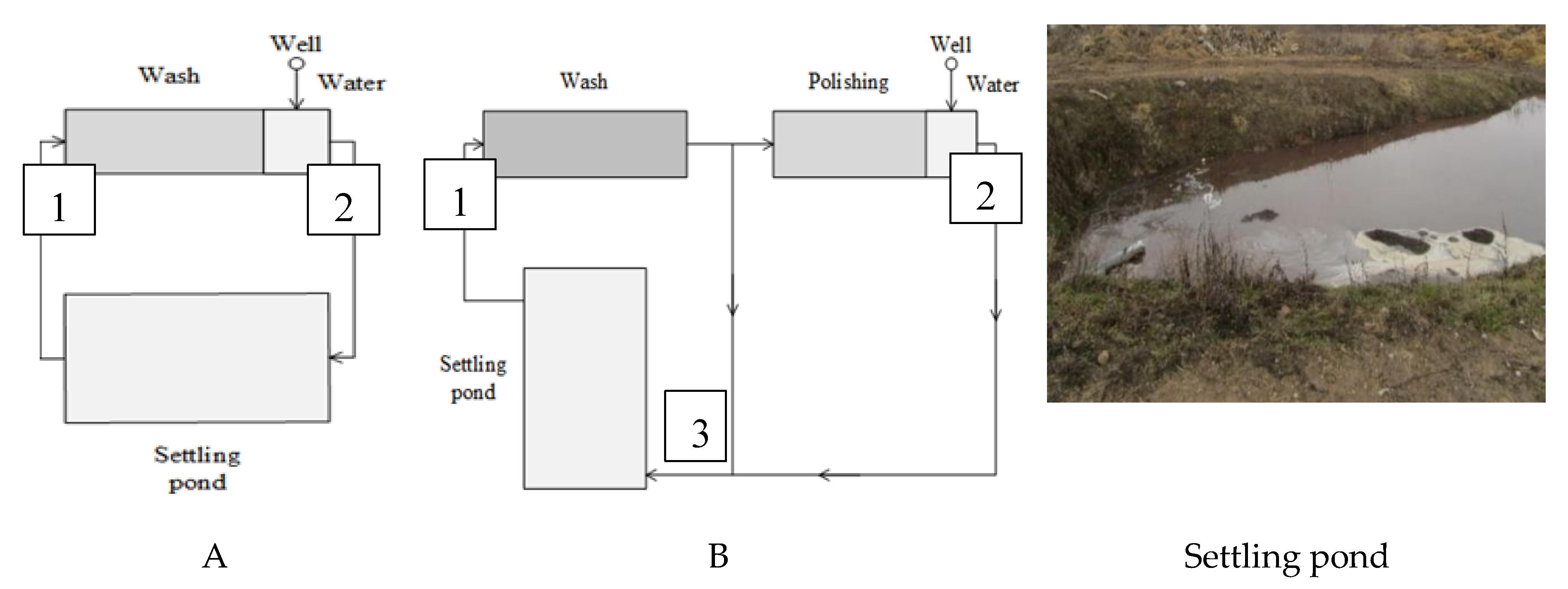
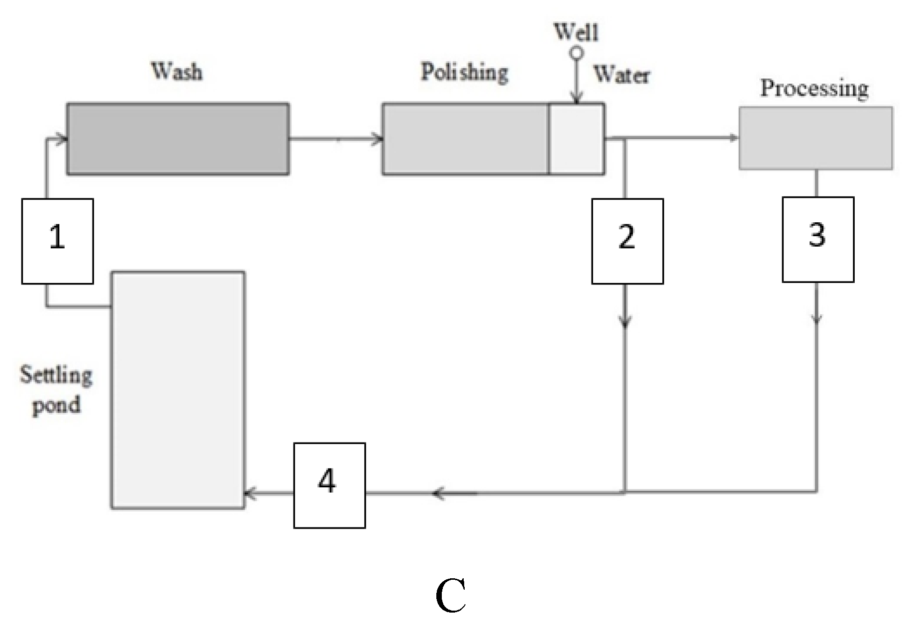
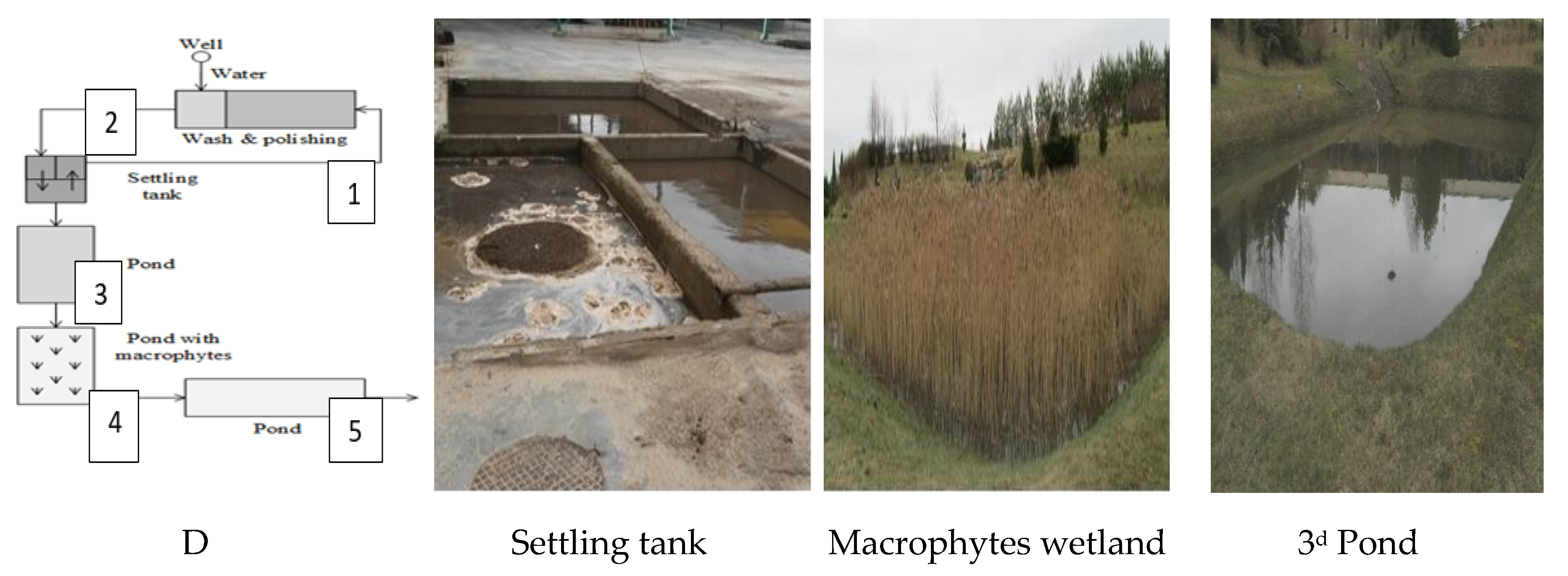
2.1. Description of the Root-Vegetables Washing and Wastewater Treatment Systems

Four typical farms were chosen that represent different root vegetables, such as carrots and beetroots, and use different washing and wastewater treatment systems. All farms transferee the washing water used to the settling ponds (A–C) or settling tank (D). Settled water continuously is used for the first wash. Groundwater from a well (depth 80–150 m) is used for the final wash of vegetables (Figure 1, Figure 2 and Figure 3). As a certain amount of excess water consistently generates, it is stored in the ponds. Excess water and sediments are spread out on the fields periodically according to legislation.

Parameters of the water flow:

A washing system (Figure 1)—beetroots (5 t h⁻¹): 1st wash—recirculating water from settling pond (22 m³ t⁻¹); 2nd wash—groundwater from well (4 m³ t⁻¹). Wastewater—96–120 m³ day⁻¹.

B washing system (Figure 1)—carrots (3 t h⁻¹): 1st wash—recirculating water from settling pond (10 m³ t⁻¹); polishing and 2nd wash—groundwater from well (2 m³ t⁻¹). Wastewater—56 m³ day⁻¹.

C washing system (Figure 2)—carrots (3 t h⁻¹): 1st wash—recirculating water from settling pond (10 m³ t⁻¹); polishing and 2nd wash—groundwater from well (2 m³ t⁻¹). Wastewater—56 m³ day⁻¹.

D washing system (Figure 3)—carrots (10 t h⁻¹): 1st wash—recirculating water from settling pond (70 m³ t⁻¹); polishing and 2nd wash—groundwater from well (7 m³ t⁻¹); excess flow from settling tank is transferred to the constructed system of three biological ponds. Firstly, excess water is discharged to the biological pond. Then it is supplied to surface flow wetland/macrophytes wetland. After that water is discharged into the 3^d pond and, finally, to the river basin (Figure 3).

Quality of the washing water and wastewater were monitored monthly over a 12-month period at the marked points (Figure 1, Figure 2 and Figure 3). Results of the parameters monitored are presented in the same order as samples taken from marked points.

2.2. Sampling and Laboratory Analyses

The results of parameters monitored are presented in the same order as samples taken from marked sampling points (Figure 1, Figure 2 and Figure 3). Temperature (T, °C) was monitored in-situ. In all cases, water samples were collected by the grab method and kept for one day at 4 °C prior to laboratory analyses. The collected samples were analyzed for the water quality parameters, such as color, suspended solids (SS), total dissolved solids (TDS), pH, electrical conductivity (EC), biological oxygen demand in 5 days (BOD₅), chemical oxygen demand (COD_Cr and COD_Mn), dissolved organic carbon (DOC), Kjeldahl nitrogen (N_Kj), total phosphorus P_tot, and inorganic nitrogen N(NH₄-N + NO₂-N + NO₃-N). Deionized water samples were analyzed as standards.

All analytical methods are in accordance with standard methods [27] of the water and wastewater analysis, such as ISO 11923:1997, ASTM D5907—13, ISO 10523:2008, ISO 7888:1985, ISO 5815-1:2003, ISO 5814:2012, ISO 6060:2003, EN 1484:1997; ISO 8245:2000; EN 12260:2003, BS 6068-2.83:2003; ASTM D7573—09, ISO 7887:2011; ISO 6878:2004; ISO 7150-1:1984; ISO 6777:1984; ISO 7890-3:1988 [27]. For the estimation of the uncertainties in the lab analysis, a triplicate analysis was performed, and the mean results, as well as standard deviation, were calculated. Measurements of the UV/Vis absorbance were performed with UV/Vis spectrophotometer Helios γ (Thermo Scientific, USA) in the range of 210 to 660 nm in a quartz cell of 10 mm path length after appropriate dilution with deionised water in order to overcome signal saturation in the UV region (absorbance values above 1 a.u.). In addition, blank samples of deionized water were measured to adjust the 100% transmittance signal. The data set was composed of 672 spectra of washing water and wastewater samples collected over a period of 12 months and of deionized water (control) at specific wavelengths of the UV/Vis spectra. Absorbance at A210 nm is used for roughly evaluation of nitrates, A225 nm—detergents, A240 nm—organic matter OM + suspended solids SS, A254 nm—dissolved organic carbon DOC, A320 nm—suspended solids SS, A390 nm—color, A660 nm—turbidity [2,6,28]. The dissolved organic carbon (DOC) quality was evaluated by specific ultraviolet absorbance (SUVA). SUVA₂₅₄, which indicates the proportion of aromatic compounds in the DOC, was calculated according to equation [29]:

SUVA₂₅₄ (L/mg·M) = A254 (cm⁻¹)/DOC (mg/L)·100 cm/M

(5)

Normally SUVA index of surface waters ranges from 1 to 6. As SUVA index increases, a larger concentration of aromatic compounds are in the solution when SUVA < 3, mainly hydrophilic low molecular weight compounds, are present. When SUVA > 4, organic matter is hydrophobic and high in aromatic compounds. Also, the bigger SUVA index can be resulted by iron, colloidal, or other impurities [7,30,31].

In order to use A254 nm as alternative parameters to estimate BOD₅ and COD, suspended solids have to be removed by filtering with a 0.45 μm pore size membrane filter. However, it is inconvenient, time-consuming and expensive. Chevakidagarn [2] studies of wastewater UV/Vis measurements showed a strong linear correlation between absorbance at A550 and the difference of filtered and non-filtered UV absorbance at A260 nm. Some filtered and unfiltered samples were measured at A240 nm, A320 nm, A254 nm and A660 nm and strong linear relationships were obtained (R² 0.7–0.9). Therefore, measurements of unfiltered samples were made without the interference of suspended solids using the equation:

A254_filtrated = A254_nonfiltrated − A660_nonfiltrated

(6)

Each sample’s UV/Vis spectra were composed of three recorded spectra that were averaged after manual removal of erroneous spectra. Initial data were processed and the data arrangement of the data set was performed using the software Excel 2016 (Microsoft, Redmond, WA, USA).

2.3. Chemometrics Methods

The experimental data set was properly arranged in data matrices and auto-scaled (column mean-centered and scaled) to eliminate offsets and changes in measurement scales. Exploratory analysis of the autoscaled data set was conducted by principal component analysis PCA [22,32,33,34,35,36,37]. The main objectives of the principal component analysis (PCA) are the transformation of the original data’s coordinate system into a more relevant one and reduction of the original system dimension using a limited number of the principal components (PC’s) which reflect the inherent structure of the data [38]. A principal component model approximates a given data matrix as follows [28]:

X (n × p) = T (n × d)·LT (d × p) + E (n × p)

(7)

where n represents the number of objects (samples), p—the number of variables (wavelengths), and d—the number of principal components (PC’s), T—the scores matrix, L—the loadings matrix, LT—the transposed loadings matrix, and E—the residuals matrix.

The number of PC’s was determined by the eigenvalue-one criterion analysis of the covariance matrix, according to which only the PC’s with eigenvalues greater than one are considered relevant. The rotation of the components extracted was converted into six iterations by Varimax method with Kaiser normalization in order to extract optimal amount of PC’s. Tests of PC’s derived were performed by correlation and regression means. Two types of plots were obtained from the application of PCA. Loadings plots which describe and map the relationships between water quality parameters and the extracted principal components, and scores plots, which describe and map the mean samples UV/Vis spectra in the new axes defined by the principal components. One-vector scores plot to interpret the spectral PCA results was performed [28].

Multivariate calibration was performed using principal component regression analysis (PCR). The multiple linear regression (MLR) models assume that in addition to the p independent x-variables, a response variable y is measured, which can be explained as a linear combination of the x-variables. The prediction of the factor of interest y_j can be described as [14]:

$${\mathrm{y}}_{\mathrm{j}}{=\mathrm{b}}_0+{\displaystyle \sum }_{\mathrm{i}=1}^{\mathrm{k}}{\mathrm{b}}_{\mathrm{i}}{\mathrm{x}}_{\mathrm{i}}{+\mathrm{e}}_{\mathrm{i},\mathrm{j}}$$

(8)

where b_i is the computed coefficient, x_i represents the absorbance at each wavelength and e_i,j, is the error.

One drawback of PCA technique is that it captures only the characteristics of the X-vector or predictive variables. No importance is given of each predictive variable relation to the dependent or the target variable. Therefore, it is an unsupervised dimension reduction technique. Partial least square (PLS) allows achieving this balance and providing an alternative approach to PCA technique. Therefore, advanced modeling was performed by partial least square regression (PLS) statistical techniques [13,16,22,32,34,37,39,40]. PLS takes the X-Block (physico-chemical properties) and correlates them with Y-Block (spectral data) information to calculate latent variables (LV) for PLS calibration and prediction models. The calibration model is built by means of PLS, outlier tests and validation procedures to reach both high correlation quality and robustness. The result of the calibration procedure is a recovery function. The recovery function is obtained by plotting the reference measurements (actual targets) vs. the predicted values (estimated targets).

Chemometric models are used to correlate the concentrations of required determinants to spectra. Direct chemometric models are not used in wastewater. This is due to the lack of linear absorbance dependence of a single determinant required by Lambert-Beer law and is related to the parameters used for wastewater analysis. Replacement parameters are commonly used (e.g., COD and TSS), and from the specific properties of wastewater—a strong correlation between different parameters (e.g., COD is strongly correlated with filtered COD and TSS). Therefore, there is a need for intermediate chemometric models. They are based on estimating the calibration parameters from the calibration mixtures. They were using intermediate chemometric models. The validity of the Lambert-Beer law is no longer a prerequisite. Background modeling in the main component becomes feasible. Even systems with highly correlated spectra can also be used for multi-component calibrations [41].

The PLS model used takes into account in particular concentration-spectral dependencies and results in the most robust calibrations today. In the case of multifactorial calibration, the entire spectrum assessment is used. The calibration model is built using PLS, various validation procedures and outlier tests. The aim is to achieve high-quality correlations and quality of the analysis. The spectra and reference measurements must be standardized to perform PLS [41]. The procedure includes multi-factor calibration with PLS, multiple cross-validation and detection and elimination of outliers. The whole procedure is repeated until a good calibration result is obtained. The result of the calibration procedure is a recovery function. The recovery function is obtained by plotting actual cells using reference measurements against detailed cells by predicted values [21,42].

The wide range of wavelengths available allows great flexibility in selecting the best correlating wavelengths for the calibration function. This avoids cross-sensitivity. This is an advantage compared to systems that provide absorption measurements of only one or two wavelengths. The UV/Vis spectrometer provides global calibration for given parameters, but recalibration with local reference samples will improve performance and precision for quantitative measurements. For most cases, the reference data is a critical part of the whole calibration procedure. Therefore, to get good calibration results, it is necessary to guarantee the reference measurements’ quality. They should relate to the reference analysis method, sample identity, sampling randomization, measuring range and sampling errors [42].

Quality assessment of the obtained results was performed by comparison of predicted values versus measured values, both for calibration and validation data sets. Model validation, cross-validation procedures, outlier tests and prediction errors RMSEC and RMSEP were performed to reach both high correlation quality and robustness [13,19,21,32].

Statistical analysis was processed with the software IBM SPSS Statistics 23 and Unscrambler v.9.7 [35,43,44].

3. Results and Discussion

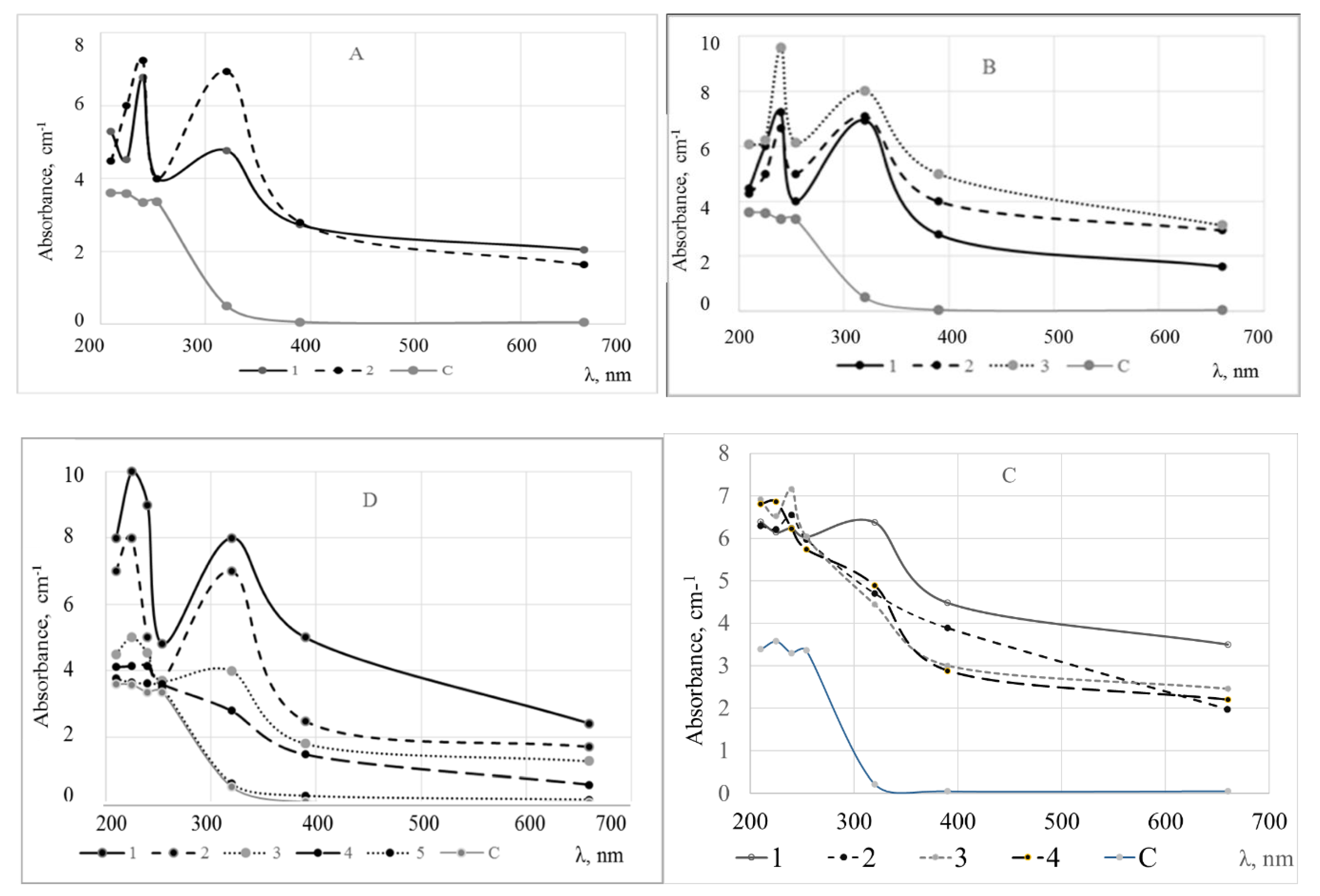
3.1. Data of the Water Quality Monitoring

Descriptive statistics of the physicochemical parameters of the washing water quality are summarized in

Table 1. Descriptive statistics of the washing water physicochemical parameters in the sites monitored and their legislative limits.

Parameter/Sampling Point		SS	TDS	pH	EC	BOD5	CODCr	CODMn	NKj	Nmin	Ptot	DOC	Colour Dilution	SUVA254
		mg L−1	mg L−1		μS cm−1	mgO2 L−1	mgO2 L−1	mgO2 L−1	mg L−1	mg L−1	mg L−1	mg L−1
A	A1 mean	219	1052	7.11	998	221	369	64	22	2.6	3.6	185	7	1.76
N96	A2 mean	987	1419	7.34	969	277	503	178	52	2.5	4.7	217	8	1.84
	Mean	603	1226	7.2	983	261	436	121	23	2.5	4.2	201	8	1.93
	SD	686	748	0.31	171	66	291	81	16	0.1	4	61	4	-
	CV, %	114	61	4	17	24	51	67	70	4	96	27	45	-
	Min	88	371	6.9	805	215	178	64	7	2.4	1	149	3	1.43
	Max	1965	2467	7.6	1214	352	739	178	57	2.7	11	284	12	3.11
B	B1 mean	203	814	6.7	1187	372	403	107	7	nd	1.5	167	6	-
N144	B2 mean	919	1529	7	1027	933	2125	775	17	nd	3.3	332	8	-
	B3 mean	476	800	6.87	1178	445	553	130	7	nd	1.8	153	4	-
	Mean	573	1048	6.9	1127	633	1027	447	12	nd	2	217	6	-
	SD	334	364	2.03	77	306	841	391	9	nd	0.8	83	2	-
	CV, %	58	35	2	7	48	82	87	80	nd	52	38	32	-
	Min	196	786	6.68	1167	297	393	95	2	nd	1	153	4	-
	Max	1089	1715	7.12	1189	119	2125	890	25	nd	4.5	345	8	-
C	C1 mean	470	-	4.6	1146	2718	3229	896	42	nd	13	1125	-	2.52
N192	C2 mean	306	-	4.6	979	2050	2531	568	32	nd	9	764	-	2.34
	C3 mean	9559	-	4.4	-	10,758	20,902	-	357	nd	55	-	-	1.2
	C4 mean	1541	-	4.5	1132	3458	4626	792	53	nd	16	1053	-	2.18
	Mean	5793	-	4.5	1086	7322	13,428	752	222	nd	37	981	-	2.35
	SD	10,304	-	0.15	92	6332	14,911	168	242	nd	30	191	-	-
	CV,%	178	-	3	9	86	111	22	109	nd	81	19	-	-
	Min	274	-	4.2	905	1985	2026	541	27	nd	7	705	-	1.17
	Max	28,490	-	4.65	1165	17,940	41,891	928	580	nd	72	1215	-	2.96
D	D1 mean	3419	884	7.8	726	275	788	-	5	nd	2	279	5	1.95
N240	D2 mean	4834	1200	7.65	720	439	1628	-	15	nd	5	251	6	2.73
	Mean	4362	989	7.7	722	371	1348	-	12	nd	4	260	6	2.79
	SD	2885	184	0.1	22	85	557	-	8	nd	2	25	2	-
	CV,%	66	19	2	3	23	41	-	70	nd	47	9	37	-
	Min	2067	867	7.51	698	254	768	-	4	nd	1	233	4	1.44
	Max	7600	1248	7.83	1214	470	1905	-	21	nd	6	279	8	2.73
	D3 mean	931	683	7.01	715	305	360	-	4	nd	0.4	80	5	2.98
	D4 mean	430	595	7.55	683	156	192	-	3	nd	0.2	82	4	4.57
	D5 mean	4.1	325	8.26	376	7.4	41	-	1.2	nd	0.1	36	1	9.59
	Mean	345	519	7.6	604	57	197	-	3	nd	0.2	68	3	5.66
	SD	486	215	0.56	162	86	132	-	1	nd	0.1	34	2	-
	CV, %	141	42	7.4	27	151	67	-	51	nd	66	49	50	-
	Min	2.4	176	6.98	261	4.5	21.6	-	0.1	nd	0	32	1	2.2
	Max	1543	768	8.46	726	504	375	-	4	nd	0.4	120	7	10.83
Average		2335	946	6.78	904	1729	3287	440	54	2.5	9.8	345	6	3.18
Limits	Canada **	25–40	-	-	-	20–35	-	-	2–8	1–3	0.5–1.0		-	-
	LT ***	-	2000	6.5–8.5	2500	46(29) *	125	-	30	28.5	4	(*) 100–122	3	-
	EU *****	35–60	-	-	-	25	125	-	10–15	-	1–2	-	-	-
HN 24:2003		-	-	6.5–9.5	-	-	-	5	-	51	-	-	-	-

nd—not detected/bellow limit of detection, - no data. * 46—discharge limit per day, 25—disposable discharge limit. ** F-5-1 Determination Of Treatment Requirements For Municipal And Private Sewage Treatment Works; *** Ministry of Environment of the Republic of Lithuania concerning wastewater treatment. https://www.e-tar.lt/portal/lt/legalAct/TAR.4D0DFCDD673A. (*) Calculated from data (Figure 4). ***** Directive 91/271/EEC. Council Directive 91/271/EEC concerning urban wastewater treatment https://eur-lex.europa.eu/legal-content/EN/TXT/?uri=celex%3A31991L0271 HN 24:2003. Drinking water requirements. https://www.e-tar.lt/portal/lt/legalAct/TAR.2099D15473C7.

. Determination of the dissolved organic carbon (DOC) with TOC analyzer is the modern and rapid method. However, limit values of DOC are still under consideration by some researchers [2,5,7,10,30,45]. DOC can also be described by means of COD or BOD₅. Results of this research showed the average fit of the linear regression models (Figure 4).

It can be seen from the model, that the DOC limit values of the root vegetable washing water are in the range between 100 to 122 mg L⁻¹.

Contamination of municipal wastewater depends of its origin and load, particle sizes, rainfalls, storm events, and other conditions [2,3,5,9]. According to the literature suspended solids (SS) of the root vegetables washing water vary within the range 85–930 mg L⁻¹; total dissolved solids (TDS)—425–4650 mg L⁻¹, pH—6.80–11.1, chemical oxygen demand COD mg L⁻¹—160–800 mg L⁻¹, soluble COD—140–350 mg L⁻¹, biological oxygen demand BOD₅—73–1700 mg L⁻¹, SUVA index—1–6, Kjeldahl nitrogen N_Kj—11.4–165 mg L⁻¹, inorganic nitrogen N—2.81–75.5 mg L⁻¹, ammonia NH₃-N—3.8–75 mg L⁻¹,nitrites NO₂-N—<0.005–0.195 mg L⁻¹, nitratesNO₃-N < 0.005–3.17 mg L⁻¹; total phosphorus P_tot—3.0–320 mg L⁻¹ [7,30,31,45,46,47]. Average SS value (2335) in the water samples monitored exceeded common values, COD (440), N_Kj [47], P_tot (9.8), pH (6.78), TDS (946) and SUVA (3.18) values were in the range of the typical wastewater contamination, while N_min (2.5) was slightly lower.

Microbiological contamination (consisted of pathogenic microorganisms Total viable count (TVC) > 300 cfu mL⁻¹), E. coli (5.5 × 10³–1.0 × 10⁴ cfu mL⁻¹), intestinal enterococci (2.8 × 10²–1.5 × 10⁴ cfu mL⁻¹), and coliform bacteria (1.6 × 10³–2.0 × 10⁴ cfu mL⁻¹). Their overall (2 logs/mL) concentration is typical for standing wastewaters [48,49]. As this topic isn’t the focus of this paper, it will not be described further.

Limits of wastewater discharge are based on a condition that no discharge should compromise the current state of a receiving water body [50]. They vary between countries. As shown in Table 1, the average SS concentration exceeded limit values for up to 40–90 times, BOD₅—38–86 times, COD_Cr—26 times, COD_Mn—88 times, N_Kj—1.8, P_tot—2.5–19.6 and color—2 times.

The main reasons for the root vegetables washing water contamination and its’ restriction of possible reuse in the packhouses are suspended solids (SS), biochemical oxygen demand (BOD₅), chemical oxygen demand (COD), Kjeldahl nitrogen N_Kjt and total phosphorus P_tot. Washing water of the carrots is more contaminated than that of beetroots, especially after polishing and processing. These findings show that the root vegetables’ washing water is greatly contaminated and must be treated before discharge or further usage.

SUVA index was in the range of wastewater and natural waters. The third pond of the wastewater treatment system D increased sharply as DOC content was reduced greatly due to sedimentation and microbial decomposition. It is dominated by high molecular weight humic substances as it is typical for natural standing waters [7,30,31,51].

UV/Vis spectra were in accordance with typical absorbance spectra of wastewaters [2,6,28]. Two peaks at A240 and A320 indicate increased amounts of organic compounds and suspended solids. In addition, the effect of wastewater treatment of the pond in system D are obvious. It is obvious that absorbance decreases and the spectra of the water in the sampling spot 5 at the D site are close to the spectra of the deionized water (Figure 5).

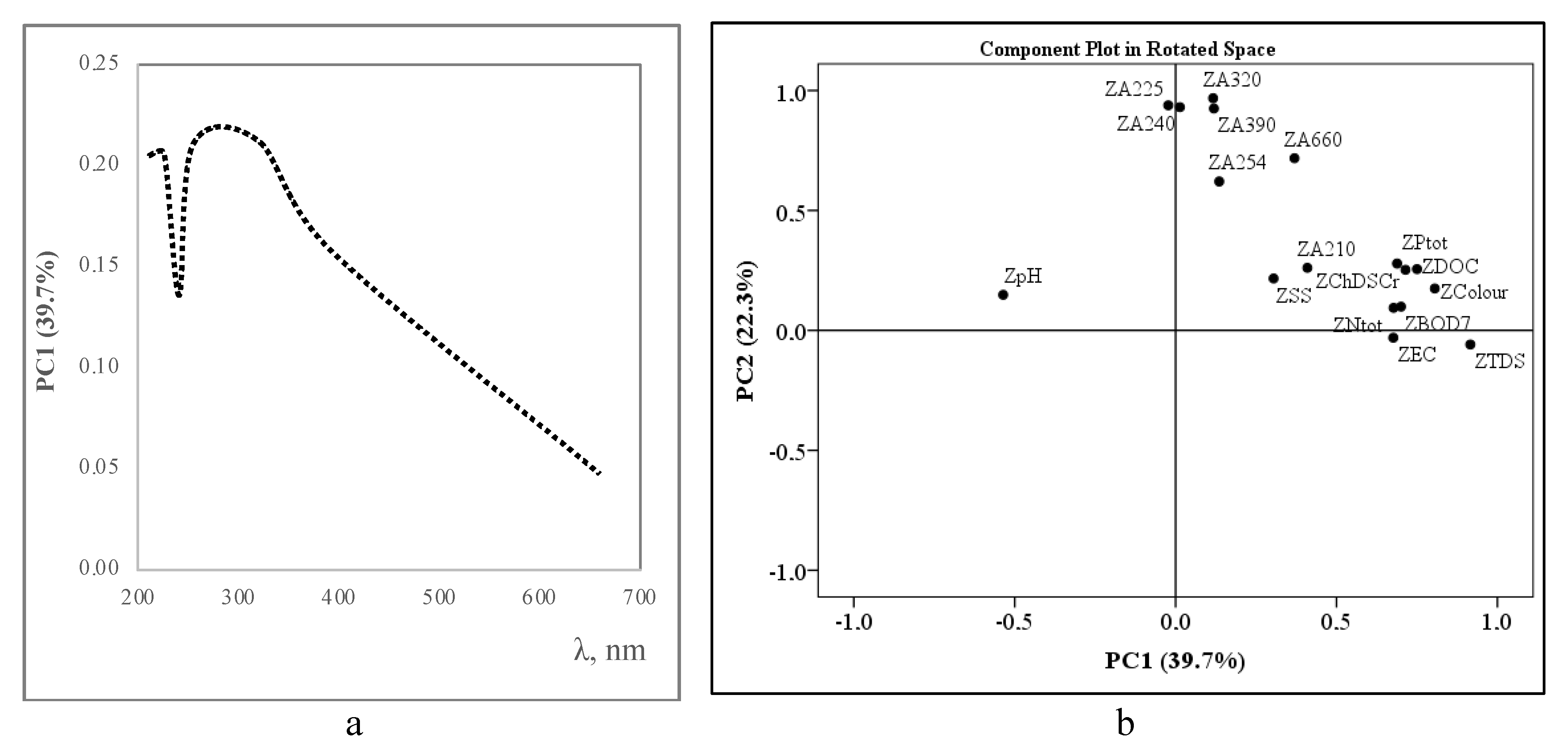
3.2. PCA and PCR Results of the Data Set

In order to prove the hypothesis, factor analysis was performed using the PCA method. Kaiser-Meyer-Olkin measure of sampling adequacy criterion (KMO) was 0.649, a significance level of Bartlett’s test of sphericity Sig. < 0.0001. All measures of sampling adequacy (MSA) were >0.520. Extraction communalities were high and varied from 0.415 to 0.957. This indicates that the extracted components are a good representation of the variables (four extracted PCs explained 80.2% of the total data variance [52]). Principal component PC1 (39.5%) named as “Spectral data” was explained by UV/VIS spectral data excluding absorbance at the wavelength A 210 nm. Principal component PC2 (22.3%) named as “Dissolved solids” is explained by the N_Kj, P_tot, TDS, and color. Principal component PC3 (11.0%) named as “Organic substances” is explained by COD_Cr, BOD₅, and DOC. PC4 (7.5%), named as “Electrochemical properties” is explained by the pH, EC, and A210 nm, which is the measure of nitrates and is related to the electrochemical properties.

Scores plot of the principal component analysis (PCA) for principal component PC1 that describe and map the UV/Vis absorbance data in the new axes defined by the principal components, and loadings plot PC1vs PC2 that describe and map the relationships between water quality parameters and the principal components extracted are shown in Figure 6.

UV/Vis scores plot of spectral data revealed the highest correlation at 270–320 nm showing the highest DOC and SS contribution to PC1 while the lowest correlation was at 240 nm and decreased evenly from 320 nm to 660 nm. These findings confirm some speculations that DOC correlates better with UV/Vis spectra in comparison to organic matter (OM) while SS interferes with them due to scattering [5,21,30]. The right-side variables in Figure 6b are positively correlated one with another and with chemical analytes of the wastewater. Two clusters of the chemical properties and spectral data were established, while pH seems to be an outlier. Significant Pearson correlations (p < 0.05) were observed between PC1 (spectral data), PC3 (organic matter) (r = 0.86) and PC4 (electrochemical properties) (r = −0.79) while the correlation of PC2 (dissolved solids) was wake and statistically insignificant. The Chi-Square test (Asymp. Sig. 0.102 > 0.05) confirmed that our model consisting of four PCs represents a sufficient description of the chemical data. One-Sample Kolmogorov-Smirnov Test (Asymp. Sig < 0.05) confirmed the hypothesis about compatibility between normal empirical and theoretical distributions of PCs. Monte Carlo significance p > 0.05 let to reject H0 hypothesis and conclude that the PCs’ distributions are compatible with normal distribution. Data of the Cook’s test < 4 showed that there are not outliers in the model. Mahalanobis test identified outlier sample only of deionized water, which was used as background for spectral analysis.

Results of the principal components regression (PCR) analysis were unreliable likely due to correlation between dependent variables, so called multi-collinearity (VIF < 2) [38]. The correlation coefficient (R 0.477) and coefficient of determination (R² 0.200) indicate sufficient strength of the linear trend between the variables in the linear regression model according to the equation:

PC UV/Vis = β₀ + β₁ PC Electrochemical + β₂PC Organic matter + β₃PC Dissolved solids + ε

(9)

However, significance levels of the ANOVA (0.273) and coefficients β (0.093; 0.773; 0.229; 0.143) were statistically insignificant (p > 0.05) and model of PCR was unreliable probably because of correlations of many predictors [17,21,43,44]. Therefore, further statistical analysis was performed by partial least square (PLS) model [10,14,34,37,44].

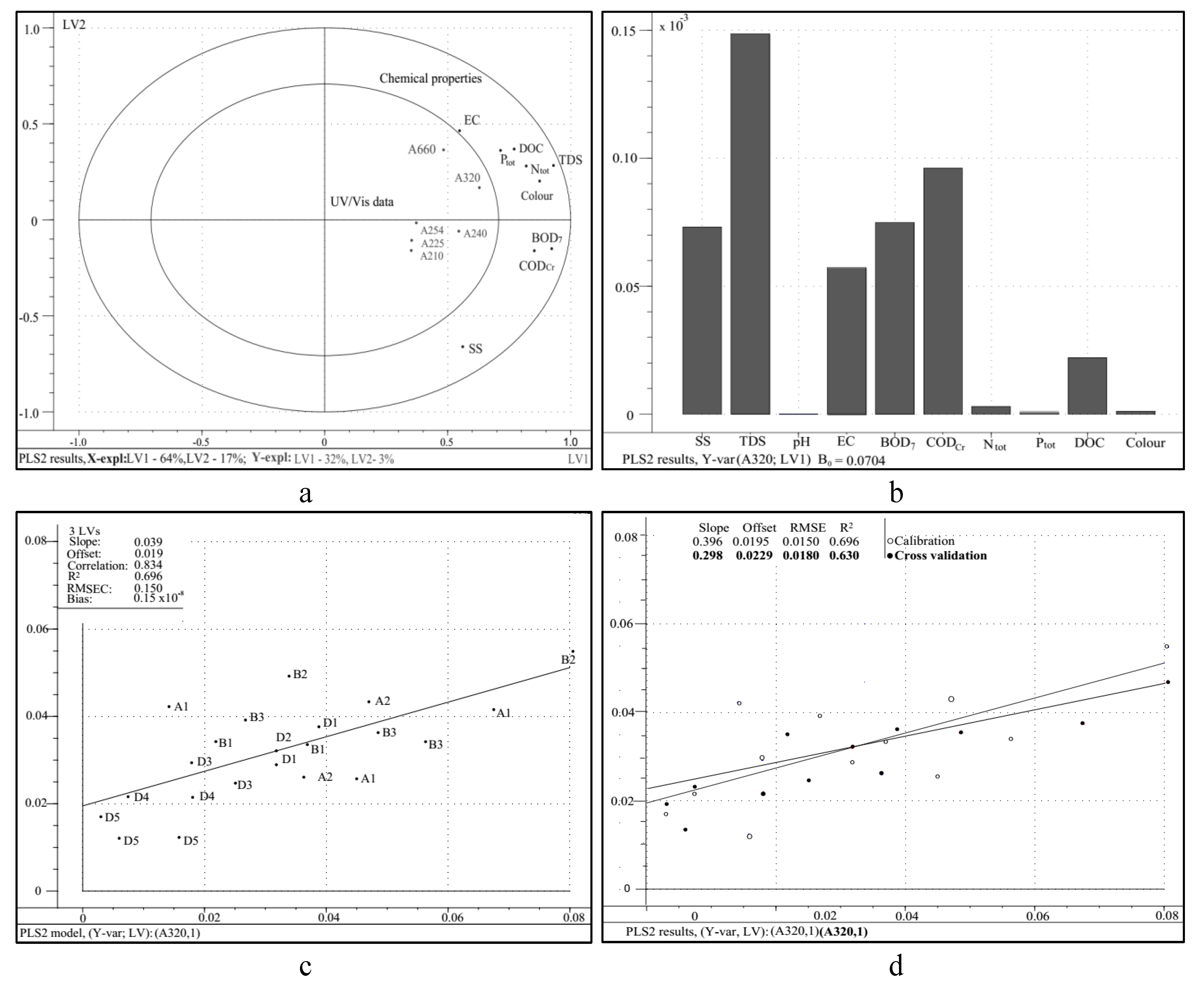
3.3. PLS Regression and Prediction Results of the Data Set

Partial least square regression model (PLS2) of the mean-centered spectral data with three latent variables (LV) explained 85% of the total variance while LV1 explained 32% after calibration, cross-validation, and outliers’ removal. The best fitting to the model showed data at absorbance of A320 (Figure 7).

PLS2 regression model confirmed PCA findings of two uncorrelated clusters (Figure 5b) and showed the great influence of suspended solids (SS), dissolved solids (TDS and EC), and organic matter (BOD₅, COD_Cr, and DOC) while the influence of pH, N_Kj, P_tot and color was negligible. In

Table 2. Limit values of the root vegetables washing water and wastewater chemical contamination (Table 1) and UV/Vis spectra.

	Min	Max	Mean	SD
SS, mg L−1	25.0	60.0	42.5	24.7
TDS, mg L−1	2000	2000	2000	0.00
pH	6.50	9.50	8.00	2.10
EC, µS cm−1	2500	2500	2500	0.00
BOD5, mg L−1	20.0	46.0	33.0	18.4
COD, mg L−1	125	125	125	0.00
DOC, mg L−1	105.0	115.0	110.0	7.10
NKj, mg L−1	2.0	30.0	16.0	19.8
Ptot, mg L−1	0.50	4.00	2.25	2.50
Color, dilution times	3	3	3	0
A210, cm−1	3.997	4.009	4.003	0.008
A225, cm−1	3.886	3.902	3.894	0.011
A240, cm−1	5.193	5.235	5.214	0.030
A254, cm−1	4.042	4.047	4.045	0.004
A320, cm−1	7.387	7.406	7.397	0.013
A660, cm−1	3.946	3.937	3.942	0.006

, the limit values of the contamination of the root vegetables washing water and wastewater and absorbance spectra of the UV/Vis predicted by PLS regression model are presented.

As A320 data have the greatest impact on the model (Figure 5a), it was proposed to use this parameter to monitor water quality in the plants for washing the root vegetables.

4. Conclusions

Chemical analysis of the investigated water samples showed that washing water of root vegetables exceeded the limit values by 10–50 times for suspended solids, 10–25 times for organic matter, 3–5 times for dissolved organic carbon, 3–7 times for total nitrogen, 3–12 times for total phosphorus, and by 3–10 times for microorganisms. Therefore, washing water quality monitoring and proper wastewater treatment is of great importance.

UV/Vis absorbance spectra indicated increased amounts of organic compounds and suspended solids and effects of the water treatment in the ponds system.

PCA and PLS regression methods have been applied to analyze relationships between chemical properties and UV/Vis spectral data. The PCA and PLS modeling results showed that UV/Vis at 320 nm could be a sufficient measure for the water pollution with suspended, dissolved solids and organic matter monitoring. According to these materials’ chemical limit values, limit value of the absorption at A320 nm is 7.39–7.41 cm⁻¹. This limit value will be validated at the feature research.

References

1. Alin, J.; Rubino, M.; Auras, R. Effect of the Solvent on the Size of Clay Nanoparticles in Solution as Determined Using an Ultraviolet-Visible (UV-Vis) Spectroscopy Methodology. Appl. Spectrosc. 2015, 69, 671–678. [Google Scholar] [CrossRef] [PubMed]
2. Chevakidagarn, P. BOD5 Estimation by Using UV Absorption and COD for Rapid Industrial Effluent Monitoring. Environ. Monit. Assess. 2006, 131, 445–450. [Google Scholar] [CrossRef] [PubMed]
3. Jabari, M.; Aqra, F.; Shahin, S.; Khatib, A. Monitoring chromium content in tannery wastewater. J. Argent. Chem. Soc. 2009, 97, 77–87. [Google Scholar]
4. Bakeev, K.A. Process Analytical Technology: Spectroscopic Tools and Implementation Strategies for the Chemical and Pharmaceutical Industries; John Wiley & Sons: Hoboken, NJ, USA, 2010; p. 576. [Google Scholar]
5. Thomas, O.; Jung, A.; Causse, J.; Louyer, M.; Piel, S.; Baures, E.; Thomas, M. Revealing organic carbon–nitrate linear relationship from UV spectra of freshwaters in agricultural environment. Chemosphere 2014, 107, 115–120. [Google Scholar] [CrossRef] [PubMed]
6. Thomas, O.; Burgess, C. (Eds.) UV-Visible Spectrophotometry of Water and Wastewater; Elsevier: Amsterdam, The Netherlands, 2007; 538p. [Google Scholar]
7. Maqbool, T.; Cho, J.; Hur, J. Spectroscopic descriptors for dynamic changes of soluble microbial products from activated sludge at different biomass growth phases under prolonged starvation. Water Res. 2017, 123, 751–760. [Google Scholar] [CrossRef] [PubMed]
8. Langergraber, G.; Fleischmann, N.; Hofstaedter, F.; Weingartner, A.; Lettl, W. Detection of (unusual) changes in wastewater composition using UV/VIS spectroscopy. In Proceedings of the 9th IWA Conference on Design, Operation and Costs of Large Wastewater Treatment Plants, Prague, Czech Republic, 1–4 September 2003. [Google Scholar]
9. Gamerith, V.; Steger, B.; Hochedlinger, M.; Gruber, G. Assessment of UV/VIS-spectrometry performance in combined sewer monitoring under wet weather conditions. In Proceedings of the 12nd International Conference on Urban Drainage, Porto Alegre, Brazil, 11–16 September 2011; Institute of Urban Water Management and Landscape Water Engineering: Graz, Austria, 2011; pp. 1–9. [Google Scholar]
10. Platikanov, S.; Rodriguez-Mozaz, S.; Huerta, B.; Barceló, D.; Cros, J.; Batle, M.; Poch, G.; Tauler, R. Chemometrics quality assessment of wastewater treatment plant effluents using physicochemical parameters and UV absorption measurements. J. Environ. Manag. 2014, 140, 33–44. [Google Scholar] [CrossRef] [PubMed]
11. Workman, J. The Concise Handbook of Analytical Spectroscopy: Theory, Applications, and Reference Materials; Ultraviolet Spectroscopy, Visible Spectroscopy; World Scientific: New Jersey, NJ, USA, 2016; Volumes 1 and 2. [Google Scholar]
12. Geladi, P. Chemometrics in spectroscopy. Spectrochim. Acta Part B At. Spectrosc. 2003, 58, 767–782. [Google Scholar] [CrossRef]
13. Brereton, R.G. Applied Chemometrics for Scientists; John Wiley & Sons: Hoboken, NJ, USA, 2007; 397p. [Google Scholar]
14. Cao, N. Calibration Optimization and Efficiency in Near Infrared Spectroscopy. Ph.D. Thesis, Iowa State University, Ames, IA, USA, 2013; pp. 1–184. [Google Scholar]
15. Chau, F.T.; Liang, Y.Z.; Gao, J.; Shao, X.G. Chemometrics: From Basics to Wavelet Transform; John Wiley & Sons: Hoboken, NJ, USA, 2004; 327p. [Google Scholar]
16. Gemperline, P. Practical Guide to Chemometrics; CRC Press: Boca Raton, FL, USA, 2006; 552p. [Google Scholar]
17. Otto, M. Chemometrics: Statistics and Computer Application in Analytical Chemistry; John Wiley & Sons: Hoboken, NJ, USA, 2007; 328p. [Google Scholar]
18. Kumar, N.; Bansal, A.; Sarma, G.; Rawal, R.K. Chemometrics tools used in analytical chemistry: An overview. Talanta 2014, 123, 186–199. [Google Scholar] [CrossRef]
19. Roussel, S.; Preys, S.; Chauchard, P.; Lallemand, J. Multivariate data analysis (Chemometrics). In Process analytical Technology for the Food Industry; Springer Science: New York, NY, USA, 2014; pp. 7–16. [Google Scholar]
20. Vaillant, S.; Pouet, M.-F.; Thomas, O. Methodology for the characterisation of heterogeneous fractions in wastewater. Talanta 1999, 50, 729–736. [Google Scholar] [CrossRef]
21. Langergraber, G.; Fleischmann, N.; Hofstädter, F. A multivariate calibration procedure for UV/VIS spectrometric quantification of organic matter and nitrate in wastewater. Water Sci. Technol. 2003, 47, 63–71. [Google Scholar] [CrossRef] [Green Version]
22. Miller, J.N.; Miller, J.C. Statistics and Chemometrics for Analytical Chemistry, 6th ed.; Prentice Hall: Harlow, UK, 2010; ISBN 978-0-273-73042-2. [Google Scholar]
23. Aguado, D.; Rosen, C. Multivariate statistical monitoring of continuous wastewater treatment plants. Eng. Appl. Artif. Intell. 2008, 21, 1080–1091. [Google Scholar] [CrossRef]
24. Rieger, L.; Langergraber, G.; Siegrist, H. Uncertainties of spectral in situ measurements in wastewater using different callibration approaches. Water Sci. Technol. 2006, 53, 187–197. [Google Scholar] [CrossRef] [PubMed]
25. Lourenço, N.D.; Menezes, J.C.; Pinheiro, H.M.; Diniz, D. Development of PLS calibration models from uv-vis spectra for TOC estimation at the outlet of a fuel park wastewater treatment plant. Environ. Technol. 2008, 29, 891–898. [Google Scholar] [CrossRef] [PubMed]
26. Brito, R.S.; Pinheiro, H.; Ferreira, F.D.R.; Matos, J.S.; Lourenço, N. In situUV-Vis spectroscopy to estimate COD and TSS in wastewater drainage systems. Urban Water J. 2013, 11, 261–273. [Google Scholar] [CrossRef]
27. Standard Methods. Standard Methods for the Examination of Water and Wastewater, 22nd ed.; American Public Health Association/American Water Works Association/Water Environment Federation: Washington, DC, USA, 2012. [Google Scholar]
28. Lourenço, N.D.; Chaves, C.; Novais, J.; Menezes, J.C.; Pinheiro, H.; Diniz, D. UV spectra analysis for water quality monitoring in a fuel park wastewater treatment plant. Chemosphere 2006, 65, 786–791. [Google Scholar] [CrossRef]
29. Potter, B.B.; Wimsatt, J.C. Method 415.3—Measurement of Total Organic Carbon, Dissolved Organic Carbon and Specific UV Absorbance at 254 nm in Source Water and Drinking Water; U.S. Environmental Protection Agency: Washington, DC, USA, 2005; 53p.
30. Korshin, G.V.; Chow, C.W.; Fabris, R.; Drikas, M. Absorbance spectroscopy-based examination of effects of coagulation on the reactivity of fractions of natural organic matter with varying apparent molecular weights. Water Res. 2009, 43, 1541–1548. [Google Scholar] [CrossRef]
31. Vepsäläinen, M.; Sillanpää, M. Electrocoagulation in The Treatment of Industrial Waters and Wastewaters; Elsevier: Amsterdam, The Netherlands, 2020; Volume 19, pp. 1–78. [Google Scholar]
32. Esbensen, K.H.; Guyot, D.; Westad, F.; Houmoller, L.P. Multivariate Data Analysis: In Practice, 5th ed.; CAMO Process AS: Oslo, Norway, 2002; 598p. [Google Scholar]
33. Intelligent Data Analysis: An Introduction. Technometrics 2005, 47, 104. [CrossRef]
34. Abdi, H.; Williams, L.J. Partial Least Squares Methods: Partial Least Squares Correlation and Partial Least Square Regression. In Bioinformatics in MicroRNA Research; Springer Science and Business Media LLC: Berlin, Germany, 2013; Volume 930, pp. 549–579. [Google Scholar]
35. Garson, G.D. Factor Analysis; Statistical Associates Publishers: Asheboro, NC, USA, 2013; p. 131. [Google Scholar]
36. Jolliffe, I.T. Principal Component Analysis; Springer: Berlin, Germany, 2013; 271p. [Google Scholar]
37. Dunn, K. Process Improvement Using Data. 2016. Available online: https://learnche.org/pid/# (accessed on 20 October 2020).
38. Maitra, S.; Yan, J. Principle Component Analysis and Partial Least Squares: Two Dimension Reduction Techniques for Regression; Casualty Actuarial Society Discussion Paper Program: Arlington, VA, USA, 2008; pp. 79–90. Available online: http://www.casact.org/pubs/dpp/dpp08/08dpp76.pdf (accessed on 20 October 2020).
39. Wold, S.; Sjostrom, M.; Eriksson, L. PLS-regression: A basic tool of chemometrics. Chemom. Intell. Lab. Syst. 2008, 58, 109–130. [Google Scholar] [CrossRef]
40. Brown, S.D. Book Reviews: Introduction to Multivariate Statistical Analysis in Chemometrics. Appl. Spectrosc. 2010, 64, 112A. [Google Scholar] [CrossRef]
41. Otto, M. Chemometrics: Statistics and Computer Application in Analytical Chemistry; John Wiley & Sons: Hoboken, NJ, USA, 2016. [Google Scholar]
42. Langergraber, G.; Fleischmann, N.; Hofstaedter, F.; Weingartner, A. Monitoring of a paper mill wastewater treatment plant using UV/VIS spectroscopy. Water Sci. Technol. 2004, 49, 9–14. [Google Scholar] [CrossRef]
43. Garson, G.D. Partial Least Squares: Regression and Structural Equation Models; Statistical Associates Publishers: Asheboro, NC, USA, 2016; 262p. [Google Scholar]
44. CAMO. CAMO Software AS. Unscrambler. 2018. Available online: http://www.camo.com/rt/Products/Unscrambler/unscrambler.html (accessed on 20 October 2020).
45. Orhon, D.; Ates, E.; Sözen, S.; Cokgor, E.U. Characterization and COD fractionation of domestic wastewaters. Environ. Pollut. 1997, 95, 191–204. [Google Scholar] [CrossRef]
46. Tchobanoglous, G.; Burton, F.L.; Stensel, H.D.; Burton, F. Wastewater Engineering: Treatment and Reuse; McGraw-Hill Education; Metcalf & Eddy, Inc.: New York, NY, USA, 2003. [Google Scholar]
47. Henze, M.; Comeau, Y. Wastewater Characterization. In Biological Wastewater Treatment: Principles Modelling and Design; Henze, M., Mark, C.M.v.L., Ekama, G.A., Brdjanovic, D., Eds.; IWA Publishing: London, UK, 2008; pp. 33–53. [Google Scholar]
48. Sežun, M.; Kosel, J.; Zupanc, M.; Hočevar, M.; Vrtovšek, J.; Petkovšek, M.; Dular, M. Cavitation as a Potential Technology for Wastewater Management—An Example of Enhanced Nutrient Release from Secondary Pulp and Paper Mill Sludge. J. Mech. Eng. 2019, 65, 641–649. [Google Scholar] [CrossRef] [Green Version]
49. Sas, W.; Dzięcioł, J.; Głuchowski, A. Estimation of Recycled Concrete Aggregate’s Water Permeability Coefficient as Earth Construction Material with the Application of an Analytical Method. Materials 2019, 12, 2920. [Google Scholar] [CrossRef] [PubMed] [Green Version]
50. Rozema, E. Water Quality Parameters and Discharge Limits. In HMGA Water Project; HMGA Water Project: Bradford, ON, Canada, 2016; Available online: http://www.hmgawater.ca/ (accessed on 20 October 2020).
51. Kosel, J.; Šuštaršič, M.; Petkovšek, M.; Zupanc, M.; Sežun, M.; Dular, M. Application of (super)cavitation for the recycling of process waters in paper producing industry. Ultrason. Sonochem. 2020, 64, 105002. [Google Scholar] [CrossRef] [PubMed]
52. Keho, Y. The Basics of Linear Principal Components Analysis. In Principal Component Analysis; Intech: London, UK, 2012; pp. 181–207. [Google Scholar]
Figure 1. Flowchart of root vegetable washing systems: A—beetroots, B—carrots and view of settling pond.
Applsci 10 09072 g001
Figure 2. Flowchart of carrots washing and processing system C.
Applsci 10 09072 g002
Figure 3. Flowchart and view of the carrots washing and wastewater treatment system D.
Applsci 10 09072 g003
Figure 4. Linear regression models of the BOD and COD to DOC.
Applsci 10 09072 g004
Figure 5. UV/VIS fingerprints of the washing water and wastewater monitored at the sampling spots 1, 2, 3, 4 and 5 (Figure 1, Figure 2 and Figure 3), C—deionized water.
Applsci 10 09072 g005
Figure 6. PCA scores plot of the UV/Vis absorbance for PC1 (a) and PC1 vs. PV2 (b) loadings plot of the water quality parameters monitored.
Applsci 10 09072 g006
Figure 7. PLS regression model overview plot: (a)—correlation loadings between chemical properties (x variables) and UV/Vis spectra (y variables); (b)—the importance of the chemical properties (x variables) on the model, (c)—model calibration, (d)—model validation for A320.
Applsci 10 09072 g007