Abstract
In the rehabilitation field, clinicians are continually struggling to assess improvements in patients following interventions. In this paper, we propose an approach to use gait analysis based on inertial motion capture (MoCap) to monitor individuals during rehabilitation. Gait is a cyclical movement that generates a sufficiently large data sample in each capture session to statistically compare two different sessions from a single patient. Using this crucial idea, 21 heterogeneous patients with hemiplegic spasticity were assessed using gait analysis before and after receiving treatment with botulinum toxin injections. Afterwards, the two sessions for each patient were compared using the magnitude-based decision statistical method. Due to the challenge of classifying changes in gait variables such as improvements or impairments, assessing each patient’s progress required an interpretative process. After completing this process, we determined that 10 patients showed overall improvement, five patients showed overall impairment, and six patients did not show any overall change. Finally, the interpretation process was summarized by developing guidelines to aid in future assessments. In this manner, our approach provides graphical information about the patients’ progress to assess improvement following intervention and to support decision-making. This research contributes to integrating MoCap-based gait analysis into rehabilitation.
1. Introduction
In the field of rehabilitation, clinicians continuously assess the improvement of patients to verify that treatments or therapies are achieving satisfactory results. In this context, numerous treatments are aimed at improving the ability to walk because this activity is essential to quality of life and personal autonomy. One clear example of this is the importance of rehabilitation treatments in the recovery of an individual with hemiplegic spasticity following a stroke who experiences walking impairment [1,2,3,4,5,6].
Currently, assessing gait improvements after treatment is normally conducted through qualitative techniques, either by observation or through interviews with the patient [7]. However, these existing techniques could incorporate technology providing objective information regarding the patient’s progress without requiring excessive time or advanced technological knowledge on the part of clinicians.
In this regard, gait analysis based on motion capture (MoCap) involves the measurement, analysis, and interpretation of human locomotion [8]. In the rehabilitation field, the information this analysis provides offers a wide variety of applications, including supporting decision-making for treatments and interventions [9,10,11,12,13,14]. It can support decisions regarding changing; adjusting (e.g., dosage) or discontinuing treatment [15]. Among the existing MoCap technologies, those based on inertial measurement units (IMUs) have been gaining particular relevance because they do not require external cameras and can be embedded into wearable technology [16,17].
Marin et al. [7] demonstrated that it is possible to integrate an IMU gait analysis test into a rehabilitation service such as a medical test. In the same manner, Marin et al. [17] proposed a gait analysis system based on IMUs free of magnetic disturbances, overcoming a limitation of this technology. Additionally, they demonstrated that this technology was reproducible and that the duration of the gait test was compatible with the daily practice of a rehabilitation service.
However, despite the great utility of clinical gait analysis [15,18] and the described advances, for its complete integration into the clinical setting, this technology must still overcome various challenges. One of these is the data analysis resulting from measuring an individual’s gait. Methods must be developed to automatically and repeatedly process the generated spatiotemporal and kinematic variables [8]. More specifically, it is necessary to standardize methods in order to compare the variables generated in two different measurement sessions, between which the patient may have changed his or her gait pattern. For example, this could happen before and after a treatment or intervention or at the beginning of and during the rehabilitation process. Since this comparison of individual gait analysis data is not yet standardized or automated, the time required for data processing, the need for highly qualified professionals to interpret the results, and the handling of massive amounts of data hinder the use of gait analysis as standard practice [8,11,16,19,20].
The comparison of gait variables from two different measurement sessions has been executed among groups of patients in clinical trials studies. Such studies are widespread in clinical research, and many of them have used gait analysis for this purpose [21,22,23,24]. This type of study selects a homogeneous group of patients with a specific pathology and applies a pre- and post-treatment gait test to compare the results between both measurements.
However, this study did not focus on assessing a group of patients. Instead, we deal with the heterogeneity among rehabilitation patients in daily clinical practice. We face the challenge of assessing each patient, comparing the data in one session with the corresponding data of the patient in another session. Concerning this issue, little research has been conducted in biomedical studies [18].
In this regard, gait is a cyclical movement that generates a sufficiently large data sample in each capture session to statistically compare two different sessions (i.e., pre-treatment and post-treatment sessions) from a single patient. Using this essential feature, this paper illustrates how to assess individuals undergoing rehabilitation using the MoCap gait analysis based on IMUs. For this purpose, 21 heterogeneous patients with hemiplegic spasticity were assessed before and after treatment with botulinum toxin injections. To make the statistical comparisons between the two sessions, we used the magnitude-based decision (MBD) method [25]. The information that these comparatives provide can be useful in understanding the evolution of a patient between the two stages, but due to the challenge of classifying changes in gait variables as improvements or impairments, it requires clinical interpretation. Thus, using the information from the 21 individual assessments, we classified the patients according to their overall progress. As a result of this process, we propose interpretation guidelines to improve the applicability of this type of analysis in the clinical environment. This paper seeks to contribute to a data management option for gait analysis that could enhance the integration of MoCap-based gait analysis into rehabilitation.
2. Materials and Methods
2.1. Study Design
Twenty-one patients with hemiplegic spasticity in their lower limbs underwent two MoCap gait tests; the first took place a few minutes before treatment with botulinum toxin (pre-treatment), and the second took place approximately one month later (post-treatment).
In the pre- and post-treatment measurement sessions, we instrumented the patient as shown in Figure 1. Afterwards, he or she walked naturally for six meters in a straight line at a self-selected speed and then turned around and walked back to the starting position multiple times. As we studied the gait cycle, only strides in a straight line were considered for analysis, and turns, starts, and stops were excluded. We measured 25 strides per patient per session.
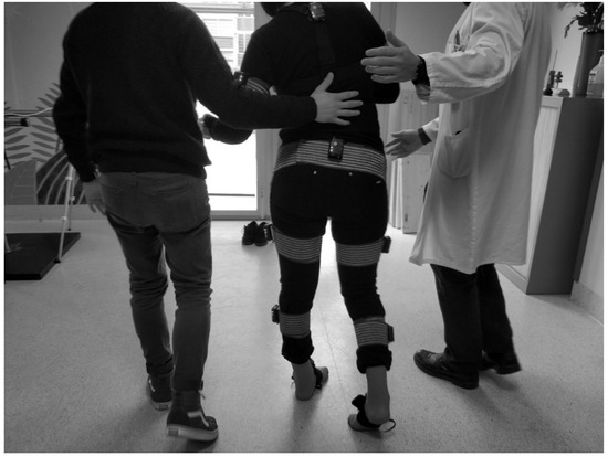
Figure 1.
Gait test in hospital. The sensor placement is shown on a patient with spasticity.
2.2. Ethical Statement
The study was conducted in accordance with the Declaration of Helsinki, and the protocol was approved by the Bioethics Committee of Aragón, Spain (N° 12/2018). A written informed consent was obtained from each participant.
2.3. Technology and Instrumentation
We used the Move Human Sensors MoCap system developed by the IDERGO Research Group, selecting the system’s MH-IMU configuration, which was recently described and assessed by Marin et al. [17]. This system is based on next-generation IMU (NGIMU) devices [26], which measure the rotations via signal processing in embedded sensors (accelerometers, gyroscopes, and magnetometers) and are placed on the body with elastic bands. In our experiment, we used the information from eight IMUs configured at 60 Hz (placed on the feet, calves, thighs, pelvis, and chest) to analyze the gait, as Marin et al. [17] described. Nevertheless, we placed the full-body configuration (15 IMUs) on the participant for possible further investigation. This system incorporates an anatomical calibration procedure that allows for the deactivation of the IMUs’ magnetometers, avoiding the adverse effects that disturbances in the magnetic field may cause. These magnetic disturbances are expected when the participant moves along a few meters especially in a hospital environment, which is filled with different equipment, wiring, and electromagnetic signals. Beyond this, the Move Human Sensors MoCap system includes an algorithm that detects gait events from kinematic data without additional instrumentation. These features justified the selection of this system and may favor the applicability of this technology in the clinical environment.
2.4. Participants
The choice of neurological patients with hemiplegic spasticity provides a challenging environment that enables the extrapolation of the results and methods to other patients with less severe physical or cognitive conditions. Spasticity is a symptom that affects numerous patients. Its adverse effects include pain, decreased mobility, contractures, and muscle spasms, which can interfere with daily activities and sleep to a greater or lesser degree [27,28,29]. In this regard, the botulinum toxin treats focal spasticity via muscle injection with a reversible paralytic action [27,30,31]. Although other treatments for spasticity exist, the observed efficacy; required personalization for each patient (dose, muscles to be inoculated, etc.); and widespread use justify the choice in this study.
We analyzed 21 heterogeneous patients (shown in Table 1), 11 women and 10 men (46 ± 16 y, mean ± SD). They met the general inclusion criterion, which was that the disease allowed them to walk autonomously. The sample of participants corresponds with the circumstances of patients who receive rehabilitation services from public hospitals.

Table 1.
Patient characteristics.
2.5. Variables
We obtained the spatiotemporal and kinematic variables [8,32] shown in Table 2. Each variable, except for GaitSpeed, was calculated for the pathological or affected side (A) and the non-affected or healthy side (H).
Table 2.
Variables considered in the study.
2.6. Magnitude-Based Decision (MBD) to Monitor Individuals with Gait Analysis
Concerning individual monitoring, the human gait is a repetitive cyclical movement; thus, in a measurement session, a variable produces a multitude of samples (e.g., 25 samples of the StepLght variable for Patient S001 in a measurement session). Therefore, to monitor an individual, it is possible to compare two groups of measurements, namely the group of measurements from a pre-treatment session (n1 samples, X1 mean, and SD1 standard deviation) and the group of measurements from a post-treatment session (n2 samples, X2 mean, and SD2 standard deviation). Thus, according to traditional statistical theory, this approach is a two-mean comparison of independent samples because gait cycles, despite being obtained from the same patient, are not pair related.
Regarding the sample of strides recorded in each session, more strides would obviously provide better statistical normality and better precision. However, it was necessary to balance the number of steps to be recorded, the time that the test would take in the daily clinic, and the fatigue that the test could cause in certain patients if they walked for a long time. Thus, we decided to record 25 strides per patient per session. We did this to satisfy the central limit theorem and especially because Kribus-Shmiel et al. [33] ensured that 23 strides usually achieve statistical normality and stability. As will be explained later in this sub-section, to prove that the stride sample was sufficient, we calculated the power of each statistical comparison.
To conduct the comparison between the pre- and post-sessions, applying a student’s t-test of the independent samples to each specific variable could be valid. Applying this test, a p-value lower than 0.05 would indicate that a difference existed between the pre- and pot-sessions. Nevertheless, as Amrhein et al. [34] stated, although it is currently accepted that an effect is significant if the p-value does not exceed a value of 0.05, this generates a dichotomy that is far from reality. According to the Nature Research Journal this statement about the p-value has been supported by more than 800 researchers [34]. Thus, to infer a conclusion, researchers must delve deeper into the results. For this purpose, the magnitude-based inference method, which has recently been rebranded as the MBD method, addresses this need by using a more realistic threshold than a p-value of 0.05. Information about the MBD approach can be found in Excel spreadsheets, presentations, notes, and articles, all of which are available from sportsci.org [35]. The MBD method provides the probability that a change (defined by the confidence interval of the difference, CIdif) exceeds a specific threshold (−δ, +δ) selected by researchers in accordance with their objectives [36,37].
This method is not exempt from controversy; thus, some authors support [38,39,40,41] and others oppose [42,43] its application. However, we assumed this method to transmit a simple and interesting idea, considering a change ‘relevant’ if it exceeds a specific threshold. This idea may not be applicable in all fields but it makes sense in individual patient monitoring. The MBD method has, for example, been applied to elite athletes (e.g., [44]). We found similarities between elite athletes and the patients with spasticity because, in both cases, an individualized evaluation is required due to the uniqueness or heterogeneity of each participant, and it is difficult to compare a participant with a reference database. This idea has also been illustrated by de la Torre et al. [45], who applied MBD to the individual evaluation of patients with vertiginous pathologies.
Therefore, the application of the MBD method requires facing the challenge of establishing an adequate threshold δ. According to the MBD basis, the ideal or optimal solution would be to use as the threshold δ the minimal important difference (MID) [46], the smallest worthwhile change [47], the smallest clinically important value [37], or any other combination of the terms used in the literature to identify changes that have clinical or practical relevance (i.e., changes that have an effect on quality of life). Nevertheless, to the best of our knowledge, no one has proposed MID indexes for gait variables resulting from a MoCap system for the same population or treatment. This would be a challenge requiring in-depth further research beyond the scope of this study.
Thus, until further research provides these MID values, it will be reasonable to affirm that a change is significant if it overcomes at least the errors inherent in the test. In this regard, it will not be known if a change influenced a participant’s quality of life, but at least, it will be known that the change existed and was not the result of a measurement error. This conclusion could be useful for clinicians, especially if they combine it with the rest of the clinical information.
In this regard, Marin et al. [17] recently summarized the error sources of a gait analysis test in the following groups: participant intrinsic variation, soft tissue movement, relative movement between the device and skin, positioning, instrument accuracy, gait event detection, and anatomical calibration. As shown in other studies [2,48,49,50], the magnitude of these errors in our experiment could be estimated for each participant using Bland and Altman’s limits of agreement [51] (see Equation (1)). Using these errors as threshold δ, the MBD method provides the probability that a change had been more than zero. This is the probability that a patient had undergone ‘real’ changes. Reflections about the implication of using this threshold δ will be explored in the Discussion section. In this manner, the threshold δ was calculated using Equation (1):
where Z1−α/2 is the value of the normal distribution at 1 − α/2 (as we stabilized a confidence level of 95%, α was 0.05 and the Z1−α/2 value was 1.96), accounts for errors between two measurements [51,52,53,54], SEdif is the standard error of the difference between the means, n1 and n2 are the respective samples of the pre- and post-tests, and SD1 and SD2 are the respective standard deviations of the pre- and post-tests.
Moving from the threshold δ, another important issue in individualized gait analysis monitoring is that most of the changes in gait variables are not clearly either beneficial or harmful (see the terminology used by Hopkins and Batterham [55]). An increment or decrement in the magnitude of a specific gait variable could be beneficial for one patient but harmful for another. Spasticity causes such alterations to gait that, even if a particular gait variable changes to a value closer to normal, this will not necessarily indicate a beneficial change. In the rehabilitation process of patients with spasticity, the goal is usually to develop, learn, or internalize a gait pattern that is as functional and harmless as possible considering anthropometric, muscular, or cognitive conditions, regardless of the normality of the pattern itself [7,56,57,58]. Therefore, in an experiment like this one, it is necessary to interpret the results for each patient independently.
For this reason, we used the ‘real’ changes provided by the MBD method to conduct a process that we called biomechanical interpretation. Three researchers—J.M. (an engineer), I.S. (a medical doctor), and E.M. (a medical doctor)—independently studied the same results (tables and graphs). They only considered changes that were at least ‘very likely’ (>95% chance). Following a discussion of their reflections and once a consensus had been reached, the conclusions for each patient were listed in detail (see the Supplementary Materials). These researchers later classified the patients into the following three groups: patients with overall improvement, those with overall impairment, and those without overall change. Finally, based on the information acquired during the interpretation process, the researchers wrote interpretation guidelines applicable to other assessments (see Section 4).
After outlining the decisions made in this study regarding the threshold δ and the interpretations of the results, we will introduce how we compared the two groups of measurements using the MBD approach. Hopkins [59] developed a spreadsheet to compare ‘means of two groups’. Based on this spreadsheet, we developed a script applying the MBD method by using as input the threshold δ selected by the researcher, and the measurements taken from the pre- and post-tests of one specific patient. This script was developed using Vizard (6.2 version, WorldViz, Santa Barbara, CA, USA, 2020), which is based on Python 2.7, and the Pandas and Matplotlib libraries. The sequence that this program follows for a two-mean comparison begins with the calculation of the interval of the difference CIdif, which defines the lower and upper limits (Li, Ls) of the change (Equation (2)) [59]:
In Equation (2), tα,DoF is the value of the t distribution for a specific α selected by the researchers, (we defined α as 0.05 to achieve a confidence level of 95%) and a specific degree of freedom (DoF), which is computed with Equation (3) using Welch–Satterthwaite’s approximation [60], where n and SD are the stride sample size and standard deviation, respectively; SEdif is calculated as explained with Equation (1); and the difference between means (Xdif) is computed with Equation (4), where X2 is the post-test mean, and X1 is the pre-test mean.
Exposed calculations assume independent samples, non-equal variances, and data that have approximately normal distribution. This data normality assumption is based on work by Kribus-Shmiel et al. [33], who ensured that statistical stability and normality could be achieved with 23 strides or more and that this number of cycles was sufficient to represent the mean behavior.
After δ and CIdif have been defined, it is possible to develop a graph for each variable, such as the one in Figure 2, representing the threshold (−δ, +δ) and the t-distribution of the change between the pre- and post-series. This representation facilitates analysis where the change falls in relation to the threshold δ. To accomplish this analysis numerically, the percentage of the t area that falls within the ‘negative’ region (−∞, −δ), within the ‘trivial’ region (−δ, +δ), and within a ‘positive’ region (+δ, +∞) must be computed. These areas are respectively labelled as follows: probabilities of negative change (N), trivial change (T), and positive change (P) [37].

Figure 2.
Representation of the change between the pre- and post-series of one variable; δ: magnitude-based decisions (MBD) threshold. Xdif: change within a subject (difference of means between pre- and post-series). Li: lower limit of the change. Ls: upper limit of the change. Note: δ, Xdif, Li, and Ls were computed using Equations (1)–(4).
In this manner, if the percentages of P and N are both less than 5%, (N < 5% and P < 5%), the change is considered null or trivial because it does not exceed the threshold δ in any direction. If P and N are both higher than 5% (N > 5% and P > 5%), the change is categorized as unclear because it simultaneously exceeds the threshold δ in both directions. Any other disposal of CIdif can be categorized as positive (increment) or negative (decrement) with a determined probability of change. If the change is an increment, the probability of change is P, and if the change is a decrement, the probability of change is N. The probability of change is classified as follows: 5 to 25% is ‘unlikely’, 25 to 75% is ‘possibly’, 75 to 95% is ‘likely’, 95 to 99% is ‘very likely’, and greater than 99% is ‘most likely’ [37,61].
Equations (5)–(9) show how to calculate N, T, and P using Excel formulas [59]. These expressions include values computed using the previous equations. Additionally, the choice of the formula used to compute N, T, and P depends on where the Xdif falls in relation to the threshold (−δ, +δ):
The last step of our analysis was to examine whether the sample size of 25 strides was adequate. As described at the beginning of this subsection, we decided to capture 25 strides per patient per session because this number of strides seemed to be adequate according to the literature and provided a reasonable test duration. In this sense, Equation (10) relates the sample size (n) of strides (i.e., 25) to the threshold δ described; the statistical power (1 − β), which is the probability of detecting effects without committing Type II errors (false negatives); the α selected, which is the probability of committing Type I errors (false positive); and the SDpool, which is the pooled standard deviation of the pre- and post-tests:
Equation (10) is a formula based on the normal distribution and is applied for the two mean comparisons [62]. In this equation, Z1−α/2 is the value of the normal distribution at 1-α/2 (as we stabilized a confidence level of 95%, α was 0.05, and the Z1−α/2 value was 1.96), and Z1−β is the value of the normal distribution at 1 − β (e.g., for a power of 80%, the Z1−β value would be 0.84).
Using this equation, we first calculated the power for each statistical comparison using the sample of 25 strides for each variable, patient, and session. Second, from another perspective, we calculated the sample size (n) needed if we fixed the power at 80%, which is the typical stabilized power in research.
3. Results
The results of this study involved 21 separate patient-level analyses. After the interpretation of the MBD results of all the individual patients, it can be said that 10 patients showed overall improvement, five patients showed overall impairment, and six patients did not show overall change. In this section, we present one example of the patient-level analysis (Patient S014) in Table 3 and Figure 3. The numerical results and biomechanical interpretation of all participants are presented as Supplementary Materials in an Excel file.
Table 3.
Results of one patient-level study, patient S014.
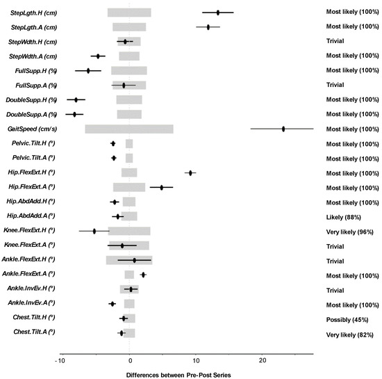
Figure 3.
Patient-level analysis and confidence interval representation for Patient S014. Wide light grey bars: MBD threshold. Thin black bars: Confidence interval of the difference (CIdif).
Note that the N, T, and P terms shown in Table 3 were the result of the statistical comparison using the MBD approach, and their meanings were included in Figure 2 and the related paragraphs in the previous section.
Table 3 includes the change between the pre- and post-series of the analyzed variables in one single patient (patient S014), the threshold δ, and the MBD numerical results (i.e., the N, T, and P values). Figure 3 uses the confidence interval representation (see terminology used in Figure 2) to show the information included in Table 3. The grey areas represent the threshold (−δ, +δ), and the black lines illustrate the change. The information showed in the right margin includes the probability of change (i.e., one of the values N, T, or P depending on the result) and the qualitative classifications of the change.
The biomechanical interpretation of the results for Patient S014 (a 40-year-old man with the right side affected) demonstrates that the patient experienced an overall improvement, improving some key aspects of his gait pattern.
- He increased the StepLgth of both legs (positive).
- The percentage of Double.Supp of both legs decreased considerably. He can now spend more time in mono-pedal support. This could mean more confidence and security (positive).
- He increased his GaitSpeed (positive).
- He decreased his Pelvic.Tilt, resulting in lower energy cost and greater security (positive).
- He increased the Hip.FlexExt of both legs. The asymmetry that already existed increased (negative).
- He reduced the Hip.AbdAdd of both legs. He reduced the movement of the legs in the frontal plane (positive).
The analysis conducted to verify the sample size (25 strides) can be found in the last two sheets of the Excel file of the Supplementary Materials. The first sheet shows the power for each statistical comparison (i.e., 23 variables compared in each of the 21 patients, producing 483 comparisons). The second sheet shows the number of strides (sample size) that would be required to ensure a power of 80%. The summary of these results shows that the mean power of the statistical comparisons was 89.8 ± 8.4%, and, fixing the power to 80%, the mean sample size required was 18 ± 6.5 strides.
4. Discussion
In this study, we present an approach based on the MBD method to monitor individuals using gait analysis. This approach was applied to 21 heterogeneous patients with hemiplegic spasticity who had received treatment with botulinum toxin. The results for each patient were interpreted considering ‘real’ changes (i.e., considering those changes that exceeded the threshold δ by degrees of ‘very likely’ or above (>95%) probability). Finally, the patients were classified according to their overall progress, and 10 patients showed overall improvement, five patients showed overall impairment and six patients did not show any overall change.
Generating objective information for each individual patient was crucial [63]. The MBD approach provided useful, graphic information to improve the clinical decision-making process. When the investigated population displays a wide range of mobilities and clinical statuses, the importance of personalizing treatment and assessment become clear. These conclusions coincide with the Marin et al. [7] statement, who ensured that individual gait analysis monitoring has key advantages in daily clinical practice in the treatment of pathologies such as spasticity.
Comparing the approach here with others in the field, we did not find any other study that used the idea of gait as a cyclical movement to analyze individual patients. This feature has generally been applied only to average these cycles to achieve a more stable or representative cycle. However, we did find other studies sharing the objective of assessing individuals [18]. For instance, studies by Cloete and Scheffer [64], Bolink et al. [65], and Marin et al. [17] assessed MoCap systems to discover whether they could adequately monitor patients, which was our intention as well.
It is important to highlight that the approach does not determine whether improvement or impairment of a patient has occurred; that is the ultimate responsibility of a physician. The judgement of a specialist is always necessary to evaluate the results of this method, and one cannot separate the specialist from the method. The full name of the statistical method employed in this study, MBD, includes the word ‘decisions’, but this does not imply that the method alone facilitates decision-making.
In addition, we found the technology based on wireless IMUs to be a valid alternative to the gold-standard optical MoCap technology [66,67,68,69,70]. Although IMUs are slightly less accurate than optical MoCap systems due to drift errors, they are more economical and portable, do not require a camera infrastructure and do not present shadowing problems. Therefore, they are a suitable choice in a hospital environment in which substantial limitations exist in terms of the dedicated spaces required for optical systems [7,17].
On this subject, we highlight the operation of the MH-IMU system used in this study [17]. This instrumentation performed adequately in patients with hemiplegic spasticity. The deactivation of the IMUs’ magnetometers had significant implications since it eliminated the need for a magnetically controlled environment. Additionally, the algorithm that the system incorporates to detect gait events performed adequately in the patients of our study, which was an important challenge due to the random nature of their gait patterns.
It can be assured that the MBD approach is a more realistic method than null-hypothesis significance tests [71], but it requires the making of important, logical decisions regarding the threshold δ during the application process [37]. Our threshold δ comprised Bland and Altman’s limits of agreement [51]. These limits depend on patient variability, which is one of the most important sources of error when assessing changes in this population, and which make this method realistic.
The MBD approach requires the making of important, logical decisions regarding the threshold δ during the application process [37]. We decided to use as threshold δ the Bland and Altman’s limits of agreement [51]. These limits depend on patient variability, which is one of the most important sources of error when assessing changes in this population. Spasticity affects muscle tone and motor skills and induces considerable fluctuations in gait patterns [66,72]. Thus, this convention brought realism to the data analysis, as it allowed for the personalization of the MBD process according to the specific movement pattern of each individual patient.
Nevertheless, using the limits of agreement as threshold δ partially deviates from the nature of the MBD method, which was created to calculate the probability that a change will have a practical effect on an individual using MIDs. In addition, it could be said that our approach was closer to the null-hypothesis significance test [37,71] which searches for non-zero (not null) changes. For this reason, we do not consider the limits of agreement the definitive solution. Instead, we consider these limits to be an instrument introducing the MBD method to assess individual patients. We hope that our study will expand the debate regarding which threshold δ to use in gait analysis to assess an individual patient’s changes.
An alternative option regarding threshold δ is to use the minimal detectable change (MDC). This figure could be calculated by conducting a reliability study with a month between trials among a group of patients with spasticity similar to the patient being studied [2,46,52,53]. Nevertheless, there is a key difficulty in finding a homogeneous sample of patients such as these [15,63]. Furthermore, this threshold δ shares limitations with the Bland and Altman’s limits of agreement used in this study, since it is also used to seek non-zero (not null) changes but not for practical changes.
For this reason, we agree with Batterham and Hopkins [37] and Buchheit [47], who explained that the optimal choice for the threshold δ is to use the MID value [46]. To the best of our knowledge, no previous studies have calculated MID values of spatiotemporal or kinematic variables resulting from a MoCap gait analysis system for patients with spasticity. MDI was calculated for the GaitSpeed variable, and though this measure can be taken readily with a chronometer; it was examined in patients experiencing stroke [72,73,74] or other pathologies [75] than the one in this study. Thus, we propose that studies be conducted to calculate MID indexes for gait variables using anchor-based methods [76].
Determining MID values in this area is complex due to the aforementioned difficulty of finding homogenous samples, as well as the numerous variables generated by a MoCap gait analysis system and the combined biomechanical interpretation it requires. However, such complexity should not hinder investigations to generate MID values for gait variables or for gait indexes that combine them [77]. Studies of this kind would reinforce clinical decision-making and the individual analysis approach described here.
As previously mentioned, based on the interpretation process, which is included as Supplementary Materials, a series of interpretation guidelines to classify changes as either improvements or impairments have been proposed. These guidelines are ordered from the most general, which affect all of the variables, to the most variable-specific guidelines, as listed below:
- Improving symmetry is beneficial. A change is positive when the values for the healthy and affected legs are closer in the second session [78].
- Increasing GaitSpeed is a highly positive change, as it is associated with functional improvement [72,73,74].
- Decreasing the Pelvic.Tilt or Chest.Tilt is interpreted as a positive change, as it implies lower energy cost and greater stability [56].
- Increasing the StepLgth is considered to be positive, except if it is due to uncontrolled or involuntary movement [56] (noticeable when StepLgth presents high variability). In this regard, increasing the StepLgth of the healthy leg is particularly positive. In the patients in this study, the StepLgth was usually greater in the affected leg because the affected leg moves to its maximum range when the healthy leg supports the full body weight. Thus, increasing the StepLgth of the healthy leg means that the affected leg is capable of supporting the full body weight over a more extended range.
- Decreasing the percentage of Double.Supp implies that the patient can spend more time in mono-pedal support, which results in increased confidence and security.
- Reducing the Step.Wdth means reducing the base of support, which can be associated with improvement in terms of stability and confidence [56]. However, it is necessary to check whether the change is causing instabilities (i.e., increase in the Pelvic.Tilt or Chest.Tilt).
- Reducing the Ankle.InvEv is a positive change, as it can imply a reduction of the equinovarus foot effect, which hemiplegic spasticity usually produces [27,28,29].
Notably, in some cases, it is impossible to determine the nature of one change in isolation. Instead, it is necessary to consider a change in combination with other changes and with the increase or decrease in variability. These guidelines were explored during the study of a limited and specific sample; thus, we encourage improvements to them or the addition of more guidelines based on further research.
In addition to the proposed analysis and guidelines, we examined whether the samples (25 strides) recorded per patient per session were sufficient. With this sample size, the statistical comparison achieved a mean power of 89.8 ± 8.4%, indicating a high probability of detecting effects and avoiding Type II errors (false negatives). Additionally, the 25 strides recorded were higher than the 18 ± 6.5 strides that would be necessary to achieve a power of 80%. Both of these conclusions affirmed that the selected number of strides was reasonable.
In relation to these results, the number of statistical tests per patient was high (23 variables were statistically compared for each patient), which increased the risk of making a Type I error (see the section on multiple inferences in Hopkins [61]). As established in the Methods section, this probability was 5%, since we defined a confidence level of 95%. This scenario suggested the need for a more conservative approach to evaluating the statistical tests, such as the Bonferroni [79] adjustment. However, we agreed with others (e.g., Perneger [80]) who have advised against using the Bonferroni adjustment, instead asserting that each variable must be assessed in its own right. ‘Evidence in data is what the data say—other considerations, such as how many other tests were performed, are irrelevant’ [80], and the probability to commit an error with each inference must be assumed by the data interpreter. In any event, the MBD approach does not prevent including such adjustments if they are needed. To accomplish this, the α variable of the CIdif can be adjusted.
In light of the goal of this study, we must mention that in recent years, data management options based on machine learning have been gaining special relevance. In gait analysis, machine learning techniques are usually applied to classify types of gait, identify human physical activity, or detect gait events [8,81,82]. In other healthcare fields, these techniques are also being used to monitor individual characteristics [83,84]. Thus, future research could focus on feed machine learning models with the results that our approach would provide. This could lend insight to both the exposed interpretation process and to clinicians’ decisions.
In summary, the MBD approach to monitoring individuals allowed us to assess the progression of 21 patients with hemiplegic spasticity. This approach necessitates thoughtful decisions, but it can also provide a standardized, automated, realistic option for data processing. Furthermore, it could be used in other gait analysis systems or even in other MoCap measures of repetitive movements that yield datasets with each repetition (e.g., the range of movement assessment). We hope that this approach will generate more efficient medical reports illustrating whether real changes have occurred in an individual patient during rehabilitation.
5. Conclusions
In this article, we propose an approach to compare the IMU gait analysis data resulting from two measurement sessions to monitor individuals in rehabilitation. The approach, which is based on the MBD method, is applied to 21 patients with hemiplegic spasticity who received treatment with botulinum toxin injections and who participated in two gait analysis sessions, spaced one month apart. After the interpretation of the MBD results of all the individual patients, 10 patients showed overall improvement, five patients showed overall impairment, and six patients did not show overall change. As a result of the interpretation process, we propose guidelines to classify changes in the measures of gait as improvements or impairments, which can be used in future assessments. We conclude that our data analysis approach could enhance the application of clinical gait analysis based on IMU technology in rehabilitation. In addition, it has provided a useful, graphic tool for monitoring individuals and supporting personalized treatment decisions. Finally, this approach may aid clinicians in daily clinical practices, improving the rehabilitative process of patients with pathologies that affect gait biomechanics.
Supplementary Materials
The following are available online at https://www.mdpi.com/2076-3417/10/23/8558/s1, Table S1: Results and interpretation. This file includes the results of the individual analysis made on 21 patients and the results of the statistical power study.
Author Contributions
Conceptualization, J.M., J.J.M. and T.B.; Data curation, J.M., J.d.l.T., I.S. and E.M.; Funding acquisition, J.J.M; Investigation, J.M., J.J.M.; Methodology, J.M., J.J.M. and T.B.; Project administration, J.J.M.; Resources, J.J.M., I.S. and E.M.; Software, J.M. and J.J.M.; Visualization, J.M.; Writing—original draft, J.M.; Writing—review & editing, J.M., J.J.M., T.B., J.d.l.T., I.S. and E.M. All authors have read and agreed to the published version of the manuscript.
Funding
The project was co-financed by the Government of Aragon, the European Regional Development Fund, and the University of Zaragoza (Spain). The Government of Spain co-financed Teresa Blanco’s work through grant PTQ2018-010045.
Acknowledgments
The authors would like to acknowledge and thank Juan C. Aragüés, Nicolas Rivas, Ricardo Jariod, M. Teresa Zarraluqui, and Alejandro Moreno for their suggestions, involvement in the project, and interest. We also thank the I3A—University Institute of Research of Engineering of Aragon, University of Zaragoza, Zaragoza, Spain, for the materials they provided.
Conflicts of Interest
The authors declare no conflict of interest.
References
- Tyrell, C.M.; Helm, E.; Reisman, D.S. Locomotor Adaptation is Influenced by the Interaction between Perturbation and Baseline Asymmetry After Stroke. J. Biomech. 2015, 48, 2849–2857. [Google Scholar] [CrossRef] [PubMed]
- Kesar, T.M.; Binder-Macleod, S.A.; Hicks, G.E.; Reisman, D.S. Minimal Detectable Change for Gait Variables Collected during Treadmill Walking in Individuals Post-Stroke. Gait Posture 2011, 33, 314–317. [Google Scholar] [CrossRef] [PubMed]
- Reisman, D.S.; Wityk, R.; Silver, K.; Bastian, A.J. Locomotor Adaptation on a Split-Belt Treadmill Can Improve Walking Symmetry Post-Stroke. Brain 2007, 130, 1861–1872. [Google Scholar] [CrossRef] [PubMed]
- Daher, N.; Lee, S.; Yang, Y.J. Effects of Elastic Band Orthosis (Aider) on Balance and Gait in Chronic Stroke Patients. Phys. Ther. Rehabil. Sci. 2013, 2, 81–86. [Google Scholar] [CrossRef][Green Version]
- Tyrell, C.M.; Roos, M.A.; Rudolph, K.S.; Reisman, D.S. Influence of Systematic Increases in Treadmill Walking Speed on Gait Kinematics After Stroke. Phys. Ther. 2011, 91, 392–403. [Google Scholar] [CrossRef]
- Guzik, A.; Drużbicki, M.; Przysada, G.; Brzozowska-Magoń, A.; Wolan-Nieroda, A.; Kwolek, A. An Assessment of the Relationship between the Items of the Observational Wisconsin Gait Scale and the 3-Dimensional Spatiotemporal and Kinematic Parameters in Post-Stroke Gait. Gait Posture 2018, 62, 75–79. [Google Scholar] [CrossRef]
- Marin, J.; Blanco, T.; Marin, J.J.; Moreno, A.; Martitegui, E.; Aragues, J.C. Integrating a Gait Analysis Test in Hospital Rehabilitation: A Service Design Approach. PLoS ONE 2019, 14, e0224409. [Google Scholar] [CrossRef]
- Prakash, C.; Kumar, R.; Mittal, N. Recent Developments in Human Gait Research: Parameters, Approaches, Applications, Machine Learning Techniques, Datasets and Challenges. Artif. Intell. Rev. 2018, 49, 1–40. [Google Scholar] [CrossRef]
- Chambers, H.G.; Sutherland, D.H. A Practical Guide to Gait Analysis. J. Am. Acad. Orthop. Surg. 2002, 10, 222–231. [Google Scholar] [CrossRef]
- Zhou, H.; Hu, H. Human Motion Tracking for rehabilitation—A Survey. Biomed. Signal Process. Control 2008, 3, 1–18. [Google Scholar] [CrossRef]
- Simon, S.R. Quantification of Human Motion: Gait Analysis—benefits and Limitations to its Application to Clinical Problems. J. Biomech. 2004, 37, 1869–1880. [Google Scholar] [CrossRef] [PubMed]
- Mueske, N.M.; Õunpuu, S.; Ryan, D.D.; Healy, B.S.; Thomson, J.; Choi, P.; Wren, T.A. Impact of Gait Analysis on Pathology Identification and Surgical Recommendations in Children with Spina Bifida. Gait Posture 2019, 67, 128–132. [Google Scholar] [CrossRef] [PubMed]
- Wren, T.A.; Otsuka, N.Y.; Bowen, R.E.; Scaduto, A.A.; Chan, L.S.; Sheng, M.; Hara, R.; Kay, R.M. Influence of Gait Analysis on Decision-Making for Lower Extremity Orthopaedic Surgery: Baseline Data from a Randomized Controlled Trial. Gait Posture 2011, 34, 364–369. [Google Scholar] [CrossRef] [PubMed]
- Ma, H.; Liao, W. Human Gait Modeling and Analysis using a Semi-Markov Process with Ground Reaction Forces. IEEE Trans. Neural Syst. Rehabil. Eng. 2017, 25, 597–607. [Google Scholar] [CrossRef] [PubMed]
- Baker, R. Gait Analysis Methods in Rehabilitation. J. Neuroeng. Rehabil. 2006, 3, 1. [Google Scholar] [CrossRef]
- Marin, J.; Blanco, T.; Marin, J.J. Octopus: A Design Methodology for Motion Capture Wearables. Sensors 2017, 17, 1875. [Google Scholar] [CrossRef]
- Marín, J.; Blanco, T.; de la Torre, J.; Marín, J.J. Gait Analysis in a Box: A System Based on Magnetometer-Free IMUs or Clusters of Optical Markers with Automatic Event Detection. Sensors 2020, 20, 3338. [Google Scholar] [CrossRef]
- Marxreiter, F.; Gaßner, H.; Borozdina, O.; Barth, J.; Kohl, Z.; Schlachetzki, J.C.; Thun-Hohenstein, C.; Volc, D.; Eskofier, B.M.; Winkler, J. Sensor-Based Gait Analysis of Individualized Improvement during Apomorphine Titration in Parkinson’s Disease. J. Neurol. 2018, 265, 2656–2665. [Google Scholar] [CrossRef]
- Ferber, R.; Osis, S.T.; Hicks, J.L.; Delp, S.L. Gait Biomechanics in the Era of Data Science. J. Biomech. 2016, 49, 3759–3761. [Google Scholar] [CrossRef]
- Karg, M.; Seiberl, W.; Kreuzpointner, F.; Haas, J.; Kulić, D. Clinical Gait Analysis: Comparing Explicit State Duration HMMs using a Reference-Based Index. Ieee Trans. Neural Syst. Rehabil. Eng. 2015, 23, 319–331. [Google Scholar] [CrossRef]
- Tyson, S.; Sadeghi-Demneh, E.; Nester, C. A Systematic Review and Meta-Analysis of the Effect of an Ankle-Foot Orthosis on Gait Biomechanics after Stroke. Clin. Rehabil. 2013, 27, 879–891. [Google Scholar] [CrossRef] [PubMed]
- Lee, B.; Chon, S. Effect of Whole Body Vibration Training on Mobility in Children with Cerebral Palsy: A Randomized Controlled Experimenter-Blinded Study. Clin. Rehabil. 2013, 27, 599–607. [Google Scholar] [CrossRef] [PubMed]
- Smania, N.; Bonetti, P.; Gandolfi, M.; Cosentino, A.; Waldner, A.; Hesse, S.; Werner, C.; Bisoffi, G.; Geroin, C.; Munari, D. Improved Gait After Repetitive Locomotor Training in Children with Cerebral Palsy. Am. J. Phys. Med. Rehabil. 2011, 90, 137–149. [Google Scholar] [CrossRef] [PubMed]
- Hutin, E.; Pradon, D.; Barbier, F.; Gracies, J.; Bussel, B.; Roche, N. Lower Limb Coordination in Hemiparetic Subjects: Impact of Botulinum Toxin Injections into Rectus Femoris. Neurorehabil. Neural Repair 2010, 24, 442–449. [Google Scholar] [CrossRef]
- Hopkins, W.G. Rebranding MBI as Magnitude-Based Decisions (MBD). Sportscience 2019, 23. [Google Scholar]
- Next Generation IMU (NGIMU). Available online: http://x-io.co.uk/ngimu/ (accessed on 21 January 2020).
- Thibaut, A.; Chatelle, C.; Ziegler, E.; Bruno, M.; Laureys, S.; Gosseries, O. Spasticity After Stroke: Physiology, Assessment and Treatment. Brain Inj. 2013, 27, 1093–1105. [Google Scholar] [CrossRef]
- Rizzo, M.; Hadjimichael, O.; Preiningerova, J.; Vollmer, T. Prevalence and Treatment of Spasticity Reported by Multiple Sclerosis Patients. Mult. Scler. J. 2004, 10, 589–595. [Google Scholar] [CrossRef]
- Maynard, F.M.; Karunas, R.S.; Waring, W.P., 3rd. Epidemiology of Spasticity Following Traumatic Spinal Cord Injury. Arch. Phys. Med. Rehabil. 1990, 71, 566–569. [Google Scholar]
- Olvey, E.L.; Armstrong, E.P.; Grizzle, A.J. Contemporary Pharmacologic Treatments for Spasticity of the Upper Limb after Stroke: A Systematic Review. Clin. Ther. 2010, 32, 2282–2303. [Google Scholar] [CrossRef]
- Baker, J.A.; Pereira, G. The Efficacy of Botulinum Toxin A for Spasticity and Pain in Adults: A Systematic Review and Meta-Analysis using the Grades of Recommendation, Assessment, Development and Evaluation Approach. Clin. Rehabil. 2013, 27, 1084–1096. [Google Scholar] [CrossRef]
- Vítecková, S.; Horáková, H.; Poláková, K.; Krupicka, R.; Ruzicka, E.; Brozová, H. Agreement between the GAITRite ® System and the Wearable Sensor BTS G-Walk® for Measurement of Gait Parameters in Healthy Adults and Parkinson’s Disease Patients. PeerJ 2020, 8, e8835. [Google Scholar] [CrossRef] [PubMed]
- Kribus-Shmiel, L.; Zeilig, G.; Sokolovski, B.; Plotnik, M. How Many Strides are Required for a Reliable Estimation of Temporal Gait Parameters? Implementation of a New Algorithm on the Phase Coordination Index. PLoS ONE 2018, 13, e0192049. [Google Scholar] [CrossRef] [PubMed]
- Amrhein, V.; Greenland, S.; McShane, B. Scientists Rise up against Statistical Significance. Nature 2019, 567, 305–307. [Google Scholar] [CrossRef] [PubMed]
- A Peer-Reviewed Journal and Site for Sport Research. Available online: http://www.sportsci.org/.
- Kirk, R.E. Promoting Good Statistical Practices: Some Suggestions. Educ. Psychol. Meas. 2001, 61, 213–218. [Google Scholar] [CrossRef]
- Batterham, A.M.; Hopkins, W.G. Making Meaningful Inferences about Magnitudes. Int. J. Sports Physiol. Perform. 2006, 1, 50–57. [Google Scholar] [CrossRef]
- Buchheit, M. A Battle Worth Fighting: A Comment on the Vindication of Magnitude-Based Inference. Sportscience 2018, 22, 1–2. [Google Scholar]
- Hopkins, W.; Batterham, A. The Vindication of Magnitude-Based Inference. Sportscience 2018, 22, 19–29. [Google Scholar]
- Hopkins, W. Moving Forward with Magnitude-Based Decisions: Recent Progress. Sportscience 2020, 24, 1–4. [Google Scholar]
- Batterham, A.M.; Hopkins, W.G. The Problems with “the Problem with ‘Magnitude-Based Inference’”. Med. Sci. Sports Exerc. 2019, 51, 599. [Google Scholar] [CrossRef]
- Sainani, K.L. The Problem with “Magnitude-Based Inference”. Med. Sci. Sports Exerc. 2018, 50, 2166–2176. [Google Scholar] [CrossRef]
- Sainani, K.L.; Lohse, K.R.; Jones, P.R.; Vickers, A. Magnitude-based Inference is Not Bayesian and is Not a Valid Method of Inference. Scand. J. Med. Sci. Sports 2019, 29, 1428–1436. [Google Scholar] [CrossRef] [PubMed]
- Sabido, R.; Hernández-Davó, J.L.; Botella, J.; Navarro, A.; Tous-Fajardo, J. Effects of Adding a Weekly Eccentric-Overload Training Session on Strength and Athletic Performance in Team-Handball Players. Eur. J. Sport Sci. 2017, 17, 530–538. [Google Scholar] [CrossRef] [PubMed]
- De la Torre, J.; Marin, J.; Polo, M.; Marín, J.J. Applying the Minimal Detectable Change of a Static and Dynamic Balance Test using a Portable Stabilometric Platform to Individually Assess Patients with Balance Disorders. Healthcare 2020, 8, 402. [Google Scholar] [CrossRef] [PubMed]
- de Vet, H.C.; Terwee, C.B. The Minimal Detectable Change Should Not Replace the Minimal Important Difference. J. Clin. Epidemiol. 2010, 63, 804. [Google Scholar] [CrossRef] [PubMed]
- Buchheit, M. The Numbers Will Love You Back in return—I Promise. Int. J. Sports Physiol. Perform. 2016, 11, 551–554. [Google Scholar] [CrossRef]
- Geiger, M.; Supiot, A.; Pradon, D.; Do, M.; Zory, R.; Roche, N. Minimal Detectable Change of Kinematic and Spatiotemporal Parameters in Patients with Chronic Stroke Across Three Sessions of Gait Analysis. Hum. Mov. Sci. 2019, 64, 101–107. [Google Scholar] [CrossRef]
- Almarwani, M.; Perera, S.; VanSwearingen, J.M.; Sparto, P.J.; Brach, J.S. The Test–retest Reliability and Minimal Detectable Change of Spatial and Temporal Gait Variability during Usual Over-Ground Walking for Younger and Older Adults. Gait Posture 2016, 44, 94–99. [Google Scholar] [CrossRef]
- Fernandes, R.; Armada-da-Silva, P.; Pool-Goudaazward, A.; Moniz-Pereira, V.; Veloso, A.P. Three Dimensional Multi-Segmental Trunk Kinematics and Kinetics during Gait: Test-Retest Reliability and Minimal Detectable Change. Gait Posture 2016, 46, 18–25. [Google Scholar] [CrossRef]
- Bland, J.M.; Altman, D.G. Measuring Agreement in Method Comparison Studies. Stat. Methods Med. Res. 1999, 8, 135–160. [Google Scholar] [CrossRef]
- Steffen, T.; Seney, M. Test-Retest Reliability and Minimal Detectable Change on Balance and Ambulation Tests, the 36-Item Short-Form Health Survey, and the Unified Parkinson Disease Rating Scale in People with Parkinsonism. Phys. Ther. 2008, 88, 733–746. [Google Scholar] [CrossRef]
- Furlan, L.; Sterr, A. The Applicability of Standard Error of Measurement and Minimal Detectable Change to Motor Learning Research—A Behavioral Study. Front. Hum. Neurosci. 2018, 12, 95. [Google Scholar] [CrossRef] [PubMed]
- Geerinck, A.; Alekna, V.; Beaudart, C.; Bautmans, I.; Cooper, C.; Orlandi, F.D.S.; Konstantynowicz, J.; Montero-Errasquín, B.; Topinková, E.; Tsekoura, M. Standard Error of Measurement and Smallest Detectable Change of the Sarcopenia Quality of Life (SarQoL) Questionnaire: An Analysis of Subjects from 9 Validation Studies. PLoS ONE 2019, 14, e0216065. [Google Scholar] [CrossRef]
- Hopkins, W.G.; Batterham, A.M. Error Rates, Decisive Outcomes and Publication Bias with several Inferential Methods. Sports Med. 2016, 46, 1563–1573. [Google Scholar] [CrossRef] [PubMed]
- Langhorne, P.; Bernhardt, J.; Kwakkel, G. Stroke Rehabilitation. Lancet 2011, 377, 1693–1702. [Google Scholar] [CrossRef]
- Lloyd, A.; Bannigan, K.; Sugavanam, T.; Freeman, J. Experiences of Stroke Survivors, their Families and Unpaid Carers in Goal Setting within Stroke Rehabilitation: A Systematic Review of Qualitative Evidence. Jbi Database Syst. Rev. Implement Rep. 2018, 16, 1418–1453. [Google Scholar] [CrossRef] [PubMed]
- Brock, K.; Black, S.; Cotton, S.; Kennedy, G.; Wilson, S.; Sutton, E. Goal Achievement in the Six Months After Inpatient Rehabilitation for Stroke. Disabil. Rehabil. 2009, 31, 880–886. [Google Scholar] [CrossRef]
- Hopkins, W.G. A Spreadsheet to Compare Means of Two Groups. Sportscience 2007, 11, 22–24. [Google Scholar]
- Welch, B.L. The Significance of the Difference between Two Means when the Population Variances Are Unequal. Biometrika 1938, 29, 350–362. [Google Scholar] [CrossRef]
- Hopkins, W.; Marshall, S.; Batterham, A.; Hanin, J. Progressive Statistics for Studies in Sports Medicine and Exercise Science. Med. Sci. Sports Exerc. 2009, 41, 3. [Google Scholar] [CrossRef]
- Rosner, B. Estimation of Sample Size and Power for Comparing Two Means. Fundam. Biostat. 1990, 307–329. [Google Scholar]
- McMurray, J.; McNeil, H.; Lafortune, C.; Black, S.; Prorok, J.; Stolee, P. Measuring Patients’ Experience of Rehabilitation Services Across the Care Continuum. Part I: A Systematic Review of the Literature. Arch. Phys. Med. Rehabil. 2016, 97, 104–120. [Google Scholar] [CrossRef] [PubMed]
- Cloete, T.; Scheffer, C. Repeatability of an Off-the-Shelf, Full Body Inertial Motion Capture System during Clinical Gait Analysis. In Proceedings of the Annual International Conference of the IEEE Engineering in Medicine and Biology, Buenos Aires, Argentina, 31 August–4 September 2010; pp. 5125–5128. [Google Scholar]
- Bolink, S.; Naisas, H.; Senden, R.; Essers, H.; Heyligers, I.; Meijer, K.; Grimm, B. Validity of an Inertial Measurement Unit to Assess Pelvic Orientation Angles during Gait, Sit–stand Transfers and Step-Up Transfers: Comparison with an Optoelectronic Motion Capture System. Med. Eng. Phys. 2016, 38, 225–231. [Google Scholar] [CrossRef] [PubMed]
- Cloete, T.; Scheffer, C. Benchmarking of a Full-Body Inertial Motion Capture System for Clinical Gait Analysis. In Proceedings of the 30th Annual International Conference of the IEEE Engineering in Medicine and Biology Society, Boston, MA, USA, 30 August–3 September 2011; pp. 4579–4582. [Google Scholar]
- Mooney, R.; Corley, G.; Godfrey, A.; Quinlan, L.R.; ÓLaighin, G. Inertial Sensor Technology for Elite Swimming Performance Analysis: A Systematic Review. Sensors 2015, 16, 18. [Google Scholar] [CrossRef] [PubMed]
- Cooper, G.; Sheret, I.; McMillian, L.; Siliverdis, K.; Sha, N.; Hodgins, D.; Kenney, L.; Howard, D. Inertial Sensor-Based Knee Flexion/Extension Angle Estimation. J. Biomech. 2009, 42, 2678–2685. [Google Scholar] [CrossRef] [PubMed]
- El-Gohary, M.; McNames, J. Human Joint Angle Estimation with Inertial Sensors and Validation with a Robot Arm. IEEE Trans. Biomed. Eng. 2015, 62, 1759–1767. [Google Scholar] [CrossRef] [PubMed]
- Bejarano, N.C.; Ambrosini, E.; Pedrocchi, A.; Ferrigno, G.; Monticone, M.; Ferrante, S. A Novel Adaptive, Real-Time Algorithm to Detect Gait Events from Wearable Sensors. IEEE Trans. Neural Syst. Rehabil. Eng. 2015, 23, 413–422. [Google Scholar] [CrossRef]
- Buchheit, M. Magnitudes Matter More than Beetroot Juice. Sport Perform. Sci. Rep. 2018, 15, 1–3. [Google Scholar]
- Fulk, G.D.; Ludwig, M.; Dunning, K.; Golden, S.; Boyne, P.; West, T. Estimating Clinically Important Change in Gait Speed in People with Stroke Undergoing Outpatient Rehabilitation. J. Neurol. Phys. Ther. 2011, 35, 82–89. [Google Scholar] [CrossRef]
- Tilson, J.K.; Sullivan, K.J.; Cen, S.Y.; Rose, D.K.; Koradia, C.H.; Azen, S.P.; Duncan, P.W.; Locomotor Experience Applied Post Stroke (LEAPS) Investigative Team. Meaningful Gait Speed Improvement during the First 60 Days Poststroke: Minimal Clinically Important Difference. Phys. Ther. 2010, 90, 196–208. [Google Scholar] [CrossRef]
- Bohannon, R.W.; Andrews, A.W.; Glenney, S.S. Minimal Clinically Important Difference for Comfortable Speed as a Measure of Gait Performance in Patients Undergoing Inpatient Rehabilitation After Stroke. J. Phys. Ther. Sci. 2013, 25, 1223–1225. [Google Scholar] [CrossRef]
- Bohannon, R.W.; Glenney, S.S. Minimal Clinically Important Difference for Change in Comfortable Gait Speed of Adults with Pathology: A Systematic Review. J. Eval. Clin. Pract. 2014, 20, 295–300. [Google Scholar] [CrossRef]
- Beninato, M.; Portney, L.G. Applying Concepts of Responsiveness to Patient Management in Neurologic Physical Therapy. J. Neurol. Phys. Ther. 2011, 35, 75–81. [Google Scholar] [CrossRef] [PubMed]
- Cimolin, V.; Galli, M. Summary Measures for Clinical Gait Analysis: A Literature Review. Gait Posture 2014, 39, 1005–1010. [Google Scholar] [CrossRef] [PubMed]
- Viteckova, S.; Kutilek, P.; Svoboda, Z.; Krupicka, R.; Kauler, J.; Szabo, Z. Gait Symmetry Measures: A Review of Current and Prospective Methods. Biomed. Signal Process. Control 2018, 42, 89–100. [Google Scholar] [CrossRef]
- Bland, J.M.; Altman, D.G. Multiple Significance Tests: The Bonferroni Method. BMJ 1995, 310, 170. [Google Scholar] [CrossRef] [PubMed]
- Perneger, T.V. What’s Wrong with Bonferroni Adjustments. BMJ 1998, 316, 1236–1238. [Google Scholar] [CrossRef]
- Mannini, A.; Trojaniello, D.; Cereatti, A.; Sabatini, A.M. A Machine Learning Framework for Gait Classification using Inertial Sensors: Application to Elderly, Post-Stroke and Huntington’s Disease Patients. Sensors 2016, 16, 134. [Google Scholar] [CrossRef]
- Mannini, A.; Genovese, V.; Sabatini, A.M. Online Decoding of Hidden Markov Models for Gait Event Detection using Foot-Mounted Gyroscopes. IEEE J. Biomed. Health Inform. 2013, 18, 1122–1130. [Google Scholar] [CrossRef]
- Liaqat, S.; Dashtipour, K.; Arshad, K.; Ramzan, N. Non Invasive Skin Hydration Level Detection using Machine Learning. Electronics 2020, 9, 1086. [Google Scholar] [CrossRef]
- de la Torre, J.; Marin, J.; Ilarri, S.; Marin, J.J. Applying Machine Learning for Healthcare: A Case Study on Cervical Pain Assessment with Motion Capture. Appl. Sci. 2020, 10, 5942. [Google Scholar] [CrossRef]
Publisher’s Note: MDPI stays neutral with regard to jurisdictional claims in published maps and institutional affiliations. |
© 2020 by the authors. Licensee MDPI, Basel, Switzerland. This article is an open access article distributed under the terms and conditions of the Creative Commons Attribution (CC BY) license (http://creativecommons.org/licenses/by/4.0/).