Article

Gas Heating Mechanisms in Atmospheric Pressure Helium Dielectric-Barrier Discharges Driven by a kHz Power Source

1
Department of Mechanical Engineering, National Chung Cheng University, Chiayi 621301, Taiwan
2
Center for Innovative Research on Aging Society (CIRAS), National Chung Cheng University, Chiayi 621301, Taiwan
3
Advanced Institute of Manufacturing with High-tech Innovations, National Chung Cheng University, Chiayi 621301, Taiwan
*
Author to whom correspondence should be addressed.
Appl. Sci. 2020, 10(21), 7583; https://doi.org/10.3390/app10217583
Submission received: 23 September 2020 / Revised: 16 October 2020 / Accepted: 20 October 2020 / Published: 28 October 2020

Abstract

:
The present work investigates contributions of different heating mechanisms and power efficiency of atmospheric-pressure helium dielectric-barrier discharges (APHeDBDs) containing a small amount of N2 for temperature measurements by developing the numerical methodology combining the one-dimensional (1D) plasma fluid model (PFM) and 3D gas flow model (GFM) with simulated results validated by measurements including the discharge power consumption and temperature distribution. The discharge dynamics are modeled by the 1D PFM for evaluating the average heating source considering elastic collision, ion Joule heating, and exothermic reactions as the source term of energy equation solved in the 3D GFM. The simulated current density reaches 29 A m−2 which is close to that measured as 35 A m−2. The simulated power consumption is 2.0 W which is in good agreement with the average measured power consumption as 2.1 W. The simulated average gas temperature in the reactive zone is around 346 K which is also close to the rotational temperature determined. The analysis shows that elastic collision and ion Joule heating are dominant heating mechanisms contributing 23.9% and 65.8% to the heating source, respectively. Among ion species, N2+ and N4+ are dominant species contributing 44.1% and 50.7% to the heating source of ion Joule heating, respectively. The simulated average total heating source is around 5.6 × 10⁵ W m−3 with the maximum reaching 3.5 × 10⁶ W m−3 in the sheath region due to the contribution of ion Joule heating.

1. Introduction

Atmospheric pressure helium dielectric-barrier discharges (APHeDBDs) have been developed intensively in different fields including surface treatments [1,2,3] and plasma medicine [4,5,6] due to the efficient generation of reactive species and stable operating conditions. Typically, APHeDBDs are driven by kHz power sources since they are simple and can be scaled up for applications easily. Therefore, APHeDBDs driven by kHz power sources can be considered as one of the important plasma sources for the aforementioned applications.
It is common to consider gas temperature as one of critical discharge parameters since gas temperature influences rate constants of chemical reactions and densities of background gases, determining the discharge chemistry. Gas temperature is also the key parameter affecting transport properties (i.e., diffusivities), which may lead to different transport behavior. Moreover, it is critical to control the gas temperature for applications with materials that are sensitive to heating load. Hence, it is essential to control the gas temperature of APHeDBDs.
The gas temperature of a helium discharge is typically obtained by determining the rotational temperature from the emission spectrum of N2 second positive system (SPS, N2( C 3 Π u )→N2( B 3 Π g )) measured via an optical emission spectrometer (OES) with the addition of low N2 concentration (e.g., ~0.1%) [7,8,9]. The helium discharge can be sustained at a wide range of gas temperatures ranging from room temperature (e.g., 300 K) to a few hundred degrees Kelvin [9,10,11], depending on the operating conditions. Therefore, it is necessary to control and determine the gas temperature properly. From the application perspective, it is important to realize the heating mechanisms for optimizing an appropriate reactor and controlling at proper operating conditions. However, the measurements of the rotational temperatures at various operating conditions provide no further information on heating mechanisms of complex discharge behavior. Fortunately, numerical simulations provide another alternative to reveal details of discharge dynamics.
APHeDBDs have been studied numerically for years due to their importance for applications [12,13,14,15,16]. In general, the simulated results were obtained efficiently with the one-dimensional (1D) plasma fluid model (PFM) by solving the species continuity equations, the Poisson equation, and the electron energy density equation to model the spatial and temporal changes of species densities, electric field, and electron temperature, respectively, for capturing the complex discharge dynamics. Although APHeDBDs can be operated as uniform glow-like discharges that are modeled appropriately by the 1D PFM, it was identified that APHeDBDs can also be operated as the patterned non-uniform discharges [17,18]. Hence, it is important to examine the discharge uniformity before employing the 1D PFM to model the APHeDBDs. Moreover, it was reported that a small amount of N2 (e.g., a few ppm) may play the dominant role in APHeDBDs due to Penning ionization and associative processes among excited helium species, helium ions, and N2 molecules [12,15,16]. Therefore, it is essential to model APHeDBDs with the proper concentration of N2 added for temperature measurements.
The mechanisms of gas heating in atmospheric pressure helium discharges have been studied for years [9,19,20,21,22]. The gas heating effects of atmospheric pressure helium microplasmas sustained by the dc power sources were investigated with either the 1D or 2D PFM in conjunction with the 2D gas flow model (GFM) considering ion Joule heating as the heating source for modeling the gas temperature in the discharge [9,19]. It was identified that most (~87%) of the total input power goes to gas heating and the gas temperature increases to ~650 K due to the ion Joule heating. Kang et al. explored numerically the gas temperature effect of an APHeDBD excited by a kHz sinusoidal voltage with the 1D PFM accompanied by the energy equation of the background gas considering the ion Joule heating and exothermic reactions as heating mechanisms [20]. It was reported that the gas temperature plays a significant role in the discharge mode. Recently, the gas heating effects of atmospheric pressure helium discharges driven by radio-frequency power sources were studied by solving the 1D PFM with the energy equation of the background gas considering elastic collision, ion Joule heating, and exothermic reactions as heating mechanisms for obtaining the gas temperature distribution in the discharge [21,22]. It was shown that elastic collision is the dominant heating mechanism in the bulk region while the ion Joule heating and exothermic reactions are dominant in the sheath region.
Although the gas heating effects of helium discharges have been studied numerically for various configurations with different operating conditions, detailed thermal characterization of APHeDBDs generated in a planar reactor driven by the kHz power source remains rare and insufficient for gaining a full understanding. The present work investigates the gas heating behavior of APHeDBDs generated in the planar reactor driven by a kHz power source with both numerical simulations and experimental measurements. The APHeDBDs are modeled by the 1D PFM with the helium chemistry considering the addition of N2 gas (used for the measurement of the rotational temperature) for evaluating heating sources of different mechanisms including elastic collision, ion Joule heating, and exothermic reactions. The discharge uniformity is confirmed by the intensified CCD camera (ICCD) to justify the assumption of uniform discharge for using the 1D PFM to simulate the APHeDBDs. The average heating source calculated by the 1D PFM is provided for the energy equation solved in the 3D GFM to model the gas temperature of the reactor. The simulated cyclic average power consumption of the APHeDBD is validated with experimental measurements. The rotational temperature in the reactive zone is determined and the surface temperature of the reactor is detected by the infrared (IR) thermal imager to validate the 3D GFM. The power efficiency is studied and the contributions of different heating mechanisms are presented.
Section 2 introduces the experimental configuration and the numerical method developed. The model validation is presented in the first part of Section 3 and the heating behavior is investigated as the second part of this section. Section 4 concludes based on the major findings of this work.

2. Methodology

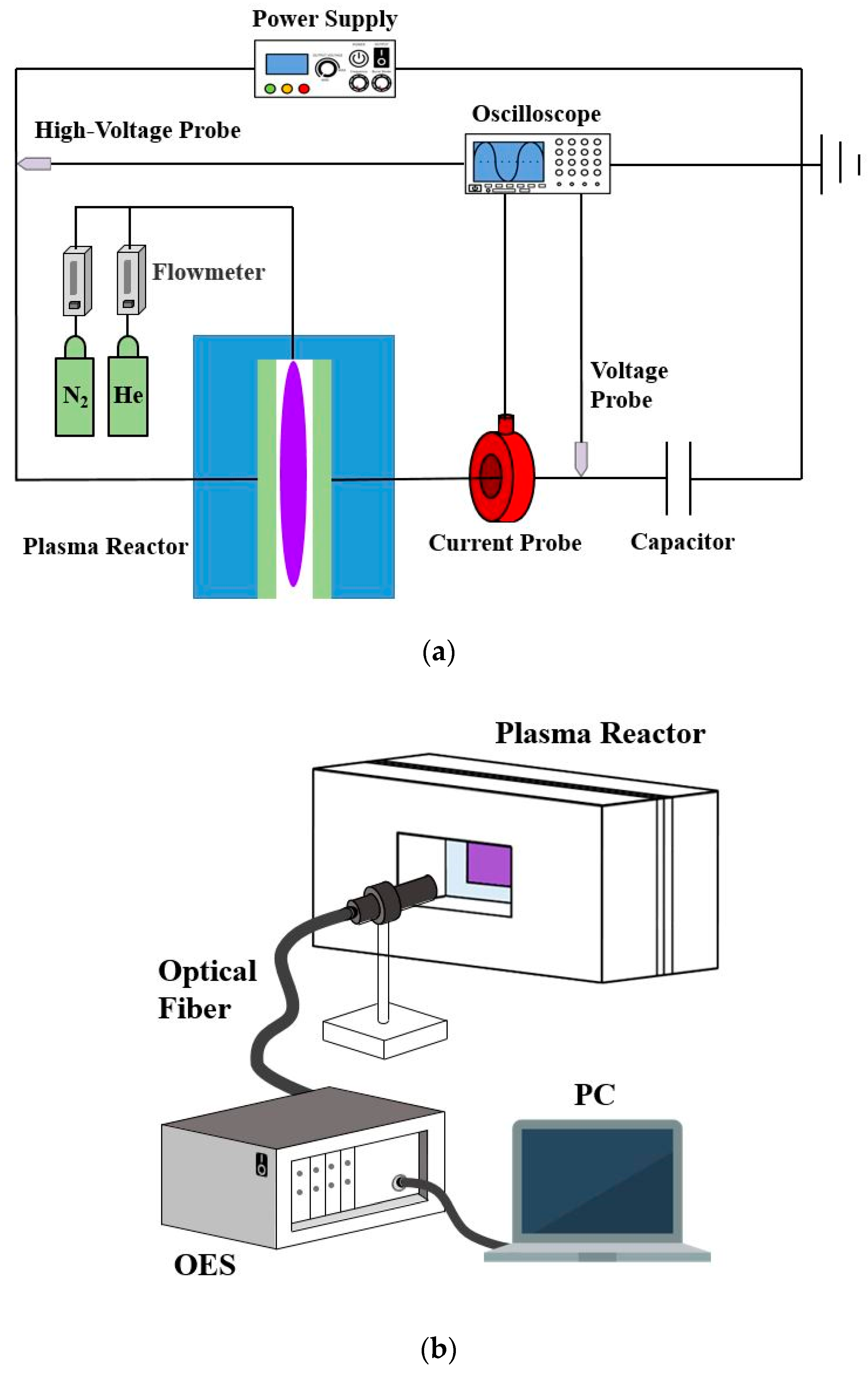
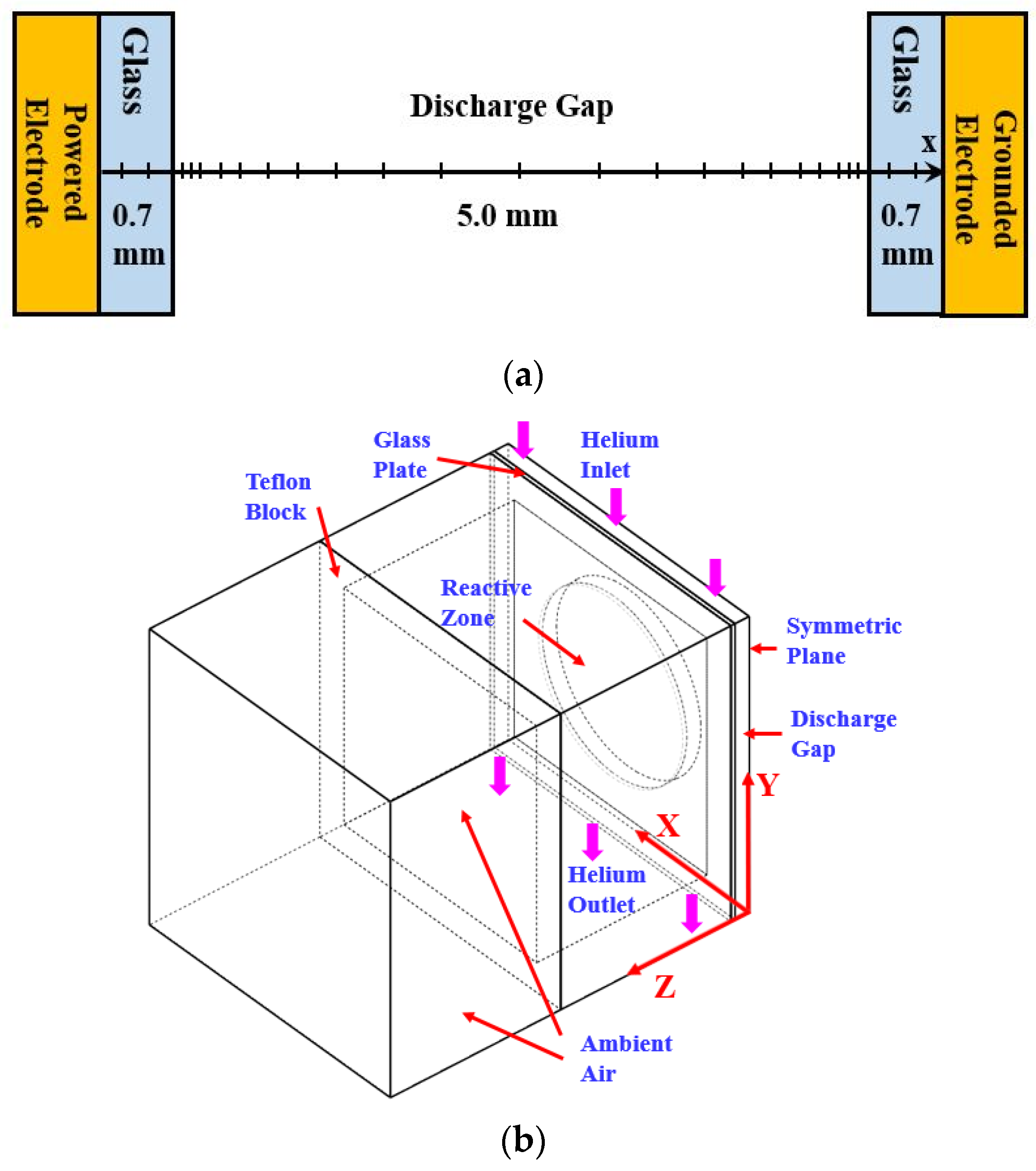
2.1. Experimental Configuration

The experimental configuration used in this work is shown in Figure 1a. A planar reactor is designed with parallel glass plates as transparent electrodes for generating APHeDBDs. One of the surfaces of each glass plate is coated with indium tin oxide as the conductive layer. The reactive area is a circle with a diameter of 30 mm and the discharge gap is fixed at 5 mm. The sinusoidal external power source is supplied with the voltage frequency and amplitude controlled at 16.5 ± 0.1 kHz and 3.5 ± 0.1 kV, respectively. The helium flowrate is controlled at 2 slm and a small amount of N2 admixture (0.1%) is added for measuring the rotational temperature. The discharge voltages and currents are measured by the high-voltage probe (Tektronix P6015A) and current probe (Magnelab CT-C1), respectively, with data stored by the oscilloscope (Keysight Technologies DSOX3054T, 500 MHz and 5.0 GSa s−1). A monitor capacitor with the capacitance of 230 pF is installed at the location after the reactor to measure charge transferred for determining the power consumption by integrating the Lissajous curve [23]. To confirm the discharge uniformity, an ICCD camera (Princeton Instruments PI-MAX4) with an ultraviolet (UV) lens (Nikon PF10545MF-UV) is applied to take photographs from the reactor outlet during the breakdown phase. An OES (AvaSpec ULS2048LUSB2) with the optical fiber located at the lateral side of the reactor as shown in Figure 1b is employed for measuring the average emission spectrum to determine the rotational temperature. The infrared thermal imager (AVIO F50A) is applied to detect the surface temperature of the reactor from the lateral side of the reactor (similar to that shown in Figure 1b) for validating the temperature distribution simulated by the 3D GFM. The gas temperature is measured after the system reaches its thermal equilibrium as the steady-state gas temperature.

2.2. Numerical Method

The 1D PFM and 3D GFM are developed to model the discharge dynamics and steady-state reactor temperature for investigating the thermal behavior of APHeDBDs ignited within the planar reactor. The discharge is simplified as the 1D PFM with its uniformity confirmed by the ICCD photograph taken. The average volumetric heating source calculated by the 1D PFM is adopted as the source term of the energy equation considered in the 3D GFM to model the reactor temperature. The simulation will be performed until the gas temperature used in the 1D PFM is consistent with that obtained by the 3D GFM as described later.

2.2.1. One-Dimensional Plasma Fluid Model (1D PFM)

This section briefs the 1D PFM developed previously [24] with the framework of discharge chemistry including helium and nitrogen related species. Figure 2a shows the numerical domain of the 1D PFM. The discharge gap is 5.0 mm and the thickness of each glass plate is 0.7 mm as used in experimental measurements. The non-uniform mesh is employed with the mesh size covering from 30 μm to 100 μm for capturing discharge dynamics appropriately in the sheath and bulk regions. The mesh independence test has been conducted to ensure the mesh quality.
The continuity equation of each species considered is solved as:
n e , i , u c t + Γ e , i , u c x = S e , i , u c
where n is the species density, Г is the species flux, and the subscripts e, i, and uc represent electron, ion, and neutral species, respectively. The source term S of each continuity equation is evaluated from the discharge chemistry introduced next to account for the generation and destruction reactions of each species. The species flux terms calculated with the drift-diffusion approximation are written as:
Γ e , i = s i g n ( q e , i ) μ e , i n e , i E D e , i n e , i x
Γ u c = D u c n u c x
where q is the species charge, μ is the species mobility, E ( = φ x , φ is the potential) is the electric field, and D is the species diffusivity.
The Poisson equation is solved to calculate the electric field built inside the discharge gap as:
( ε φ ) = c = 1 N c q c n c
where ε ( = ε 0 ε r , ε 0 is the permittivity of free space and ε r is the relative permittivity of each region) is the permittivity of each region and Nc represents the number of charged species.
The electron energy density equation is solved to evaluate the electron temperature for determining rate constants of electron-related reactions and electron transport properties (i.e., De and μ e ) as:
n ε t + Γ ε x = e Γ e E k = 1 N B [ 3 m e M k n e k B ν m , k ( T e T g ) ] n e j = 1 N e ε j k j n j
where n ε ( = 3 2 n e k B T e ) is the electron energy density, k B is the Boltzmann constant, Te is the electron temperature, m e is the electron mass, M is the mass of the background gas (i.e., He or N2), ν m is the frequency of elastic collision, NB is the number of background gases (i.e., NB = 2 for He and N2), Tg is the gas temperature, ε j is the threshold energy of the jth electron-impact reaction, k is the rate constant, and Ne is the number of electron-impact reactions considered in the chemical model. On the right-hand side of Equation (5), the first term is the electron Joule heating evaluating the energy acquired by electrons from the externally applied voltage. The second term calculates the energy loss due to elastic collisions among electrons and neutral background gases (i.e., He and N2). The last term calculates the energy consumption due to electron-impact reactions considered in the discharge chemistry.
It is assumed that charged species accumulate and neutral species quench at the glass surface. The instantaneous voltage of the externally applied power source is assigned on the powered electrode and the potential of the grounded electrode is kept at zero as the boundary conditions for solving the Poisson equation.
The rate constants of electron-impact reactions and electron transport properties are calculated before the simulation by using the Boltzmann equation solver (i.e., Bolsig+ [25]) as look-up tables. The mobilities of ions are adopted from the literature [16,26] with diffusivities evaluated from the Einstein relation. The diffusivities of neutral species are evaluated from the binary diffusion theory [27] with relative parameters that can be found in [28].
The reactions considered in the discharge chemistry are listed in Table 1. The charged species considered include electrons, He+, He2+, N2+, and N4+, to model the conduction currents properly through ionization reactions, association reactions, and recombination reactions. The excited species of helium including Hem and He2* play essential roles for introducing ionization pairs through Penning ionization. The excited species of nitrogen (i.e., N 2 ( A 3   u + ) , N 2 ( B 3 Π g ) , N 2 ( C 3 Π u ) , and N 2 ( a 1 u ) ) are considered to account for the energy released from exothermic reactions. Interactions among helium and nitrogen related species are also included to mimic the realistic discharge chemistry.
The discharge heating source is obtained from the integration of the power released by different heating mechanisms during the cycle as the cyclic average heating source. From the 1D PFM, the cyclic average heating source of the discharge is calculated as:
  S C A P F M = 1 t c y c l e t c y c l e , s t a r t t c y c l e , e n d { k = 1 N B [ 3 m e M k n e k B ν m , k ( T e T g ) ] + i = 1 N i ( q i Γ i E ) + l = r x n R l Δ E l } d t  
where the subscript “CA” represents cyclic average quantity calculated, tcycle is the period of one cycle, Ni is the number of ion species, Rl is the reaction rate of the lth reaction, Δ E is the energy released from the reaction. The first term of the integrand considers the energy released from elastic collisions. The second term of the integrand considers the ion Joule heating under the assumption that energy acquired by ions from the electric field is transferred thoroughly to background gases due to efficient collisions among ions and molecules of background gases. The last term of the integrand considers the energy released from exothermic reactions listed in Table 1.

2.2.2. Three-Dimensional Gas Flow Model (3D GFM)

To simulate the steady-stage gas temperature of the reactor, the commercial software CFD-ACE 2015 was used for building the 3D GFM considering the flow dynamics of the reactor. This section summarizes the governing equations modeled in the 3D GFM while detailed descriptions can be found in [33]. Figure 2b shows the numerical domain including the reactive zone, glass plate, Teflon block, and ambient air environment. Due to the reactor symmetry, the 3D GFM is simplified with the symmetric plane assigned to reduce the model size without losing the accuracy.
The steady-state flow dynamics of the background gases is modeled by solving the mass and momentum conservation equations as:
( ρ V ) = 0
( ρ V V ) = p + τ + S M
where ρ is the density of the background gas (i.e., air or He), V is the velocity vector, p represents the pressure of the background gas, τ is the viscous stress tensor, and S M is the momentum source term to calculate the buoyance force resulting in the cooling of natural convection on the reactor surface.
The steady-state gas temperature of the reactor is modeled by solving the energy equation (total enthalpy) as:
( ρ V h T ) = ( λ T ) + ( V τ ) + S G F M
where h T ( = h + 1 2 × x = 1 3 u x 2 , h is the enthalpy and u represents the velocity component) is the total enthalpy, λ is the thermal conductivity of the background gas, and S G F M is the average volumetric heating source obtained from the 1D PFM. The S G F M is applied to the reactive zone as the average volumetric heating source evaluated as:
S G F M = S S C A P F M = m = 1 N c e l l ( S C A P F M , m × w m ) d g a p
where the subscript “SCA” represents the spatial cyclic average quantity calculated, Ncell is the cell number used in the 1D PFM for the discharge gap, w is the cell width, d g a p is the discharge gap as 5 mm, and the subscript m represents the mth cell.
In the discharge gap, the helium flow is provided as the inlet boundary condition from the top of the reactor. We test whether the small amount of N2 addition had only a minor effect on the simulated gas temperature; therefore, the small amount of N2 addition is neglected in the 3D GFM. The outlet boundary condition is assigned on boundaries of ambient air around the reactor to allow air flows in and out of the boundaries as the natural convection is built. The solid boundaries are assigned as zero-gradient condition as:
n ( k T ) = 0
The thermal conductivities of the Teflon block and glass plate are 0.25 W m−1 K−1 and 1.1 W m−1 K−1, respectively. The temperature-dependent thermal properties of helium and air are evaluated by the kinetic theories which can be found in [33]. This is tested and it is concluded that the simulated temperature distribution is insensitive to the size of the Teflon block. The mesh independence test has been conducted for the 3D GFM to ensure the mesh quality.

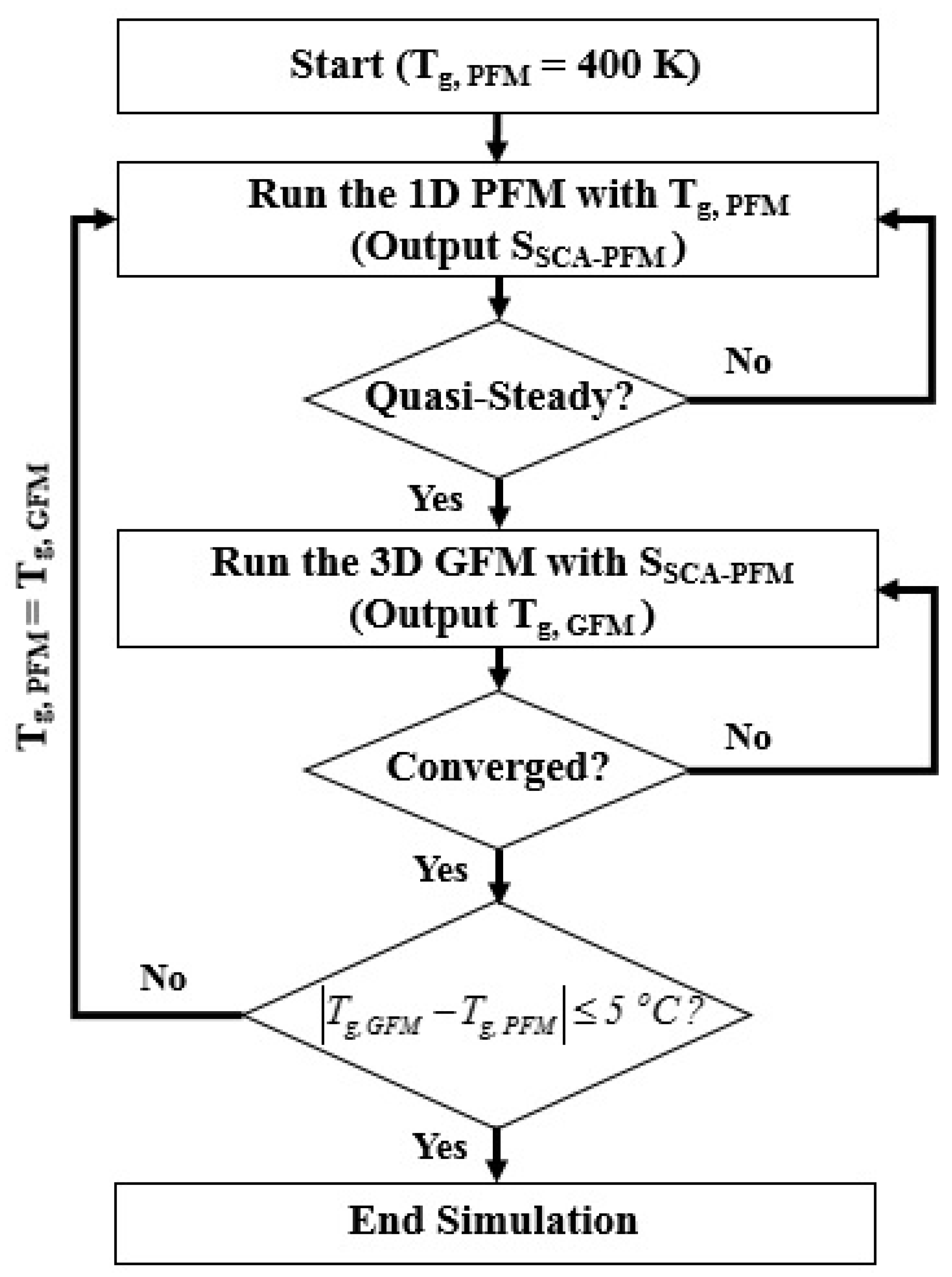
2.2.3. Model Coupling

The 1D PFM and 3D GFM are developed to model the discharge dynamics and gas temperature of the reactor separately and combined with the weak coupling as shown in Figure 3 since it is efficient to obtain the individual solution separately for two models with different characteristic times [34]. The simulation is performed from the 1D PFM by adopting the initial gas temperature Tg,PFM as 400 K until the quasi-steady solution is obtained. The cyclic average power consumption and average volumetric heating source are monitored as the criteria of the quasi-steady solution and are written as:
P C A P F M k P C A P F M k 1 P C A P F M k 0.01
S S C A P F M k S S C A P F M k 1 S S C A P F M k 0.01
where the superscripts k and k − 1 are the quantities obtained in the current and previous time steps, respectively. The cyclic average power consumption of the simulated discharge P C A P F M is evaluated by integrating from the voltage and total current at each time step obtained in the 1D PFM over the whole cycle as:
P C A P F M = 1 t c y c l e t c y c l e , s t a r t t c y c l e , e n d V I d t o t a l   t
where I t o t a l is the total current including the conduction currents of charged species and the displacement current. Then quasi-steady solution of the 1D PFM is used to calculate the average volumetric heating source which is adopted as the source term of the energy equation considered in the 3D GFM for modeling the temperature of the reactor. After obtaining the steady-state solution of the 3D GFM, the average gas temperature in the reactive zone is calculated as Tg,GFM. If the gas temperature obtained from the 3D GFM is not consistent with the gas temperature Tg,PFM used in the 1D PFM, the Tg,PFM is replaced with the Tg,GFM for running the 1D PFM again. The converged solution will be obtained until the Tg,PFM used is consistent with the Tg,GFM calculated with the following criterion:
| T g , P F M T g , G F M | 5   C   o
Generally, two or three iterations are required to obtain the converged solution. The converged solution is analyzed and presented in Section 3.

3. Results and Discussion

The first part of this section validates the method developed. The discharge uniformity is confirmed with the ICCD photograph to justify the simplification of 1D PFM. The simulated discharge characteristics including the current density and power consumption are compared with experimental measurements. The simulated average gas temperature of the reactive zone is compared with the rotational temperature determined, and the surface temperature of the reactor is compared with that detected by the IR thermal imager. The second part of this section analyzes the dominant heating mechanisms of APHeDBDs. The contribution of each heating mechanism is presented.

3.1. Model Validation

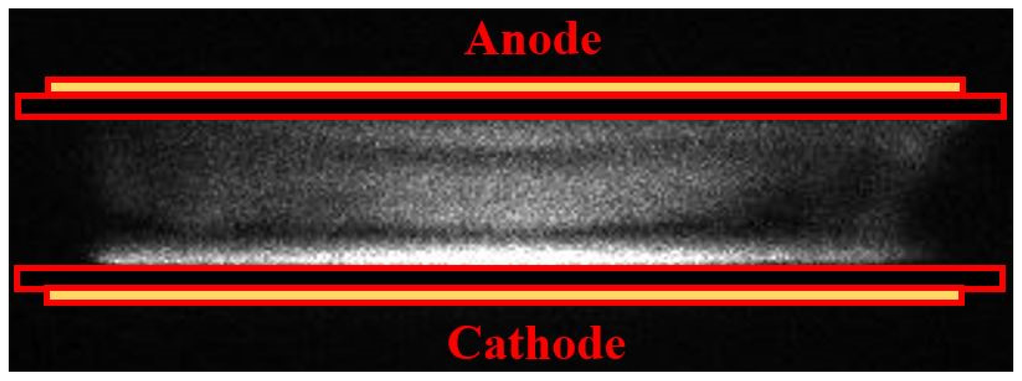
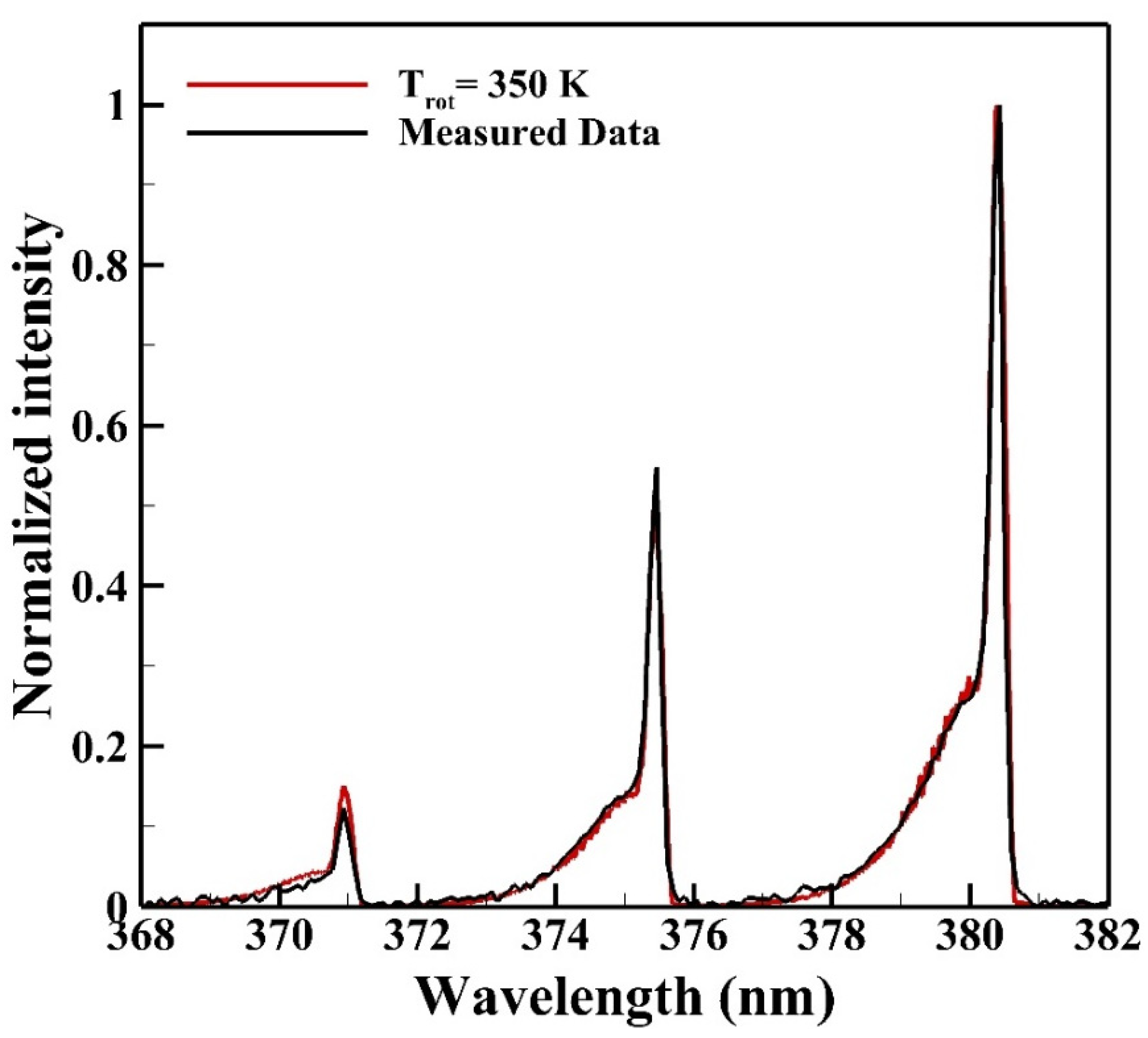
3.1.1. Discharge Uniformity

In this work, the APHeDBD is simplified with the 1D PFM under the assumption of uniform discharge. However, it is noted that APHeDBDs may not be uniform under various operating conditions [17,18]. The discharge uniformity under current operating conditions is confirmed by the ICCD photograph taken during the breakdown of a typical cycle with the 1 μs exposure time as shown in Figure 4. The uniform discharge irradiation occurs near the surface of the glass plate covering the grounded electrode due to excited species generated by energetic electrons in the cathode fall region. Uniform discharges generated in the planar reactors under similar operating conditions were reported by other groups with similar discharge structure presented [16,17], supporting the uniform discharges observed in this work. The confirmed discharge uniformity justifies the application of the 1D PFM for modeling the APHeDBDs.

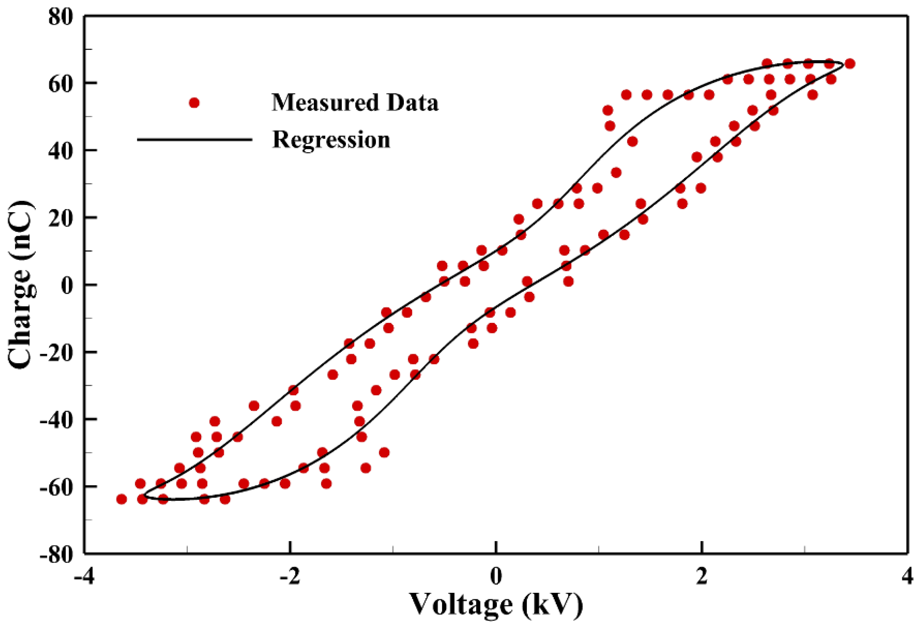
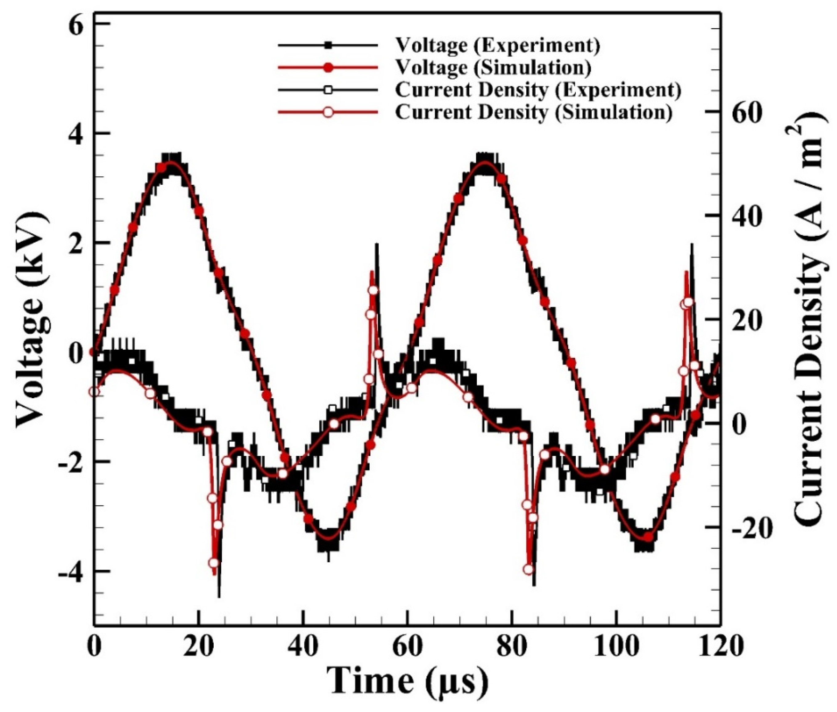
3.1.2. Power Consumption

The power consumption measured is obtained by integrating the Lissajous curve measured in a typical cycle from the capacitor as shown in Figure 5. It is noted that only a few data points are plotted for presentation purposes and the solid line is regressed from measured data to calculate the power consumption. The average power consumption measured from measurements is around 2.1 W.
Figure 6 shows the comparison between the measured and simulated current densities of a typical cycle. It is noted that the experimental current densities in the positive half period (HP) are similar to those in the negative HP, which shows that the discharge is symmetrical under current operating conditions. The simulated current density reaches around 29 A m−2 which agrees with that measured on average as 35 A m−2. The simulated cyclic average power consumption can be calculated from the integration of the externally applied voltage and simulated current as 2.0 W which agrees with the measured average power consumption as 2.1 W.

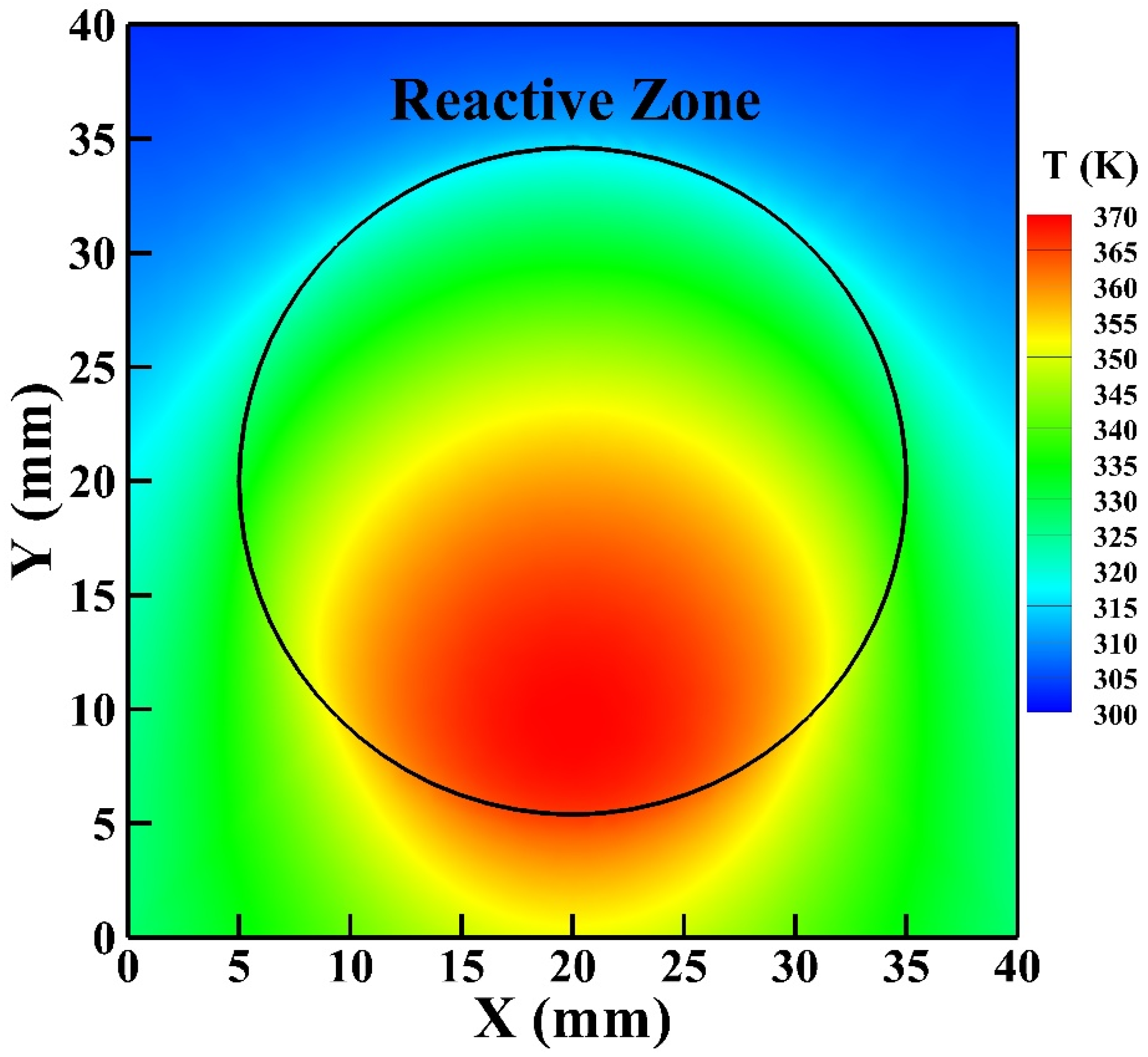
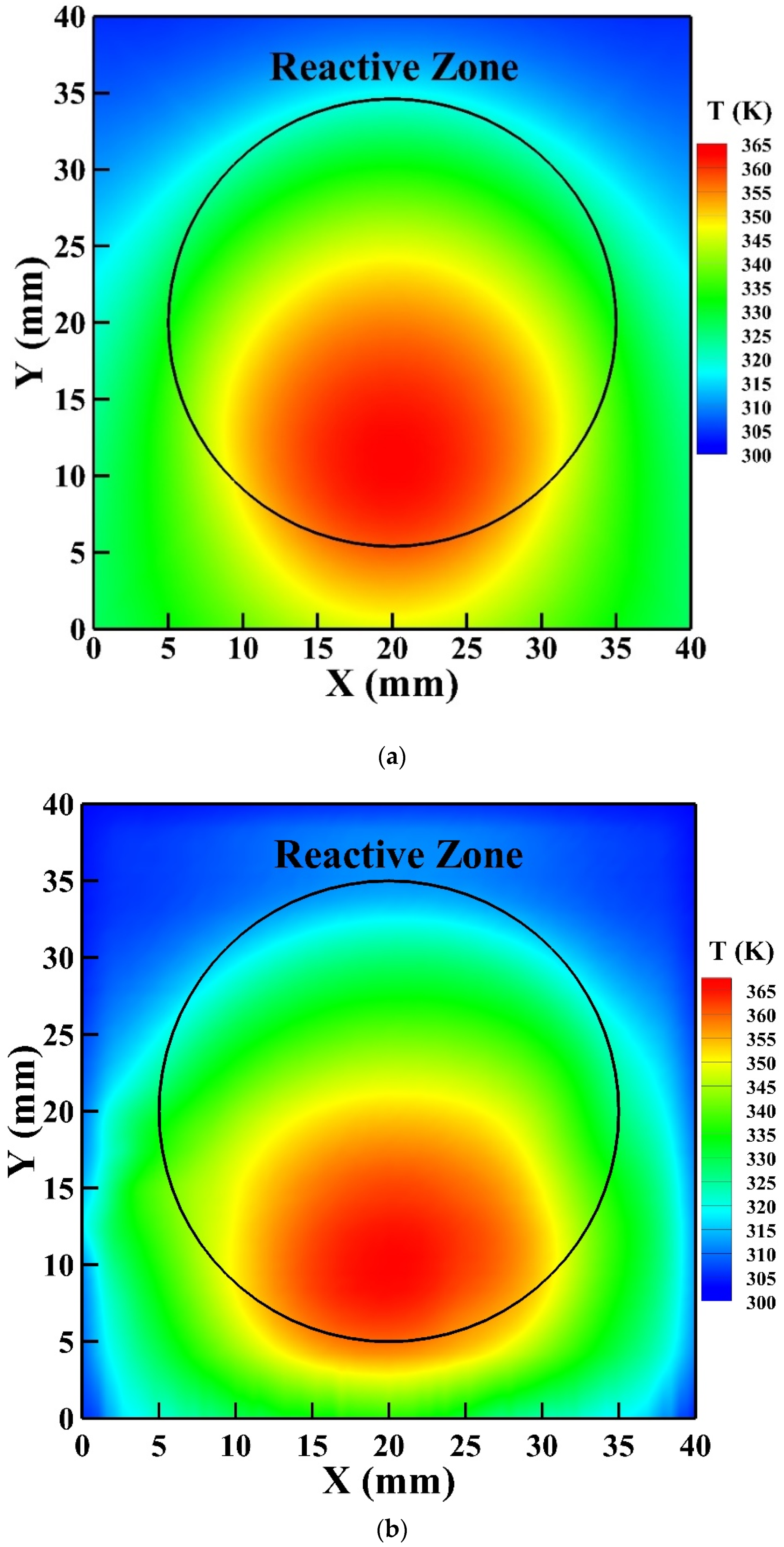
3.1.3. Reactor Temperature

Figure 7 shows the average emission spectrum of N2 SPS measured from the reactive zone for determining the rotational temperature. The red solid line labeled as “Trot” is the theoretical spectrum calculated from the commercial software Specair with theories of quantum mechanics for comparing with the average measured emission spectrum to determine the rotational temperature. The rotational temperature determined is 350 K.
The simulated heating power calculated by the 1D PFM in the reactive zone is around 1.8 W. In other words, around 90% of the average power consumption contributes to gas heating under current operating conditions, which is similar to the simulated result obtained for a helium microplasma operated under atmospheric pressure [9]. The volumetric heating source calculated by Equation (10) is adopted as the source term of the energy equation considered in the 3D GFM for modeling the temperature distribution of the reactor.
Figure 8 shows the gas temperature in the symmetric plane of the reactor. The helium gas flows from the inlet on the reactor top and exits from the outlet on the reactor bottom. The helium flow is supplied at room temperature (300 K) and is heated as the flow passes the reactive zone. It is observed that the high-temperature zone moves slightly downward from the central region of the reactive zone because of the convective effect with the highest gas temperature reaching around 373 K. The average simulated gas temperature of the reactive zone is around 346 K which is close to the rotational temperature determined.
To further validate the 3D GFM developed, the simulated surface temperature of the reactor is compared with that detected by the IR thermal imager as presented in Figure 9a,b, respectively. Similarly, the high-temperature zone of the simulated surface temperature moves downward from the central region of the reactive zone as explained previously, which agrees with the temperature distribution detected by the IR thermal imager. The simulated highest surface temperature is 362 K, which is in good agreement with that detected by the IR thermal imager as 365 K with an uncertainty of 2 K.
Generally, the simulated results capture the thermal behavior of the APHeDBDs.

3.2. Analysis of Atmospheric-Pressure Helium Dielectric-Barrier Discharges (APHeDBDs) Gas Heating

To understand the gas heating behavior of APHeDBDs, the simulated cyclic average power consumption is analyzed and the contributions of different heating mechanisms are presented.

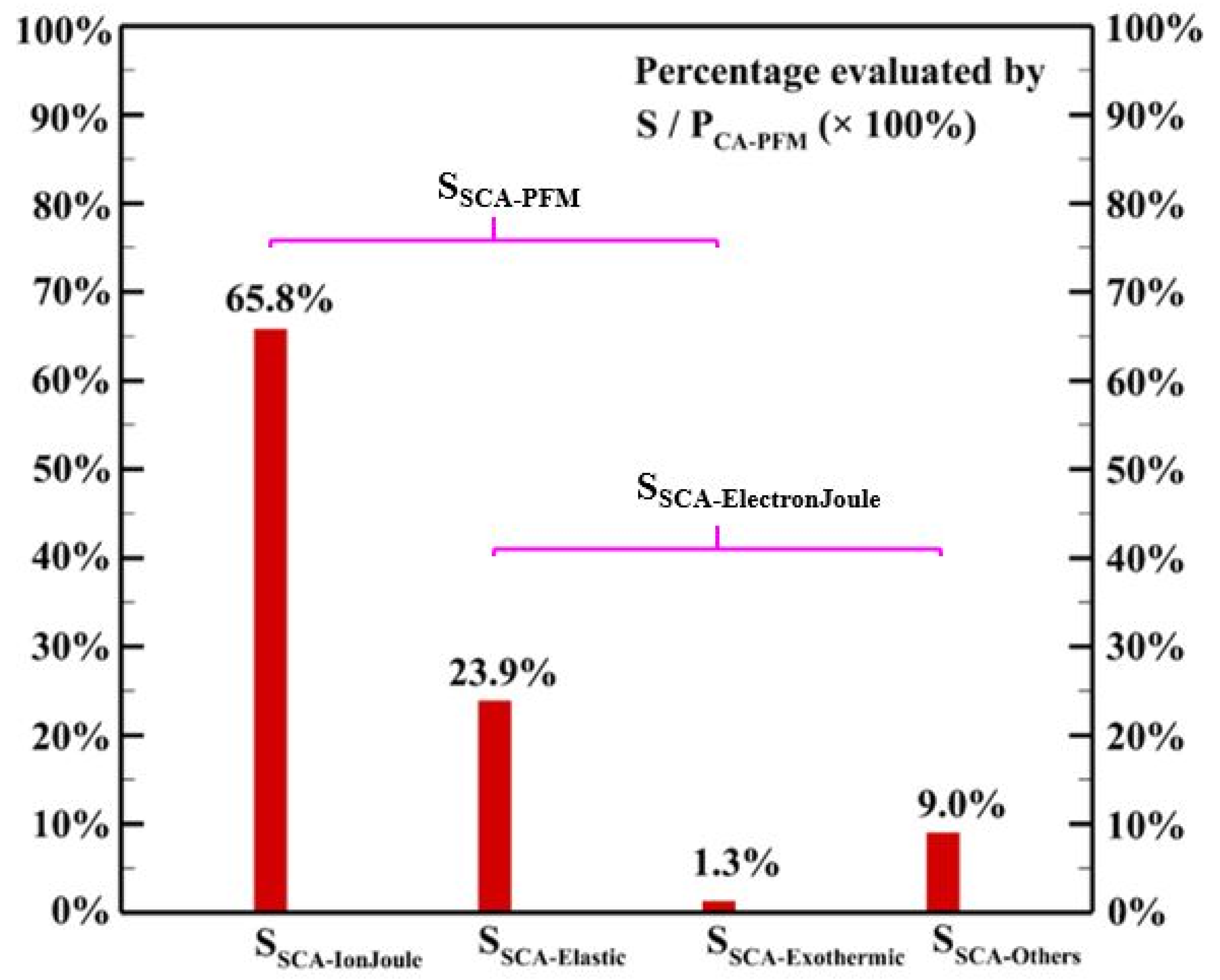
3.2.1. Analysis of Power Consumption

Figure 10 shows the details of the simulated spatial cyclic average power consumption of different mechanisms considered in the 1D PFM. The cyclic average power consumption of the discharge is equal to the power acquired by charged species as:
P C A P F M = S S C A E l e c t r o n J o u l e + S S C A I o n J o u l e
where S S C A E l e c t r o n J o u l e is the spatial cyclic average electron Joule heating and S S C A I o n J o u l e is the spatial cyclic average ion Joule heating. Moreover, the S S C A E l e c t r o n J o u l e can be further categorized as:
S S C A E l e c t r o n J o u l e = S S C A E l a s t i c + S S C A E x o t h e r m i c + S S C A O t h e r s
where S S C A E l a s t i c is the heating source due to elastic collisions among electrons and background gases, S S C A E x o t h e r m i c is the heating power released from exothermic reactions considered in the discharge chemistry, and S S C A O t h e r s is the power consumed for generating other reactive species in the discharge. Figure 10 shows that around 90% of the cyclic average power consumption P C A P F M goes to gas heating through elastic collision, ion Joule heating, and exothermic reactions considered. It is observed that elastic collision and ion Joule heating are the dominant heating mechanisms contributing 23.9% and 65.8% of the power consumption, respectively, to the heating source, which is different from the simulated results obtained in [21,22] for helium discharges excited by the radio-frequency power sources showing that elastic collision is the dominant heating source. Although a few exothermic reactions release a large amount of energy in each reaction, the exothermic reactions considered contribute only a minor amount of energy to the heating source due to the low reaction rates.

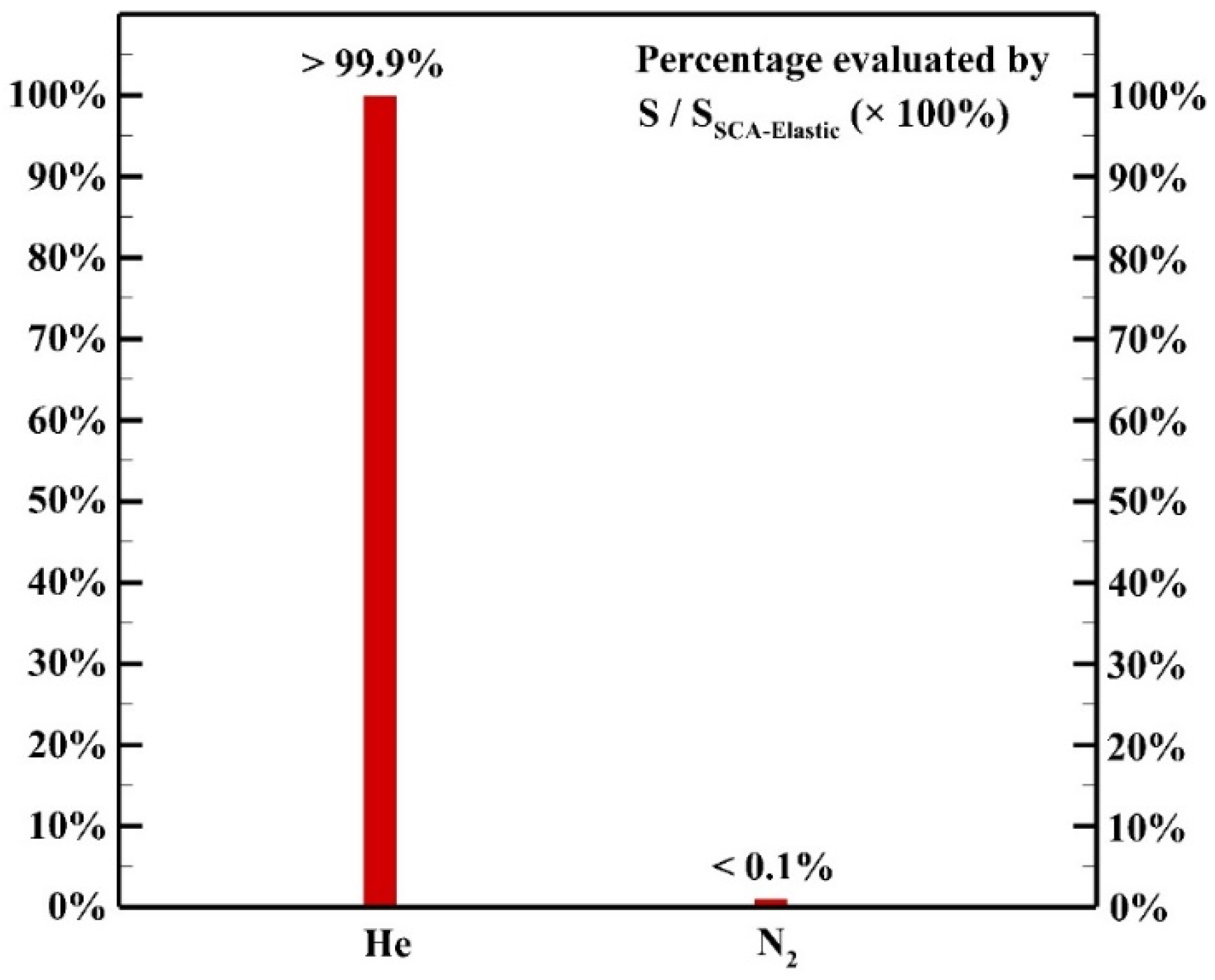
3.2.2. Elastic Collision

Figure 11 shows the contributions of elastic collisions among electrons and different background neutral gases. Although the energy exchange of each elastic collision process between an electron and a background molecule is inefficient due to large mass difference, the high collision frequency results in a remarkable contribution to the heating source as reported by other groups [9,21,22] in atmospheric pressure helium discharges. The collisions of electrons and helium atoms contribute to more than 99.9% of the heating source of elastic collision while the collisions of electrons and N2 molecules contribute to less than 0.1% of the heating source of elastic collision since the concentration of helium atoms is much higher than that of the N2 molecules.

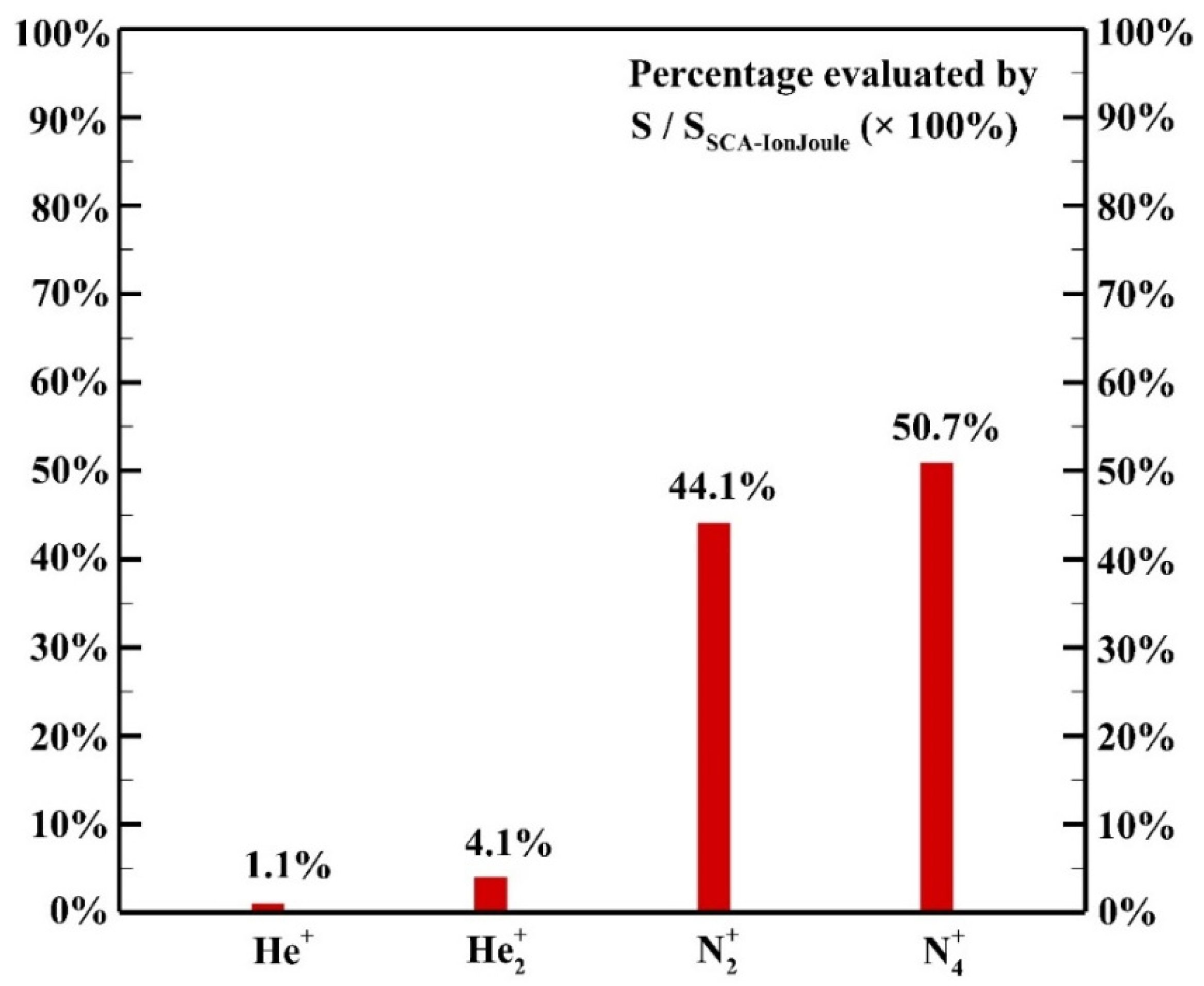
3.2.3. Ion Joule Heating

The contribution of each species to the ion Joule heating is shown in Figure 12. It is assumed that the power acquired by the ion species is transferred to background gases thoroughly due to the efficient collisions among ion species and background gases with comparable masses. Among ion species, the species N2+ and N4+ contribute 44.1% and 50.7%, respectively, to the heating source of ion Joule heating as the dominant species though the concentration of N2 is much lower than that of helium.
To further study the contribution of each ion species, Figure 13 shows the spatial average density changes of ion species during the breakdown in a typical positive HP. For the presentation purpose, the horizontal axis is rescaled. As the breakdown occurs, the number densities of He+ and He2+ increase simultaneously due to:
e + H e 2 e + H e +             ( R 4 )
2 H e + H e + H e + H e 2 +       ( R 17 )
It is observed that the number density of N2+ increases faster than those of He+ and He2+ because of the high rate constant of Penning ionization:
H e m + N 2 e + H e + N 2 +         ( R 40 )
As the density of N2+ increases, the density of N4+ increases due to the fast associative process:
    N 2 + + N 2 + H e N 4 + + H e         ( R 31 )
As a result, the species N4+ is the dominant ion species. Similar simulated results can be found in [13,15,16] showing that N4+ is the dominant ion species if the concentration of N2 admixture is higher than a certain level (e.g., ~tens of ppm) in APHeDBDs. Therefore, the species N4+ has the highest contribution to the ion Joule heating.

3.2.4. Spatial Distributions of Heating Sources

Before investigating the spatial distributions of heating sources, it is essential to understand the cyclic average spatial distributions of species densities of electrons and dominant ions as shown in Figure 14 with the distribution of electron temperature included. It is noted that the sheath regions are built near the glass surfaces (i.e., at 0.7 mm and 5.7 mm) since the intensive electric fields (not shown) are built due to the distribution of charged species. The intensive electric field that is built results in energetic electrons with high electron temperature, which leads to high reaction rates in the sheath region. Similar simulated results with sheath regions were observed for atmospheric pressure helium dielectric barrier discharges excited by kHz power sources [16,35]. It is observed that the electron temperature reaches around 3.9 eV as the maximum in the sheath region, while the density of N4+ reaches around 5.2 × 10¹⁶ m−3. Both the species densities of electron and N4+ reach the level of 1016 m−3 in the central bulk region.
Figure 15 shows the cyclic average heating sources of different heating mechanisms. The simulated average total heating source is around 5.6 × 10⁵ W m−3 with the maximum reaching 3.5 × 10⁶ W m−3 in the sheath region due to the contribution of ion Joule heating. The total heating source reaches the level of 105 W m−3 in the bulk region due to the contribution of elastic collision. It is observed that the heating source of elastic collision increases to the maximum near the sheath region since the local electron density and electron temperature are higher than those in the central region. Similarly, the heating sources of ion Joule heating and exothermic reactions reach the maxima because of the high species densities generated and the electric field built in the sheath region.

4. Conclusions

The present work studies the thermal behavior of APHeDBDs with a small amount of N2 addition for temperature measurements by numerical simulations and experimental measurements. The dynamics of APHeDBDs generated in a planar reactor is modeled by the 1D PFM with the discharge chemistry including He and N2 related species to calculate the spatial cyclic average heating source considering elastic collision, ion Joule heating, and exothermic reactions. The average heating source obtained by the 1D PFM is adopted as the source term of the energy equation considered in the 3D GFM for modeling the temperature of the reactor. The 1D PFM and 3D GFM are coupled weakly to obtain the converged solution until the gas temperature used in the 1D PFM is consistent with that obtained in the 3D GFM.
The discharge uniformity is verified by the ICCD photograph to justify the application of the 1D PFM for modeling the uniform discharge. The simulated current density reaches 29 A m−2 which is close to that measured as 35 A m−2. The simulated power consumption is around 2.0 W which is in good agreement with the average measured power consumption of 2.1 W. The simulated average gas temperature in the reactive zone is about 346 K which is also close to the rotational temperature determined from the emission spectrum of N2 SPS. The high-temperature zone of the simulated surface temperature of the reactor moves slightly downward due to the convective effect, which is similar to the temperature distribution detected by the IR thermal imager. Moreover, the maximum simulated surface temperature is 362 K which is close to that measured as 365 K. In general, the numerical simulations capture the thermal behavior of the APHeDBDs.
The analysis shows that elastic collision and ion Joule heating are dominant heating mechanisms contributing 23.9% and 65.8% to the heating source, respectively. Detailed analysis shows that elastic collisions of electrons and helium atoms contribute more than 99.9% of the heating source of elastic collision since the concentration of He atoms is much higher than that of N2 molecules. Among ion species, N2+ and N4+ are dominant species contribute 44.1% and 50.7% to the heating source of ion Joule heating, respectively. The simulated result shows that the Penning ionization of excited He species and N2 molecules leads to the abundant generation of N2+ while the fast associative process results in the dominant ion N4+. The simulated average total heating source is around 5.6 × 10⁵ W m−3 with the maximum reaching 3.5 × 10⁶ W m−3 in the sheath region due to the contribution of ion Joule heating.

Author Contributions

Conceptualization, K.-M.L.; Data curation, K.-C.W.; Formal analysis, K.-C.W.; Funding acquisition, K.-M.L.; Methodology, K.-M.L.; Resources, K.-C.W.; Supervision, K.-M.L.; Validation, Y.-S.C. and S.-Y.C.; Visualization, Y.-S.C. and S.-Y.C.; Writing—original draft, K.-M.L. All authors have read and agreed to the published version of the manuscript.

Funding

This research was funded by the Ministry of Science and Technology (MOST) in Taiwan through Grant No. 109-2221-E-194-017-MY2.

Acknowledgments

This research was also financially supported by the Center for Innovative Research on Aging Society (CIRAS) and the Advanced Institute of Manufacturing with High-tech Innovations (AIM-HI) from The Featured Areas Research Center Program within the framework of the Higher Education Sprout Project by the Ministry of Education (MOE) in Taiwan. Finally, the authors also thank Ying-Hao Liao and Chong-Sin Wu for the support of measurements conducted at National Chiao Tung University.

Conflicts of Interest

The authors declare no conflict of interest.

References

  1. Nastuta, V.; Popa, G. Surface oxidation and enhanced hydrophilization of polyamide fiber surface after He/Ar atmospheric pressure plasma exposure. Rom. Rep. Phys. 2019, 71, 413. [Google Scholar]
  2. Cools, P.; Asadian, M.; Nicolaus, W.; Declercq, H.; Morent, R.; de Geyter, N. Surface treatment of PEOT/PBT (55/45) with a dielectric barrier discharge in Air, Helium, Argon and Nitrogen at medium pressure. Materials 2018, 11, 391. [Google Scholar] [CrossRef] [PubMed] [Green Version]
  3. Nagatsu, M.; Sugiyama, K.; Motrescu, I.; Ciolan, M.A.; Ogino, A.; Kawamura, N. Surface modification of fluorine contained resins using an elongated parallel plate electrode type dielectric barrier discharge device. J. Photopolym. Sci. Technol. 2018, 31, 379–383. [Google Scholar] [CrossRef]
  4. von Woedtke, T.H.; Reuter, S.; Masur, K.; Weltmann, K.D. Plasmas for medicine. Phys. Rep. Rev. Sec. Phys. Lett. 2013, 530, 291–320. [Google Scholar] [CrossRef]
  5. Setsuhara, Y. Low-temperature atmospheric-pressure plasma sources for plasma medicine. Arch. Biochem. Biophys. 2016, 605, 3–10. [Google Scholar] [CrossRef]
  6. Li, H.P.; Zhang, X.F.; Zhu, X.M.; Zheng, M.; Liu, S.F.; Qi, X.; Wang, K.P.; Chen, J.; Xi, X.Q.; Tan, J.G.; et al. Translational plasma stomatology: Applications of cold atmospheric plasmas in dentistry and their extension. High Volt. 2017, 2, 188–199. [Google Scholar] [CrossRef]
  7. Majstorovic, G.L.; Jovovic, J.; Sisovic, N.M. The analysis of nitrogen rotational and vibrational bands in a helium microhollow gas discharge. Contrib. Plasma Phys. 2017, 57, 282–292. [Google Scholar] [CrossRef]
  8. Bruggeman, P.J.; Sadeghi, N.; Schram, D.C.; Lins, V. Gas temperature determination from rotational lines in non-equilibrium plasmas: A review. Plasma Sources Sci. Technol. 2014, 23, 023001. [Google Scholar] [CrossRef] [Green Version]
  9. Wang, Q.; Doll, F.; Donnelly, V.M.; Economou, D.J.; Sadeghi, N.; Franz, G.F. Experimental and theoretical study of the effect of gas flow on gas temperature in an atmospheric pressure microplasma. J. Phys. D Appl. Phys. 2007, 40, 4202–4211. [Google Scholar] [CrossRef]
  10. Nersisyan, G.; Graham, W.G. Characterization of a dielectric barrier discharge operating in an open reactor with flowing helium. Plasma Sources Sci. Technol. 2004, 13, 582–587. [Google Scholar] [CrossRef]
  11. Bibinov, N.K.; Fateev, A.A.; Wiesemann, K. On the influence of metastable reactions on rotational temperatures in dielectric barrier discharges in He-N2 mixtures. J. Phys. D-Appl. Phys. 2001, 34, 1819–1826. [Google Scholar]
  12. Lazarou, C.; Belmonte, T.; Chiper, A.S.; Georghiou, G.E. Numerical modelling of the effect of dry air traces in a helium parallel plate dielectric barrier discharge. Plasma Sources Sci. Technol. 2016, 25, 055023. [Google Scholar]
  13. Lazarou, C.; Koukounis, D.; Chiper, A.S.; Costin, C.; Topala, I.; Georghiou, G.E. Numerical modeling of the effect of the level of nitrogen impurities in a helium parallel plate dielectric barrier discharge. Plasma Sources Sci. Technol. 2015, 24, 035012. [Google Scholar]
  14. Martens, T.; Bogaerts, A.; Brok, W.J.M.; von Dijk, J. The influence of impurities on the performance of the dielectric barrier discharge. Appl. Phys. Lett. 2010, 96, 091501. [Google Scholar]
  15. Martens, T.; Bogaerts, A.; Brok, W.J.M.; Dijk, J.V. The dominant role of impurities in the composition of high pressure noble gas plasmas. Appl. Phys. Lett. 2008, 92, 041504. [Google Scholar]
  16. Mangolini, L.; Anderson, C.; Heberlein, J.; Kortshagen, U. Effects of current limitation through the dielectric in atmospheric pressure glows in Helium. J. Phys. D Appl. Phys. 2004, 37, 1021–1030. [Google Scholar]
  17. Massines, F.; Rabehi, A.; Decomps, P.; Gadri, R.B.; Segur, P.; Mayoux, C. Experimental and theoretical study of a glow discharge at atmospheric pressure controlled by dielectric barrier. J. Appl. Phys. 1998, 83, 2950–2957. [Google Scholar]
  18. Radu, I.; Bartnikas, R.; Czeremuszkin, G.; Wertheimer, M.R. Diagnostics of dielectric barrier discharges in noble gases: Atmospheric pressure glow and pseudoglow discharges and spatio-temporal patterns. IEEE Trans. Plasma Sci. 2003, 31, 411–421. [Google Scholar]
  19. Jugroot, M. Neutral gas heating in helium microplasmas. J. Appl. Phys. 2009, 105, 023304. [Google Scholar]
  20. Kang, W.S.; Kim, H.S.; Hong, S.H. Gas temperature effect on discharge-mode characteristics of atmospheric-pressure dielectric barrier discharge in a helium-oxygen mixture. IEEE Trans. Plasma Sci. 2010, 38, 1982–1990. [Google Scholar]
  21. Wang, Q.; Yu, X.L.; Wang, D.Z. Numerical study on the gas heating mechanism in pulse-modulated radio-frequency glow discharge. Chin. Phys. B 2017, 26, 035201. [Google Scholar] [CrossRef]
  22. Zhang, X.F.; Wang, Z.B.; Nie, Q.Y.; Li, H.P.; Bao, C.Y. Influences of gas flowing on the features of a Helium radio-frequency atmospheric-pressure glow discharge. Appl. Therm. Eng. 2014, 72, 82–89. [Google Scholar] [CrossRef] [Green Version]
  23. Ashpis, E.; Laun, M.C.; Griebeler, E.L. Progress toward Accurate Measurements of Power Consumptions of DBD Plasma Actuators. AIAA Report No.20120823. In Proceedings of the 50th AIAA Aerospace Sciences Meeting Including the New Horizons Forum and Aerospace Exposition, Nashville, Tennessee, 9–12 January 2012. [Google Scholar]
  24. Lin, K.M.; Hung, C.T.; Hwang, F.N.; Smith, M.R.; Yang, Y.W.; Wu, J.S. Development of a parallel semi-implicit two-dimensional plasma fluid modeling code using finite-volume method. Comput. Phys. Commun. 2012, 183, 1225–1236. [Google Scholar] [CrossRef]
  25. Hagelaar, G.J.M.; Pitchford, L.C. Solving the Boltzmann equation to obtain electron transport coefficients and rate coefficients for fluid models. Plasma Sources Sci. Technol. 2005, 14, 722–733. [Google Scholar] [CrossRef]
  26. Yuan, X.; Raja, L.L. Computational study of capacitively coupled high-pressure glow discharges in helium. IEEE Trans. Plasma Sci. 2003, 31, 495–503. [Google Scholar] [CrossRef]
  27. Bird, R.B.; Stewart, W.E.; Lightfoot, E.N. Transport Phenomena; John Wiley & Sons: New York, NY, USA, 2007. [Google Scholar]
  28. Poling, B.E.; Prausnitz, J.M.; O’Connell, J.P. The Properties of Gases and Liquids; McGraw-Hill: New York, NY, USA, 2001. [Google Scholar]
  29. Martens, T.; Bogaerts, A.; Brok, W.; van Dijk, J. Computer simulations of a dielectric barrier discharge used for analytical spectrometry. Anal. Bioanal. Chem. 2007, 388, 1583–1594. [Google Scholar] [CrossRef]
  30. Breden, D.; Raja, L.L. Computational study of the interaction of cold atmospheric Helium plasma jets with surfaces. Plasma Sources Sci. Technol. 2014, 23, 065020. [Google Scholar] [CrossRef] [Green Version]
  31. Tochikubo, F.; Uchida, S.; Yasui, H.; Sato, K. Numerical simulation of NO oxidation in dielectric barrier discharge with microdischarge formation. Jpn. J. Appl. Phys. 2009, 48, 076507. [Google Scholar] [CrossRef]
  32. Kossyi, I.A.; Kostinsky, A.Y.; Matveyev, A.A.; Silakov, V.P. Kinetic scheme of the non-equilibrium discharge in nitrogen-oxygen mixtures. Plasma Sources Sci. Technol. 1992, 1, 207–220. [Google Scholar] [CrossRef]
  33. CFD-ACE+ User’s Manual 2015; ESI Group: Paris, France, 2015.
  34. Lin, K.M.; Hu, M.H.; Hung, C.T.; Wu, J.S.; Hwang, F.N.; Chen, Y.S.; Cheng, G. A parallel hybrid numerical algorithm for simulating gas flow and gas discharge of an atmospheric-pressure plasma jet. Comput. Phys. Commun. 2012, 183, 2550–2560. [Google Scholar] [CrossRef]
  35. Wang, D.; Wang, Y.; Liu, C. Multipeak behavior and mode transition of a homogeneous barrier discharge in atmospheric pressure helium. Thin Solid Films 2006, 506, 384. [Google Scholar] [CrossRef]
Figure 1. The schematic diagrams of (a) the experimental configuration; (b) the measurement of the emission spectrum with an optical emission spectrometer (OES).
Applsci 10 07583 g001
Figure 2. The numerical domains: (a) 1D PFM; (b) three-dimensional gas flow model (3D GFM).
Applsci 10 07583 g002
Figure 3. The flowchart of the model coupling.
Applsci 10 07583 g003
Figure 4. The intensified CCD (ICCD) photograph is taken with the 1 μs exposure time during the breakdown to confirm the discharge uniformity.
Applsci 10 07583 g004
Figure 5. The Lissajous curve of a typical discharge cycle to evaluate the measured power consumption.
Applsci 10 07583 g005
Figure 6. The simulated and measured current densities of atmospheric-pressure helium dielectric-barrier discharges (APHeDBDs) generated in the planar reactor.
Applsci 10 07583 g006
Figure 7. The rotational temperature of the reactive zone is determined as 350 K from the emission spectrum of the N2 second positive system (SPS).
Applsci 10 07583 g007
Figure 8. The gas temperature distribution in the symmetric plane of the reactor.
Applsci 10 07583 g008
Figure 9. The surface temperature of the reactor: (a) simulated by the 3D GFM; (b) measured by the infrared (IR) thermal imager.
Applsci 10 07583 g009
Figure 10. The simulated spatial cyclic average power consumption of different mechanisms.
Applsci 10 07583 g010
Figure 11. The contribution of each background gas to the heating source of elastic collision.
Applsci 10 07583 g011
Figure 12. The contribution of each species to the ion Joule heating.
Applsci 10 07583 g012
Figure 13. The spatial average densities of ion species during the breakdown in the positive half period (HP).
Applsci 10 07583 g013
Figure 14. The cyclic average distributions of electron, dominant ion N4+, and electron temperature (Te) in the gap.
Applsci 10 07583 g014
Figure 15. The cyclic average distributions of heating sources of different heating mechanisms in the gap.
Applsci 10 07583 g015
Table 1. The discharge chemistry of the one-dimensional plasma fluid model (1D PFM).
No.ReactionRate Constant (a) ε ( e V ) ( b ) Δ E ( e V ) ( c ) Ref.
01 e + H e e + H e Bolsig+ (d)00[29]
02 e + H e e + H e m Bolsig+19.80[29]
03 e + H e e + H e m Bolsig+20.60[29]
04 e + H e 2 e + H e + Bolsig+24.60[29]
05 e + H e m 2 e + H e + Bolsig+4.80[29]
06 e + H e m e + H e 2.9 × 10 15 0.00[29]
07 e + H e 2 * e + 2 H e 3.8 × 10 15 0.00[29]
08 H e + + e H e m 1.4 × 10 15 0.0−4.8[30]
09 2 e + H e 2 + e + H e + H e m 2.8 × 10 32 0.00[29]
10 e + H e + H e 2 + 2 H e + H e m 3.5 × 10 39 0.00[29]
11 2 e + H e 2 + H e + H e 2 * 1.2 × 10 33 0.00[29]
12 e + H e + H e 2 + H e + H e 2 * 1.5 × 10 39 0.00[29]
13 H e m + H e m e + H e + H e + 8.7 × 10 16 0.00[29]
14 H e m + H e 2 * e + 2 H e + H e + 5.0 × 10 16 0.00[29]
15 H e 2 * + H e 2 * e + 3 H e + H e + 3.0 × 10 16 0.00[29]
16 H e m + H e m e + H e 2 + 2.0 × 10 15 0.00[29]
17 2 H e + H e + H e + H e 2 + 6.5 × 10 44 0.00[29]
18 H e 2 * + H e 2 * e + 2 H e + H e 2 + 1.2 × 10 15 0.00[29]
19 H e m + H e 2 * e + H e + H e 2 + 2.0 × 10 15 0.00[29]
20 H e m + 2 H e H e + H e 2 * 1.9 × 10 46 0.00[29]
21 H e 2 * + H e 3 H e 4.9 × 10 22 0.00[29]
22 e + N 2 e + N 2 Bolsig+0.00[31]
23 e + N 2 e + N 2 ( A 3 u + ) Bolsig+6.20[31]
24 e + N 2 e + N 2 ( B 3 Π g ) Bolsig+7.40[31]
25 e + N 2 e + N 2 ( C 3 Π u ) Bolsig+11.00[31]
26 e + N 2 e + N 2 ( a 1 Σ u ) Bolsig+8.40[31]
27 e + N 2 2 e + N 2 + Bolsig+15.60[31]
28 2 e + N 2 + e + N 2 5.7 × 10 39 T e 0.8 0.00[26]
29 e + N 4 + 2 N 2 2.0 × 10 12 ( T g T e ) 0.5 0.00[15]
30 N 2 + + 2 N 2 N 4 + + N 2 1.9 × 10 41 0.00[15]
31 N 2 + + N 2 + H e N 4 + + H e 1.9 × 10 41 0.00[15]
32 N 4 + + N 2 N 2 + + 2 N 2 2.5 × 10 21 0.00[15]
33 N 4 + + H e N 2 + + N 2 + H e 2.5 × 10 21 0.00[15]
34 N 2 ( a 1 Σ u ) + N 2 ( A 3 u + ) e + N 4 + 5.0 × 10 17 0.00[32]
35 N 2 ( a 1 Σ u ) + N 2 ( a 1 Σ u ) e + N 4 + 2.0 × 10 16 0.00[32]
36 N 2 + N 2 ( B 3 Π g ) N 2 + N 2 ( A 3 u + ) 3.0 × 10 17 0.0−1.2[31]
37 2 N 2 ( A 3 u + ) N 2 ( B 3 Π g ) + N 2 7.7 × 10 17 0.0−5.0[30]
38 2 N 2 ( A 3 u + ) N 2 ( C 3 Π u ) + N 2 1.6 × 10 16 0.0−1.3[30]
39 N 2 ( a 1 Σ u ) + N 2 2 N 2 2.0 × 10 19 0.0−8.4[30]
40 H e m + N 2 e + H e + N 2 + 7.0 × 10 17 0.0−4.2[26]
41 H e 2 * + N 2 e + 2 H e + N 2 + 7.0 × 10 17 0.00[26]
42 H e + + N 2 H e + N 2 + 5.0 × 10 16 0.00[26]
43 H e 2 + + N 2 2 H e + N 2 + 5.0 × 10 16 0.00[26]
(a) Two-body reactions have units of m3 s−1; three-body reactions have units of m6 s−1. Te and Tg are in units of K. (b) ε represents the threshold energy of the electron-impact reaction. (c) Δ E represents the threshold energy of the electron-impact reaction. (c) Δ E represents the thermal energy released (if the value is negative) from the reaction. (d) Calculated by Bolsig+ from the experimental cross section data.
Publisher’s Note: MDPI stays neutral with regard to jurisdictional claims in published maps and institutional affiliations.

