Infrared and Visible Image Fusion with a Generative Adversarial Network and a Residual Network

Abstract

Infrared and visible image fusion can obtain combined images with salient hidden objectives and abundant visible details simultaneously. In this paper, we propose a novel method for infrared and visible image fusion with a deep learning framework based on a generative adversarial network (GAN) and a residual network (ResNet). The fusion is accomplished with an adversarial game and directed by the unique loss functions. The generator with residual blocks and skip connections can extract deep features of source image pairs and generate an elementary fused image with infrared thermal radiation information and visible texture information, and more details in visible images are added to the final images through the discriminator. It is unnecessary to design the activity level measurements and fusion rules manually, which are now implemented automatically. Also, there are no complicated multi-scale transforms in this method, so the computational cost and complexity can be reduced. Experiment results demonstrate that the proposed method eventually gets desirable images, achieving better performance in objective assessment and visual quality compared with nine representative infrared and visible image fusion methods.

1. Introduction

The research of image fusion is of great significance, which can composite particular and complementary information of different sensors to generate the fused results of the same scene [1]. Fused images with compositive information help to deal with image pre-processing, target recognition, and image classification [2], and improve the stability and robustness of the system. Nowadays, image fusion has been used in various conditions, including multi-focus image fusion, multi-exposure image fusion, panchromatic and multi-spectral image fusion, multi-spectral and hyper-spectral image fusion, medical image fusion, and so on. Infrared and visible image fusion, which belongs to multi-modality image fusion, has already been used in image enhancement [3], surveillance [4], remote sensing [5], medical research, etc. The images taken by infrared tensors and visible light tensors focus on different characteristics. Infrared images reflect the thermal radiation of objects [6] and have strong detective capability, making it possible to find targets in bad weather or hidden behind obstructions. However, because of the limits of the imaging principle, infrared images usually have low resolution and few details. Visible images generally have high resolution, evident contrasts, and abundant textures and they are defined in a manner consistent with the human visual system. But it is difficult to get a clear photograph when environmental conditions are not good. Therefore, many researchers have been committed to the subject of infrared and visible image fusion techniques to obtain comprehensive images for further applications.

According to the fusion strategies and theories adopted [6], several representative infrared and visible image fusion algorithms have been proposed, including multi-scale transform- [7,8,9], sparse representation- [10,11], neural network- [12,13], subspace- [14,15], and saliency-based [16,17] methods, hybrid models [18,19], and other methods [20,21]. These methods are widely used and still studied by many researchers. Generally, these basic methods are almost conventional image fusion methods which consist of several critical components: image transform, activity level measurements, fusion rules, etc. [22]. As far as it goes, although there are many flexible transforms proposed, it is still hard to find the appropriate activity level measurements and fusion rules to obtain well-fused images. Meanwhile, all these components are designed in a manual way, and the implementation difficulty and computational cost have also become troublesome problems. In the last few years, research on deep learning (DL) has become more and more extensive, especially in the field of image processing. DL has already been used in image classification, recognition, detection, and fusion tasks. DL-based image fusion methods can extract deep features automatically to overcome the difficulties caused by manual measurements and assignments, making the whole fusion process become easier. Liu et al. [23,24] first proposed the methods to use convolutional neural networks (CNN) of DL for infrared and visible image fusion. Last year, Li et al. [2,25] presented some other DL frameworks to fuse infrared and visible images. The above-mentioned DL-based methods are not end-to-end models and they all need to train on datasets with visible images in advance. No matter whether the network weights are generated by training or provided by mature feature extraction models, other transforms or operations are still needed to accomplish the final fusion process. Lately, Ma et al. [26] came up with a novel infrared and visible image fusion method based on a generative adversarial network (GAN), a kind of DL-based method which has attracted much attention these two years. The fusion model works just like an adversarial game, between keeping the infrared thermal radiation information and preserving the visible appearance texture information [26], and the results are fine. The network of the model is relatively simple, and the results can be improved by adjusting the network and loss functions.

In this paper, we fully take into account the loss of information of source images during fusion, and we proposed an innovative DL-based fusion method, combining GAN and residual network (ResNet) to preserve both thermal radiation information of infrared images and texture information of visible images. We can flexibly adjust the amounts of residual blocks and skip connections of the generator model, simultaneously increasing the non-linear capability and depth of the network. In addition, the adversarial loss and content loss of the generator are all considered in our loss functions. All these mentioned guarantees the fused images of our method not only highly correlated with the source images, but also performed better in human perception matching [27].

To summarize, the main contributions of our research can be shown as follows:

(1)

In this article, a novel method for infrared and visible image fusion which is based on GAN and ResNet has been proposed. This is an unsupervised image fusion method without pre-training on other labeled datasets.

(2)

The generator is designed with convolution layers, residual blocks, skip connections, batch-normalization layers, and activation functions; all these guarantee the fused images containing more information from source images.

(3)

The loss function of the generator consists of the adversarial loss and content loss. The structural similarity (SSIM) loss is added to the content loss which can help to guide the fusion optimization and improve the metrics in perceptual image quality assessment.

The rest of this paper is organized as follows. In Section 2, some related work about image fusion and the networks of GAN and ResNet are introduced. Section 3 presents the fusion framework and loss function of our method in detail. Experimental settings, results, fusion evaluations, and discussions are provided in Section 4. Finally, Section 5 concludes the paper.

2. Related Work

In the following section, the conventional and DL-based methods for infrared and visible image fusion are introduced at first. Then, the network structure and characteristics of GAN and ResNet are briefly presented.

2.1. Infrared and Visible Image Fusion

The fusion methods discussed below are divided into two types, conventional ones, and DL-based methods. The activity level measurements and fusion rules are designed manually in conventional methods. But in DL-based methods, they are implemented automatically.

2.1.1. Conventional Fusion Methods

The existing conventional infrared and visible image fusion methods mainly include the multi-scale decomposition (MSD)-based methods, sparse representation (SR)-based methods [22], neural network-based methods, hybrid models-based methods, and other methods. In MSD-based methods, the source images are decomposed into different parts with respective scales first and each part indicates the feature information of sub-image at the corresponding scale. Then, the fusion operations are carried out at each scale according to the fusion rules. The final fused images are obtained by inverse transforms. There are several representative transforms for infrared and visible image fusion: pyramid transforms [28,29,30], wavelet transforms [31,32,33], contourlet transforms, and non-subsampled contourlet transform [12,34,35]. SR [36] is a novel image representation theory that simulates the sparse coding mechanism of human vision systems [37]. The SR-based fusion methods have a certain constraint that the activity level of source images should be measured in a sparse domain [22]. Li et al. [38] researched joint sparse representation to fuse the infrared and visible images. They constructed the over-complete dictionary with the common features and unique features of the two source images. After that, some kinds of fusion rules were chosen to improve the fusion effect. The steps and framework of SR-based infrared and visible image fusion are summarized in detail in [39]. A neural network generally consists of a number of neurons, which can imitate the perception behavior mechanism of the human brain to deal with neuron information [6]. Neural networks usually have a strong capacity for adaptability, fault-tolerance, and resisting disturbance [40]. In previous studies, most neural network-based image fusion methods mainly use the pulse-coupled neural network (PCNN) [41] or its variants. Ma et al. [6] summarized the infrared and visible image fusion framework combined with MSD and PCNN. PCNN can take full advantage of its biological characteristics to extract local detail information and get better fusion results when gradients and phase information are considered in advance. Hybrid model-based methods aim to synthetically use the advantages of each independent method and avoid the effects of the disadvantages as possible. Different MSD hybrid methods [42,43], hybrid MSD and SR methods [18,44,45], hybrid MSD and neural networks methods [46,47], also hybrid MSD, neural network, and SR methods [48,49] all make great contributions to the research. Other fusion methods include, for example, intensity–hue–saturation (IHS) transform methods [50,51], fuzzy theory method [52], independent component analysis (ICA) method [53], and so on. At present, the conventional fusion methods are still used in a number of fields, since they have been researched and applied for years. They have to face the difficulty of dealing with the activity level measurement and weight assignment in a manual way. However, with the development of DL, the fusion processes have become more intelligent and concise. The process of feature extraction is implemented automatically, which can overcome the problem mentioned before.

2.1.2. DL-Based Fusion Methods

DL learns with multilayered and deep neural networks. The networks can model the complex relationships between data and all trained parameters are preserved in the connective matrix. Compared with traditional feature extraction methods, DL techniques can extract features automatically without manual operations and have got state-of-the-art results in computer vision, pattern recognition, and related image processing areas. The DL-based infrared and visible image fusion method was first proposed by Liu et al. [23] in 2016. In the article, the authors proposed a CNN based siamese network for multi-focus image fusion and extended it for infrared and visible image fusion. Later, considering the different imaging modalities, they combined the image pyramid decomposition and a local similarity strategy [24] with the former siamese network to fuse infrared and visible images. The siamese network consisted of two branches and the weights were constrained to the same. That was unsuitable for extracting the feature maps of infrared and visible images since they were in two modalities. In order to reduce the information loss and extract more salient features, Li et al. [2] decomposed the sources into base parts and detail content. Then they used the fixed VGG-19 [54] to extract deep features of detail content and reconstruct the detail parts of the final image with the multi-layers’ fusion strategy while the base parts are dealt with using the average strategy. The decomposition process for the base part and detail content was complex. They also proposed a novel fusion framework with zero-phase component analysis (ZCA) and ResNet [25] to avoid performance degradation of fusion methods using deep features directly. Moreover, another fusion approach proposed by Li et al. [55] called the “DenseFuse” network, uses dense blocks to preserve more information from the middle layers. The above-mentioned DL-based methods all have made a breakthrough in infrared and visible image fusion research. Fusion techniques using the CNN model always have a critical prerequisite that the ground truth should be available in advance [26] which is unrealistic in the task of infrared and visible image fusion. Other fusion methods including trained networks, for example, VGG-19 or ResNet-50, and relevant decompositions were implemented intricately and cost a lot of computing resources. Therefore, the depth of networks and the computing requirements need to be taken into account when used in practical fusion applications. Last year, Ma et al. [26] innovatively proposed the method with GAN which formulated the fusion as an adversarial game between keeping the infrared thermal radiation information and preserving the visible appearance texture information. There was no pre-training and the network was trained by cropped infrared and visible image pairs. This end-to-end model has got commendable results both in qualitative and quantitative comparisons.

2.2. The Framework of GAN and ResNet

The frameworks and characteristics of GAN and ResNet networks are introduced in the following contents which are the main parts of our networks.

2.2.1. Introduction of Generative Adversarial Network

In 2014, Ian Goodfellow [56] and his colleagues first published the article about GAN which made a shock in academia on DL research. This work can be seen as an innovative combination of graph and game theory. The GAN model, in essence, consists of two adversarial models: a generative model G that captures the data distribution and generates the new samples, and a discriminative model D that estimates the probability whether a sample came from the training data or generated by G. The optimization process of GAN corresponds to a minimax two-player game. The goal is to achieve the Nash equilibrium when G almost reconstructs the data distribution and D cannot distinguish the two kinds of data. The core principle and adversarial process of GAN shows in Figure 1 and can be expressed by a mathematical equation as follows:

$$\underset{G}{\min } \underset{D}{\max } {\mathrm{V}}_{\mathrm{GAN}}(G,D)=E_{x~p_{data}(x)}[\log D(x)]+E_{z~p_z(z)}[\log (1-D(G(z)))].$$

(1)

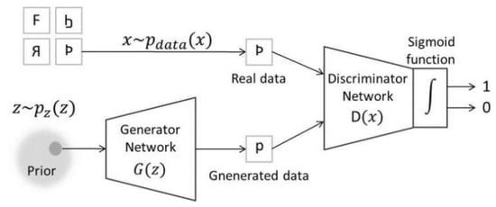
Figure 1. The schematic diagram of the generative adversarial network (GAN).

In the function ${\mathrm{V}}_{\mathrm{GAN}}(G,D)$, the first item represents the entropy of data from real distribution judged by D. D tries to maximize the result. The second item is the entropy of the data generated by G from random inputs discriminated by D. D tries to make this item bigger and equivalently minimize the $D(G(z))$ to guarantee its ability to distinguish falsehood from truth. In short, D wants to maximize the function ${\mathrm{V}}_{\mathrm{GAN}}(G,D)$. On the other hand, the task of G is completely the opposite which tries to maximize the $D(G(z))$ and minimize the function ${\mathrm{V}}_{\mathrm{GAN}}(G,D)$. This kind of training of GAN just meets the minimax two-player game of game theory.

GAN has many advantages compared with traditional ones. It can be trained only with backpropagation and there is no need for any Markov chains or unrolled approximate inference networks during either training or generation of samples [56]. What is more, the parameter updating of G is not directly from data samples, but also related to the backpropagation of D. However, the disadvantages are also obviously summarized as poor interpretability and stability. There is no explicit representation for the distribution of G, and that D must be synchronized well with G during training [56]. Nowadays, there are some improved models have been proposed to overcome these disadvantages like DCGAN [57], CGAN [58], InfoGAN [59], WGAN [60], LSGAN [61], EBGAN [62], and so on.

2.2.2. Advantages of Residual Network

In 2015, ResNet [63] has led to a series of breakthroughs in image classification and detection-whenever emergence, and became a backbone network in many computer vision tasks for feature extraction. At that time, researchers wanted to improve the accuracy of networks by deepening the layers, but the unexpected degradation or gradient vanishing appeared. Then He et al. [63] came up with the solution that constructing the new layers by identity mapping which just the core idea of ResNet. Figure 2 shows the residual block with shortcut connections.

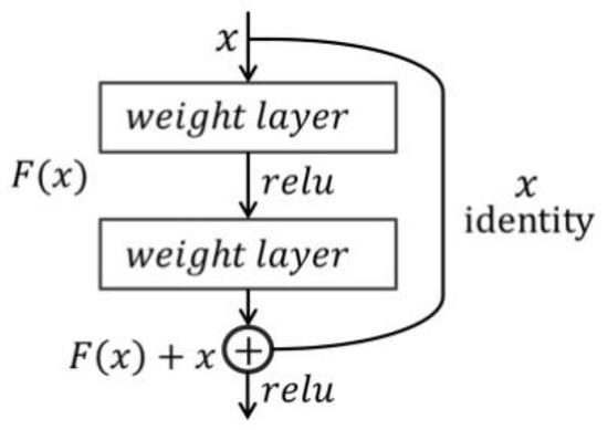
Figure 2. The residual block of a residual network (ResNet).

Each residual block contains a few stacked nonlinear layers. The input of the former layer jumps over some middle layers and is added together with the layer behind to learn an identity mapping. As we all know, if the residual $F(x)=0$, the stacked layers exactly achieve the identity mapping and the network performance will not degrade at least. Actually, the residual cannot be 0, so the stacked layers can learn new features anyhow based on input features to make the network achieve better performance. Another benefit is that the loss can transmit to former layers quickly to update the weights. All those advantages will help to promote the accuracy of networks. Some trained networks like ResNet-50, ResNet-101, ResNet-152, and so on, have been widely applied in image processing tasks.

3. Proposed Method

In the following content, details of the infrared and visible image fusion method with GAN and ResNet is be introduced. The formulation and framework will be described first, and then the designed structures of D and G are discussed, respectively. At last, we analyze the loss functions which guide the backpropagation of the networks.

3.1. The Overall Fusion Framework

As mentioned earlier, the infrared and visible image fusion is regarded as an adversarial process between G and D. The training and testing operations are not exactly the same. Only the trained G is needed when testing. The entire process is described in detail below. The training process mainly contains 4 steps. First, the infrared image I and visible image V are concatenated in the channel dimension forming a synthetic 2-channels input retaining the same height and width of the source images. Then, the input is fed to G to generate the preliminary fused image F. Meanwhile, the size and dimension of the fused image are consistent with either source image. Next, the F and V are fed to D respectively to get the discriminant probabilities belonging to (0, 1). Among them, F is the fake image whereas V is regarded as the label. Finally, the parameters of G and D are updated through backpropagation according to the loss function which will be given detail description in Section 3.3. In general, the loss of G guarantees that F contains more considerable intensity information of I and partial gradient information of V, whereas the loss of D gradually adds more visible detail to F. As to the testing process, we just need the first two steps of training, using the trained G to get the final fused image. Figure 3 shows the framework of our fusion process.

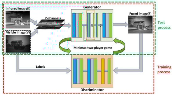
Figure 3. The framework of infrared and visible image fusion.

3.2. The Network Structures of G and D

The novel structure and scheme of G and D proposed are introduced in the following contents which play an important role in the whole realization.

3.2.1. The Structure of G

In our method, G consists of five separate convolution layers with batch-normalization (BN) layers and activation functions, two residual blocks, and two skip connections. There are two convolution layers in each of the residual blocks. These components, combined appropriately, can make the G network easy to optimize and achieve ideal outputs. The size of all convolution kernels is set to 3 × 3 except the last layer which is set to 1 × 1. All the strides are set to 1 in G to extract image features as much as possible. Considering the residual blocks in the network, all the convolution operations are implemented with padding to keep the output of each layer having the same size as the input. However, the padding will cause some undesirable gray blocks around edges in the fused image and the solution will be given in the testing process in Section 4.1.2. At the beginning of G, the two-channel concatenated images are fed to the convolution layer and 64 feature maps are then obtained which become the inputs of the residual block and the source maps of skip connection. The first convolution layer mainly extracts the basic feature maps. Inspired by Ledig et al. [64], the block layout is employed twice, and each residual block is followed by a convolution layer called the transfer layer, whose outputs are added to the source maps of the skip connection. Then, another two convolution layers are used to extract features, and at the same time, reduce the output dimensions to a single channel. The residual blocks and skip connections introduced in the generator play an important role. The network layers can be deepened by adding residual blocks which help to improve the performance of the network. The unique structure of identity mapping in the residual block can keep the integrity of its input and make it easy to learn residual information at the same time. This is important for the fusion task which can keep the feature maps of the source images extracted by former layers and anyhow learn more potential internal connections. Also, skip connections are added. The residual block, transfer layer, and the skip connection can be regarded as another “big residual block”. All of these guarantee that more useful features are generated and retained before reducing the dimensionality to a single-channel fused image. In short, the join of residual blocks and skip connections can preserve more deep features and make use of the former information of extracted maps. Also, the network is easier to optimize although some layers are added. Meanwhile, the use of BN and Leaky ReLU will help to overcome the problem of gradient vanishing and difficult training, and then improve the accuracy and the convergence speed of the model. The schematic structure of G with loss function is shown in Figure 4.

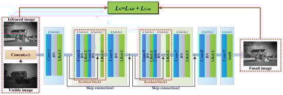
Figure 4. The network structure of the generator.

In order to make the architecture of the generator look clearer, the details are outlined in Table 1. Conv suffixed with a specified number denotes the corresponding convolution block which contains the convolution layer, BN, and Leaky ReLU, except the last convolution block. Net suffixed with a specified number denotes the output features of the corresponding convolution block. Add suffixed with a specified number denotes the add operation for residual blocks and skip connections.

Table 1. The architecture of the generator.

Name	Layer	Kernel Size	Stride	Channel (Input)	Content (Input)	Channel (Output)	Content (Output)	Padding	Activation
Input layer	Conv1	3 * 3	1	2	Image pair	64	Net1	SAME	LReLU
Residual block1	Conv2	3 * 3	1	64	Net1	64	Net2	SAME	LReLU
	Conv3	3 * 3	1	64	Net2	64	Net3	SAME	/
	Add1	/	/	/	Net1/Net3	/	Net1 + Net3	/	LReLU
Transfer layer1	Conv4	3 * 3	1	64	LReLU (Net1 + Net3)	64	Net4	SAME	LReLU
Skip connection1	Add2	/	/	/	Net1/Net4	/	Net1 + Net4	/	/
Residual block2	Conv5	3 * 3	1	64	Net1 + Net4	64	Net5	SAME	LReLU
	Conv6	3 * 3	1	64	Net5	64	Net6	SAME	/
	Add3	/	/	/	Net1 + Net4/Net6	/	Net1 + Net4 + Net6	/	LReLU
Transfer layer2	Conv7	3 * 3	1	64	LReLU(Net1 + Net4 + Net6)	64	Net7	SAME	LReLU
Skip connection2	Add4	/	/	/	Net1 + Net4/Net7	/	Net1 + Net4 + Net7	/	/
Output layer1	Conv8	3 * 3	1	64	Net1 + Net4 + Net7	32	Net8	SAME	LReLU
Output layer2	Conv9	1 * 1	1	32	Net8	1	Fused image	SAME	tanh

3.2.2. The Structure of D

As to D, we employ the block layout used by Radford et al. [57], which simply consists of four convolution layers and a linear layer. Some matrix transformations must be done before linear multiplication. Similar to G, each convolution layer except the first one is followed by a BN layer and the activation function which is Leaky ReLU. The last layer is a linear layer, which outputs the probability depending on whether the input is a fused image or a visible label. This time, we use 5 × 5 kernels in the first convolution layer and 3 × 3 kernels in other convolution layers. The strides are set to 2 without padding since D mainly behaves as a classifier. The first four convolution layers extract features and the last linear layer classifies them [26], so that the probability values of the fused image and visible image are obtained, respectively. These two values are used together to calculate the loss of D. The fusion results are better when the value of the fused image gets closer to the value of the visible image. The architecture of the discriminator is shown in Figure 5 and the details are outlined in Table 2.

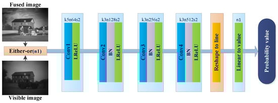
Figure 5. The network structure of discriminator.

Table 2. The architecture of the discriminator.

Layer/ Operation	Kernel Size	Stride	Channel (Input)	Content (Input)	Channel (Output)	Content (Output)	Padding	Activation
Conv1	5 * 5	2	1 (128 * 128)	Fused/ Visible image	64	Net1 (62 * 62 * 64)	VALID	LReLU
Conv2	3 * 3	2	64	Net1	128	Net2 (30 * 30 * 128)	VALID	LReLU
Conv3	3 * 3	2	128	Net2	256	Net3 (14 * 14 * 256)	VALID	LReLU
Conv4	3 * 3	2	256	Net3	512	Net4 (6 * 6 * 512)	VALID	LReLU
Change to line	/	/	/	Net4	/	Net5 (18432 * 1)	/	/
Line to value	/	/	/	Net5	/	Probability (1)	/	/

3.3. Loss Functions

The loss functions of D and G guide the optimization and we make great efforts to minimize the losses in backpropagation. The loss function of G tries to make the fused images keep the respective information of original infrared and visible images as much as possible. And the loss function of D aims to strengthen the ability to distinguish fused images from visible images. In our paper, we refer to the losses of Ledig et al. [64] and Qi et al. [61], and then design the particular loss for our method.

3.3.1. The Loss Function of G

The loss function of G($L_G$) consists of two parts which are the adversarial loss ($L_{Adv}$) and the content loss ($L_{Con}$). The calculation equation is illustrated in Equation (2):

$$L_G=L_{Adv}+L_{Con}.$$

(2)

Among them, the $L_{Adv}$ is defined as follows:

$$L_{Adv}=\frac{1}{N}{{\displaystyle {\sum }_{n=1}^N(D(F)-a)}}^2.$$

(3)

The form of mean square error (MSE) loss is used to calculate the $L_{Adv}$ and the parameter a is set approaching 1 since G wants to increase the discriminant result $D(F)$ and generate the data which cannot be distinguished by D. The smaller $L_{Adv}$ means the better-fused images generated by G.

The $L_{Con}$ is used to keep the correlations between source images and fused images, and has an influence on which kind of information will be merged from the source images in different modalities. In this paper, the structural similarity (SSIM) [65] $L_{SSIM}$ is introduced which is a kind of perceptual evaluation metric to restraint the optimization routine of the net. The $L_{SSIM}$ is the main loss since it can synthetically measure the consistency between fused image and each of input images on structure, luminance and contrast. The $L_{SSIM}$ accounts for a larger proportion in the equation. Then, the losses about image specifications are also considered which is called $L_{Grad}$. As mentioned at the beginning of the article, the intention of G is to fuse the infrared thermal radiation information of infrared image which is partly characterized by its pixel intensities [26] and the texture detail information of visible image which is partly characterized by its gradients [20]. Unlike the $L_{Adv}$, the $L_{Con}$ calculates with the image matrix. The calculation equation is illustrated in Equation (4):

$$L_{Con}={\delta }_1{L}_{SSIM}+{\delta }_2{L}_{Grad}.$$

(4)

In the $L_{SSIM}$, the SSIM between the source image and the fused image is calculated, respectively, and the weight can be adjusted to adapt to different conditions. The $L_{SSIM}$ is calculated as Equation (5):

$$L_{SSIM}=1-(\omega \cdot SSIM(A,F)+(1-\omega )\cdot SSIM(B,F)),$$

(5)

where ω represents the weight and $SSIM(*)$ just implement the structural similarity operation in [65]. A and B are source images, and F is the fused image. With the join of $L_{SSIM}$, visually pleasing fused images are always obtained, and the values are higher by objective evaluation metrics.

The $L_{Grad}$ calculates the MSE of image intensity and gradient, so the Frobenius norm is introduced to express the loss simpler. The equation of $L_{Grad}$ is organized as follows:

$$L_{Grad}=\frac{1}{HW}({\gamma }_1{\Vert F-I\Vert }_F^2+{\gamma }_2{\Vert \nabla F-\nabla V\Vert }_F^2+{\gamma }_3{\Vert F-V\Vert }_F^2+{\gamma }_4{\Vert \nabla F-\nabla I\Vert }_F^2),$$

(6)

where ${\Vert *\Vert }_F$ represents the Frobenius norm, ∇ indicates the gradient computation. H and W represent the height and weight of the input images, respectively. We innovatively employ four parameters which are ${\gamma }_1$, ${\gamma }_2$, ${\gamma }_3$, and ${\gamma }_4$ to adjust the balance of $L_{Grad}$. The first two items take up a large proportion to keep more intensity information of infrared images and gradient information of visible images. However, in a few image pairs, contrary to what we have assumed, the infrared image includes more details and the visible image has strong intensities in some regions. Therefore, the last two items are added which can synthetically improve the robustness of the model, of course, ${\gamma }_3$ is not more than ${\gamma }_1$, ${\gamma }_4$ is smaller than ${\gamma }_2$. So, the fused image generated by G will contain much information of source images.

3.3.2. The Loss Function of D

The loss function of D($L_D$) is always used to discriminate the fused image generated by G and the visible image itself. The loss consists of a positive loss and a negative loss shown as Equation (7):

$$L_D=\frac{1}{N}{\displaystyle {\sum }_{n=1}^N{(D(V)-b)}^2+}\frac{1}{N}{{\displaystyle {\sum }_{n=1}^N(D(F)-c)}}^2.$$

(7)

We all know that the texture information of visible images cannot be totally represented by their gradients, and other related information will be enriched through D. In the first item of the equation, the parameter b is set approximately to 1, since we regard V as the label and try to increase $D(V)$ to 1. On the contrary, c is close to 0. During the operation of optimizing D, we try to minimize $D(F)$, so that D always have the ability to distinguish the fake data from the true. The smaller $L_D$ means that more details of the visible image are added to the elementary fused image generated by G. The adversarial game between G and D gradually complete the fusion process that the final fused images have comprehensive information from source images.

4. Experiments and Results

4.1. Related Pre-Process and Settings

4.1.1. Data Augmentation

In our experiments, the dataset consists of 41 pairs of infrared and visible images that are collected from [66]. These image pairs mostly have evident pixel intensity in infrared images and abundant detail information in visible images. These image pairs are divided into two parts: 31 pairs for training and 10 pairs for testing. If we only use these a few dozen original images for training, it is very hard to get a stable and compatible model. So we decide to enlarge the training set by cropping source image pairs into small image blocks with certain stride. Note that, no matter the original images or the image blocks cropped, the infrared image and visible image must appear in pairs. The size of the image block is set to 128 × 128 and the stride is set to 11 in the following experiments, in consideration of the practical effect and the ability of the GPU (Graphics Processing Unit). As a result, 46,209 pairs of images are combined together as the dataset for training. The testing set consists of 10 pairs of source images that are not involved in training.

4.1.2. Training and Testing Details

As mentioned before, for training, cropped image pairs were put into G network whose batch size was set to 32 and the learning rate was initialized as ${10}^{-5}$. Our model was trained with the ADAM optimizer whose internal parameters were set as follows: ${\beta }_1=0.9$, ${\beta }_1=0.999$, $\epsilon ={10}^{-8}$. The training of G and D were time-sharing that only one network could update its weights and bias every time. As to the loss functions, the parameters a and b were vectors whose sizes were equal to the batch and randomly created within the scope of 0.7 to 1.2. We used the same way to generate the parameter c, but within the scope of 0 to 0.3. After careful analysis and experiments, the weight ω was set to 0.5, the ${\delta }_1$ was set to 1000 and the ${\delta }_2$ was set to 5, the parameters ${\gamma }_1$, ${\gamma }_2$, ${\gamma }_3$, and ${\gamma }_4$ were separately set to 15, 650, 15, and 300, respectively. The GPU platform is Intel E5-2680 V3 processor with TITAN V GPU and 64 Gb memory.

During testing, only the trained G was used to generate the fused images. When we described the structure of G earlier in the article, we have mentioned the problem of gray blocks around edges caused by convolution with padding. To get rid of these blocks, firstly, we padded the edges of the source images and the padding values were set to 6. The padding value might change according to the number of convolution layers and the actual outputs. Then we put the transformed source image pairs into G and directly got the fused images, of course, whose sizes were the same as the inputs. Then we cut out the final results from the fused imaged with the size of source images. The schematic diagram of the testing process is shown in Figure 6.

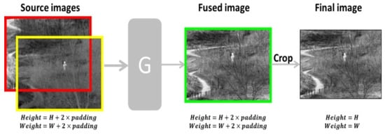
Figure 6. The image cropping of the testing process.

4.2. Objective Evaluation Metrics

In the task of infrared and visible image fusion, there is no standard reference image—the so-called ground-truth image—and it is difficult to conduct the objective evaluation. Nowadays, researchers always take a reasonable way to apply several fusion metrics to make an overall evaluation [67]. In our experiments, eight objective fusion metrics were used to evaluate the fusion results from three aspects which were the fused image itself, image correlation, and visual quality. The eight metrics were entropy (EN), spatial frequency (SF) [68], standard deviation (SD), mean structural similarity (MSSIM) [65], correlation coefficient (CC), the visual information fidelity for fusion (VIFF) [27], the sum of the correlation of differences (SCD) [69], and the feature mutual information (FMI) [70] for the discrete cosine features.

The evaluation that the larger value means the better fusion result is suitable for all eight metrics. The fused images with lager EN and SF always have more detail information and spatial frequency. The contrast of the images is reflected in SD which influences the visual attention. The MSSIM measures the mean structural similarity between the source images and fused image. It is a synthetical metric on structure, luminance, and contrast. The CC and SCD are two independent indexes for judging the amount of information transmitted from source images to the fused image. As to VIFF, it is a kind of perceptive metric based on the human visual system and the fused images are clearer and more natural with a higher VIFF. The FMI is based on information theory and measures the mutual information between image features.

All the above metrics were implemented with MATLAB using the codes by the authors or well-known third-parties. Table 3 gives the detail descriptions of the metrics used.

Table 3. The metrics for fusion evaluation.

Metrics	Formula	Description
EN	$EN = -{\displaystyle {\displaystyle \sum }_{i=0}^{255}}{p}_i{\log }_2{p}_i$	The EN can measure the information contained in the fused image. The larger EN means the better performance.
SF	$SF = \sqrt{{\left(Row\_Freq\right)}^2 + {\left(Column\_Freq\right)}^2}$ $Ro{w}_{Freq} =\sqrt{\frac{1}{MN}{\displaystyle \sum }_{j=0}^{M-1}{\displaystyle \sum }_{k=1}^{N-1}{\left[F\left(j,k\right) - F\left(j,k - 1\right)\right]}^2}$ $Colum{n}_{Freq}= \sqrt{\frac{1}{MN}{\displaystyle \sum }_{k=0}^{N-1}{\displaystyle \sum }_{j=1}^{M-1}{\left[F\left(j,k\right) - F\left(j - 1,k\right)\right]}^2}$	The SF indicates the overall activity level in an image, including the row frequency and column frequency. The fused image F will contains more detail features if the value is larger.
SD	$SD = \sqrt{\frac{1}{MN}{\displaystyle \sum }_{j=1}^M{\displaystyle \sum }_{k=1}^N{\left(F\left(j,k\right) - \mu \right)}^2}$	$\mu$ indicates the mean value of the fused image F. Generally, the larger SD means that F has high contrast and easily attracts visual attention.
MSSIM	$SSIM\left(X,F\right) = \frac{\left(2{\mu }_X{\mu }_F + C_1\right)\left(2{\sigma }_{XF} + C_2\right)}{\left({\mu }_X^2 +{\mu }_F^2 + C_1\right)\left({\sigma }_X^2 + {\sigma }_F^2 + C_2\right)}$ $MSSIM(A,B,F) = \frac{1}{2M}({\displaystyle \sum }_{j=1}^{M}SSIM(A_j,F_j) + {\displaystyle \sum }_{j=1}^{M}SSIM(B_j,F_j))$	The SSIM index is used to measure the structural similarity between source image (A or B) and fused image F. The final MSSIM uses the mean value to evaluate the overall image quality. $\mu$ denotes the mean value of the image. σ represents the standard deviation. $C_1={(k_{1}L)}^2$ and $C_2={(k_{2}L)}^2$, $k_1$ and $k_2$ are small constants much less than 1. L is the dynamic range of the pixel values (255). A larger SSIM means better fusion process.
CC	$CC = \frac{(r_{AF} + r_{BF})}{2}$ $r_{XF} = \frac{{{\displaystyle \sum }}_{i=1}^M{{\displaystyle \sum }}_{j=1}^N(X(i,j) - \overline{X})({{\displaystyle \sum }}_{i=1}^M{{\displaystyle \sum }}_{j=1}^N(F(i,j) - \mu ))}{\sqrt{{{\displaystyle \sum }}_{i=1}^M{{\displaystyle \sum }}_{j=1}^N{(X(i,j) -\overline{ X})}^2({{\displaystyle \sum }}_{i=1}^M{{\displaystyle \sum }}_{j=1}^N{(F(i,j) - \mu )}^2)}}$	$\overline{X}$ and $\mu$ represent the mean value of the source image (A or B) and the fused image F respectively. The larger CC indicates the F gains more information from the source images and the better fusion effect.
VIFF	$VIFF\left(A,B,F\right) = {\displaystyle \sum }_k{p}_k·VIF{F}_k\left(A,B,F\right)$ $VIF{F}_k\left(A,B,F\right) = \frac{{{\displaystyle \sum }}_{b}FVI{D}_{k,b}\left(A,B,F\right)}{{{\displaystyle \sum }}_{b}FVID{N}_{k,b}\left(A,B,F\right)}$	The VIFF is a multi-resolution image fusion metric using visual information fidelity (VIF) and performs better in human perception matching. The final result is determined by weighting the VIFF of each sub-band. The parameters in the Formula are complex and readers can refer to the original. The VIFF is larger when images have high visual quality.
SCD	$SCD = r_{D_{1}A }+ r_{D_{2}B}$ $D_1 = F - B\hspace{1em}\hspace{1em}{D}_{2 }= F - A$ $r_{D_{n}X} = \frac{{{\displaystyle \sum }}_{i=1}^M{{\displaystyle \sum }}_{j=1}^N\left(D_n\left(i,j\right) -\overline{ D_n}\right)({{\displaystyle \sum }}_{i=1}^M{{\displaystyle \sum }}_{j=1}^N\left(X\left(i,j\right) - \overline{X}\right))}{\sqrt{{{\displaystyle \sum }}_{i=1}^M{{\displaystyle \sum }}_{j=1}^N{\left(D_n\left(i,j\right) -\overline{ D_n}\right)}^2({{\displaystyle \sum }}_{i=1}^M{{\displaystyle \sum }}_{j=1}^N{\left(X\left(i,j\right) - \overline{X}\right)}^2)}}$	The SCD is based on the supposition that the difference between one of the input images (A) and the fused image (F) almost discloses the information transferred from the other input image (B). The opposite is also true. The value is larger when fused image contains more information from source images.
FMI	$I\left(A;F\right) = \frac{2}{n}{\displaystyle {\displaystyle \sum }_{i=1}^n}\frac{I_i\left(A;F\right)}{H_i\left(A\right)+H_i\left(F\right)} I\left(B;F\right)= \frac{2}{n}{\displaystyle {\displaystyle \sum }_{i=1}^n}\frac{I_i\left(B;F\right)}{H_i\left(B\right)+H_i\left(F\right)}$ $FM{I}_F^{AB} = \frac{1}{n}{\displaystyle \sum }_{i=1}^n(\frac{I_i\left(A;F\right)}{H_i\left(A\right)+H_i\left(F\right)} + \frac{I_i\left(B;F\right)}{H_i\left(B\right) + H_i\left(F\right)})$	The FMI calculates the mutual information of the image features using a feature extraction method extracts the feature image of the source (A) and (B) and fused images (F). $I_i\left(X;F\right)$ means the regional mutual information and $H_i\left(X\right)$ are the entropies. The larger FMI means the better achievement.

4.3. Fusion Results

In this part, nine other fusion methods are recommended to compare the fusion results with ours, including curvelet transform (CVT) [71], dual-tree complex wavelet transform (DTCWT) [72], Laplacian pyramid (LP) [73], nonsubsampled contourlet transform (NSCT) [74], two-scale image fusion based on visual saliency (TSIFVS) [75], guided filtering based fusion (GFF) [76], and convolutional neural network based fusion (CNN) [24], dense block based fusion [55] which includes Dense-add and Dense-L1 according to the different fusion strategies, and a GAN based method (FusionGAN) [26]. We used the codes provided by the authors or a well-known toolbox to generate the fused images from source image pairs except for the last method which cannot get the ideal outputs directly. The first six methods are conventional fusion methods and the last three methods are the DL-based methods proposed recently.

4.3.1. Subjective Evaluation

In order to elaborate the fusion effects of different methods clearly and have an intuitional vision experience, firstly, the fusion results obtained by different methods of six infrared and visible image pairs from the TNO database are shown in Figure 7. Moreover, two groups of single image comparisons are given, and we can easily judge the fusion quality by subjective assessment. Figure 8 and Figure 9 show the fusion results of “Marne_04” and “lake” of the TNO dataset.

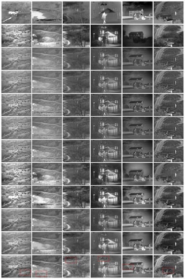
Figure 7. Fusion results of six infrared and visible image pairs. From top to bottom: infrared images, visible images, the results of curvelet transform (CVT), dual-tree complex wavelet transform (DTCWT), Laplacian pyramid (LP), nonsubsampled contourlet transform (NSCT), two-scale image fusion based on visual saliency (TSIFVS), guided filtering based fusion (GFF), convolutional neural network based fusion (CNN), Dense-add, Dense-L1, and the proposed method.

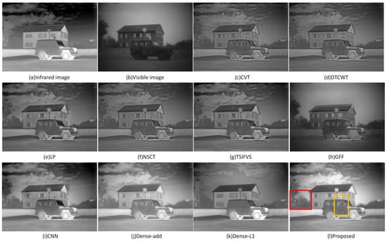
Figure 8. Fused images of “Marne_04”.

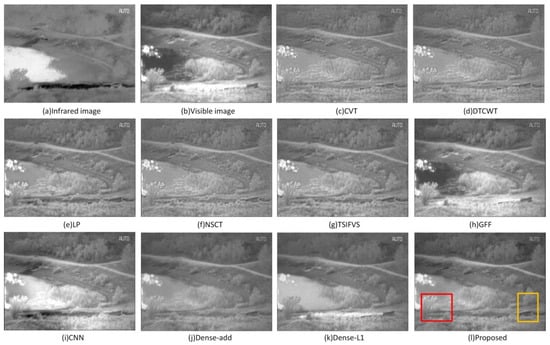
Figure 9. Fused images of “lake”.

In Figure 8, the fused images obtained by CVT, DTCWT, LP, NSCT, TSIFVS although contain the information of two source images, but are not very clear and have low contrast. The images obtained by GFF and Dense-L1 tend to approximate to just one kind source image. As to the other fused images, the image obtained by the proposed method looks smoother than the image obtained by CNN which has some undesirable regions around the eave and the front window of the jeep. The image obtained by Dense-add is good, but has a lower contrast than the image obtained by the proposed method. The gaps of branches and the spot of the jeep can be seen in the colored frames of the image obtained by the proposed method. In Figure 9, the characteristics of the fused images are similar to Figure 8. We can easily distinguish the plants, riverbank, and other objects in the colored frames of the image obtained by the proposed method.

As mentioned above, the fused images obtained by the proposed method always contain more details, and there is less noise added to the fused image which can guarantee a high correlation with source images. What is more, the results fused by our method have high visual information fidelity and look more natural and comfortable.

4.3.2. Objective Evaluation

For quantitative comparisons, we chose ten fused images from the results and evaluated them through the above-mentioned eight metrics. The results of the eight metrics are plotted in Figure 10 and the average values are listed in Table 4.

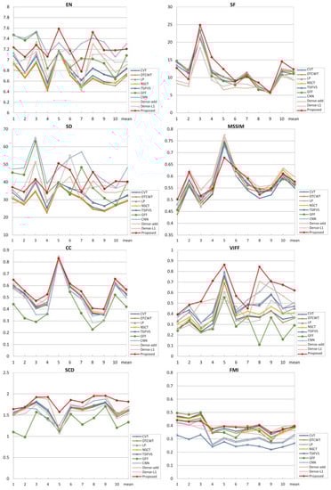
Figure 10. Quantitative values of eight metrics.

Table 4. The average values of the eight metrics on 10 fused images.

Methods	EN	SF	SD	MSSIM	CC	VIFF	SCD	FMI
CVT	6.73408	11.639	29.6285	0.5494	0.5225	0.3693	1.5916	0.3985
DTCWT	6.69775	11.5691	29.2046	0.5579	0.5265	0.3589	1.5957	0.3876
LP	6.84323	11.8508	32.7525	0.5665	0.5214	0.4518	1.612	0.33449
NSCT	6.72252	11.6472	29.6933	0.5761	0.5312	0.4084	1.614	0.38241
TSIFVS	6.83149	11	32.23	0.5749	0.5286	0.4718	1.6278	0.26754
GFF	7.08199	11.1043	40.147	0.5653	0.42	0.2913	1.3317	0.38956
CNN	7.30549	11.8958	48.1136	0.5673	0.4956	0.5067	1.622	0.32205
Dense-add	6.91024	9.23227	35.66657	0.59713	0.55035	0.49293	1.69591	0.40567
Dense-L1	6.96276	9.31077	38.90169	0.57984	0.51258	0.3619	1.53546	0.36227
FusionGAN	7.3033	6.4600	51.9542	0.3352	0.7646	0.5213	−	−
Proposed	7.20581	12.3369	40.18583	0.57658	0.56588	0.6208	1.81625	0.39641

In Table 4, The values in italic of FusionGAN [26] are not calculated by the authors and they are cited from the original article for reference. Among other values in the table, the best values for each metric are in bold. The proposed method gets the four best values in SF, CC, VIFF, and SCD, also all other metrics are in the top three places, respectively. On the whole, we can further summarize that the proposed fusion method has obvious advantages in getting detailed information from source images and keeping the correlation with source images. Especially, the VIFF index is more salient than others, since the generator is designed with ResNet and skip connections. Also, the loss functions proposed have made appropriate constraints for optimization.

Firstly, we compare the results with the original FusionGAN [26]. Since we cannot get normal fused results like the images cited in the article from the codes and the trained model provided by the authors, we just use the average values calculated in their article where the source image pairs are mainly consistent with the proposed method. The values may be regarded as a reference, but we cannot make sure whether the source codes of the metrics are the same or not with ours. So we can make an intuitive observation of the images in the article and the proposed method. It is easy to find that the fused image of the proposed method looks more natural and clear, mainly because of the adjustments of the network and loss functions.

Next, the values of other conventional methods and DL-based methods are compared with the proposed method. From the results shown in Table 4 and Figure 10, we can see that DL-based methods can get commendable achievements in infrared and visible image fusion. The largest SF indicates that the images fused by the proposed method contain more detailed textures. The best value of CC and SCD means that our fused images are highly correlated with the source images. What is more, the proposed method gets the largest value in VIFF which means that visual information is kept as much as possible. This revalidates the conclusion drawn by the subjective evaluation that our fused images look more natural and clearer. The method based on CNN is better than the proposed method in the metrics of EN and SD, so the fused images always have higher contrast which can easily attract people’s attention. The method not only generates the weight maps based on CNN, but also combines the multi-scale transforms, which helped a lot. The method based on Dense-add gets the best values in MSSIM and FMI, probably because the network of Dense-add contains dense blocks that can preserve as much information as possible obtained by each middle layer. The SSIM loss is also used in the Dense-add when training. The proposed method is a little weak in SD and MSSIM, and we will try our best to complement the shortages by optimizing the structure and the loss functions hereafter.

Taken together, our fusion model can get the best performance among these methods. At the same time, there are no complicated transforms and pre-training needed, which can reduce the computational cost and complexity.

4.4. Model Analyses

Our fusion method with GAN and ResNet is a DL-based method that is distinct from traditional ones. Most traditional methods like MSD based, SR based, or others, directly make pixel-level operations on source images and somehow can establish the correlations between the source image and fused image easily. However, our DL-based generative model needs to generate the image through weights and bias of the network which are different to train. The structures of G and D may have a great influence on fusion results. In addition, the loss functions of G and D together determine the optimization strategies and what kinds of information will be added to the final image. So the design of loss functions is another troublesome problem.

In order to solve these difficulties, firstly, we refer to the mature models of [57,64], and construct the networks of our fusion model with GAN and ResNet. The residual blocks, skip connections, convolution layers, and BN layers work together for feature extraction and combination. The network designed for fusion is other than classification and there is no pooling operation, which may cause the loss of image information. Not only the original residual blocks are introduced, but also the “big residual blocks” are designed. They work together to guarantee that more useful features are generated and retained before reducing the dimensionality to a single-channel fused image. Meanwhile, the ADAM optimizer is adopted with proper settings. Furthermore, the loss function of G in our method consists of adversarial loss and the content loss, which help to increase the intensities of infrared image and the texture details of the visible image. The loss function of D which judges the label image and the image generated by G makes further efforts to add information from visible images.

5. Conclusions

In this paper, we proposed an infrared and visible image fusion method with GAN and ResNet. This is an end-to-end model and no pre-training is needed. The G network generates the elementary images with infrared thermal radiation information and visible texture information and D gradually adds more details of visible image to the final results. The join and combination of residual blocks and skip connections can extract and reserve more features which are important for the fusion task. At the same time, they can promote the flexibility and non-linear capability of G and help to optimize the parameters in backpropagation. The loss functions designed with adversarial loss and content loss behave well which conduct the fusion tendency and information contained in the fused images. The results of subjective and objective evaluations indicate that the images fused by the proposed method contain more details and they are highly correlated with the source images. In particular, the visual information fidelity of the fused images is more prominent than other methods and makes the images better for human perception matching.

We believe that the basic framework of our fusion method can be applied to other image fusion tasks, such as medical image fusion, multi-exposure image fusion, and multi-focus image fusion with some changes in the loss functions and labels.

References

- Goshtasby, A.A.; Nikolov, S. Image fusion: Advances in the state of the art. Inf. Fusion 2007, 8, 114–118. [Google Scholar] [CrossRef]
- Li, H.; Wu, X.J.; Kittler, J. Infrared and Visible Image Fusion using a Deep Learning Framework. In Proceedings of the 2018 24th International Conference on Pattern Recognition (ICPR), Beijing, China, 20–24 August 2018. [Google Scholar]
- Reinhard, E.; Ashikmin, M.; Gooch, B.; Shrley, P. Color transfer between images. IEEE Comput. Graph. Appl. 2002, 21, 34–41. [Google Scholar] [CrossRef]
- Kumar, P.; Mittal, A.; Kumar, P. Fusion of Thermal Infrared and Visible Spectrum Video for Robust Surveillance. In Proceedings of the Computer Vision, Graphics and Image Processing, 5th Indian Conference, ICVGIP 2006, Madurai, India, 13–16 December 2006. [Google Scholar]
- Simone, G.; Farina, A.; Morabito, F.C.; Serpico, S.B.; Bruzzone, L. Image fusion techniques for remote sensing applications. Inf. Fusion 2002, 3, 3–15. [Google Scholar] [CrossRef]
- Ma, J.; Ma, Y.; Li, C. Infrared and visible image fusion methods and applications: A survey. Inf. Fusion 2018, 45, 153–178. [Google Scholar] [CrossRef]
- Li, S.; Yang, B.; Hu, J. Performance comparison of different multi-resolution transforms for image fusion. Inf. Fusion 2011, 12, 74–84. [Google Scholar] [CrossRef]
- Pajares, G.; Cruz, J.M.D.L. A wavelet-based image fusion tutorial. Pattern Recognit. 2004, 37, 1855–1872. [Google Scholar] [CrossRef]
- Zhong, Z.; Blum, R.S. A categorization of multiscale-decomposition-based image fusion schemes with a performance study for a digital camera application. Proc. IEEE 1999, 87, 1315–1326. [Google Scholar] [CrossRef]
- Wang, J.; Peng, J.; Feng, X.; He, G.; Fan, J. Fusion method for infrared and visible images by using non-negative sparse representation. Infrared Phys. Technol. 2014, 67, 477–489. [Google Scholar] [CrossRef]
- Li, S.; Yin, H.; Fang, L. Group-Sparse Representation With Dictionary Learning for Medical Image Denoising and Fusion. ITBE 2012, 59, 3450–3459. [Google Scholar] [CrossRef]
- Xiang, T.; Yan, L.; Gao, R. A fusion algorithm for infrared and visible images based on adaptive dual-channel unit-linking PCNN in NSCT domain. Infrared Phys. Technol. 2015, 69, 53–61. [Google Scholar] [CrossRef]
- Kong, W.; Zhang, L.; Lei, Y. Novel fusion method for visible light and infrared images based on NSST–SF–PCNN. Infrared Phys. Technol. 2014, 65, 103–112. [Google Scholar] [CrossRef]
- Bavirisetti, D.P. Multi-sensor Image Fusion based on Fourth Order Partial Differential Equations. In Proceedings of the 20th International Conference on Information Fusion (Fusion), Xi’an, China, 10–13 July 2017. [Google Scholar]
- Kong, W.; Lei, Y.; Zhao, H. Adaptive fusion method of visible light and infrared images based on non-subsampled shearlet transform and fast non-negative matrix factorization. Infrared Phys. Technol. 2014, 67, 161–172. [Google Scholar] [CrossRef]
- Xiaoye, Z.; Yong, M.; Fan, F.; Ying, Z.; Jun, H. Infrared and visible image fusion via saliency analysis and local edge-preserving multi-scale decomposition. J. Opt. Soc. Am. A 2017, 34, 1400–1410. [Google Scholar]
- Zhao, J.; Chen, Y.; Feng, H.; Xu, Z.; Li, Q. Infrared image enhancement through saliency feature analysis based on multi-scale decomposition. Infrared Phys. Technol. 2014, 62, 86–93. [Google Scholar] [CrossRef]
- Yu, L.; Liu, S.; Wang, Z. A general frame work for image fusion based on multi-scale transform and sparse representation. Inf. Fusion 2015, 24, 147–164. [Google Scholar]
- Ma, J.; Zhou, Z.; Wang, B.; Zong, H. Infrared and visible image fusion based on visual saliency map and weighted least square optimization. Infrared Phys. Technol. 2017, 82, 8–17. [Google Scholar] [CrossRef]
- Ma, J.; Chen, C.; Li, C.; Huang, J. Infrared and visible image fusion via gradient transfer and total variation minimization. Inf. Fusion 2016, 31, 100–109. [Google Scholar] [CrossRef]
- Zhao, J.; Cui, G.; Gong, X.; Zang, Y.; Tao, S.; Wang, D. Fusion of visible and infrared images using global entropy and gradient constrained regularization. Infrared Phys. Technol. 2017, 81, 201–209. [Google Scholar] [CrossRef]
- Yu, L.; Xun, C.; Wang, Z.; Wang, Z.J.; Wang, X. Deep learning for pixel-level image fusion: Recent advances and future prospects. Inf. Fusion 2018, 42, 158–173. [Google Scholar]
- Liu, Y.; Chen, X.; Peng, H.; Wang, Z. Multi-focus image fusion with a deep convolutional neural network. Inf. Fusion 2017, 36, 191–207. [Google Scholar] [CrossRef]
- Liu, Y.; Chen, X.; Cheng, J.; Peng, H.; Wang, Z. Infrared and visible image fusion with convolutional neural networks. Int. J. Wavelets Multiresolution Inf. Process. 2018, 16, 1850018. [Google Scholar] [CrossRef]
- Li, H.; Wu, X.J. Infrared and Visible Image Fusion with ResNet and zero-phase component analysis. Infrared Phys. Technol. 2018, 102, 103039. [Google Scholar] [CrossRef]
- Jiayi, M.; Wei, Y.; Pengwei, L.; Chang, L.; Junjun, J. FusionGAN: A generative adversarial network for infrared and visible image fusion. Inf. Fusion 2018, 48, 11–26. [Google Scholar]
- Han, Y.; Cai, Y.; Cao, Y.; Xu, X. A new image fusion performance metric based on visual information fidelity. Inf. Fusion 2013, 14, 127–135. [Google Scholar] [CrossRef]
- Vanmali, A.V.; Gadre, V.M. Visible and NIR image fusion using weight-map-guided Laplacian–Gaussian pyramid for improving scene visibility. Sadha 2017, 42, 1063–1082. [Google Scholar] [CrossRef]
- Liu, Z.; Tsukada, K.; Hanasaki, K.; Ho, Y.K.; Dai, Y.P. Image fusion by using steerable pyramid. PaReL 2001, 22, 929–939. [Google Scholar] [CrossRef]
- Jin, H.; Wang, Y. A fusion method for visible and infrared images based on contrast pyramid with teaching learning based optimization. Infrared Phys. Technol. 2014, 64, 134–142. [Google Scholar] [CrossRef]
- Zou, Y.; Liang, X.; Wang, T. Visible and Infrared Image Fusion Using the Lifting Wavelet. Telkomnika Indones. J. Electr. Eng. 2013, 11, 6290–6295. [Google Scholar] [CrossRef]
- Yan, X.; Qin, H.; Li, J.; Zhou, H.; Zong, J.-G. Infrared and visible image fusion with spectral graph wavelet transform. J. Opt. Soc. Am. A Opt. Image Sci. Vis. 2015, 32, 1643–1652. [Google Scholar] [CrossRef]
- Zhang, Z.; Liang, X.; Du, J. Infrared-visible video fusion based on motion-compensated wavelet transforms. IET Image Process. 2015, 9, 318–328. [Google Scholar]
- Meng, F.; Song, M.; Guo, B.; Shi, R.; Shan, D. Image fusion based on object region detection and Non-Subsampled Contourlet Transform. Comput. Electr. Eng. 2017, 62, 375–383. [Google Scholar] [CrossRef]
- Adu, J.H.; Wang, M.H.; Wu, Z.Y.; Hu, J. Infrared Image and Visible Light Image Fusion Based on Nonsubsampled Contourlet Transform and the Gradient of Uniformity. Int. J. Adv. Comput. Technol. 2012, 8009, 1309–1311. [Google Scholar]
- Olshausen, B.A.; Field, D.J. Emergence of simple-cell receptive field properties by learning a sparse code for natural images. Nature 1996, 381, 607–609. [Google Scholar] [CrossRef] [PubMed]
- Li, S.; Kang, X.; Fang, L.; Hu, J.; Yin, H. Pixel-level image fusion: A survey of the state of the art. Inf. Fusion 2016, 33, 100–112. [Google Scholar] [CrossRef]
- Yin, H.; Li, S. Multimodal image fusion with joint sparsity model. OPTEN 2011, 50, 7007. [Google Scholar] [CrossRef]
- Zhang, Q.; Liu, Y.; Blum, R.S.; Han, J.; Tao, D. Sparse Representation based Multi-sensor Image Fusion for Multi-focus and Multi-modality Images: A Review. Inf. Fusion 2017, 40, 57–75. [Google Scholar] [CrossRef]
- Hong, J.; Tian, Y. Fuzzy image fusion based on modified Self-Generating Neural Network. Expert Syst. Appl. 2011, 38, 8515–8523. [Google Scholar]
- Eckhorn, R.; Reitboeck, H.J.; Arndt, M.; Dicke, P.W. A neural network for feature linking via synchronous activity. Can. J. Microbiol. 1989, 46, 759–763. [Google Scholar]
- Li, S.; Yang, B. Hybrid Multiresolution Method for Multisensor Multimodal Image Fusion. IEEE Sens. J. 2010, 10, 1519–1526. [Google Scholar]
- Li, S.; Yang, B. Multifocus image fusion by combining curvelet and wavelet transform. Pattern Recognit. Lett. 2008, 29, 1295–1301. [Google Scholar] [CrossRef]
- Liu, Z.; Yin, H.; Fang, B.; Chai, Y. A novel fusion scheme for visible and infrared images based on compressive sensing. Opt. Commun. 2015, 335, 168–177. [Google Scholar] [CrossRef]
- Zhang, Q.; Maldague, X. An infrared-visible image fusion scheme based on NSCT and compressed sensing. In Proceedings of the Signal Processing, Sensor/Information Fusion, and Target Recognition XXIV, Baltimore, MD, USA, 20–24 April 2015. [Google Scholar]
- Wang, Z.; Gong, C. A multi-faceted adaptive image fusion algorithm using a multi-wavelet-based matching measure in the PCNN domain. Appl. Soft Comput. 2017, 61, 1113–1124. [Google Scholar] [CrossRef]
- Lin, Y.; Song, L.; Zhou, X.; Huang, Y. Infrared and visible image fusion algorithm based on Contourlet transform and PCNN. In Proceedings of the Infrared Materials, Devices, and Applications, Beijing, China, 11–15 November 2007. [Google Scholar]
- Yin, M.; Duan, P.; Liu, W.; Liang, X. A novel infrared and visible image fusion algorithm based on shift-invariant dual-tree complex shearlet transform and sparse representation. Neurocomputing 2017, 226, 182–191. [Google Scholar] [CrossRef]
- Yin, H.; Liu, Z.; Fang, B.; Li, Y. A novel image fusion approach based on compressive sensing. Opt. Commun. 2015, 354, 299–313. [Google Scholar] [CrossRef]
- Tu, T.M.; Su, S.-C.; Shyu, H.-C.; Huang, P.S. A new look at IHS-like image fusion methods. Inf. Fusion 2001, 2, 177–186. [Google Scholar] [CrossRef]
- Rahmani, S.; Strait, M.; Merkurjev, D.; Moeller, M.; Wittman, T. An Adaptive IHS Pan-Sharpening Method. IEEE Geosci. Remote Sens. Lett. 2010, 7, 746–750. [Google Scholar] [CrossRef]
- Chandra Mouli, P.V.S.S.R.; Rajkumar, S. Infrared and Visible Image Fusion Using Entropy and Neuro-Fuzzy Concepts; ICT and Critical Infrastructure: 48th Annual Convention of CSI; Springer: Cham, Switzerland, 2014. [Google Scholar]
- Mitianoudis, N.; Stathaki, T. Pixel-based and region-based image fusion schemes using ICA bases. Inf. Fusion 2007, 8, 131–142. [Google Scholar] [CrossRef]
- Simonyan, K.; Zisserman, A. Very Deep Convolutional Networks for Large-Scale Image Recognition. arXiv 2015, arXiv:1409.1556. [Google Scholar]
- Li, H.; Wu, X.-J. DenseFuse: A Fusion Approach to Infrared and Visible Images. ITIP 2019, 28, 2614–2623. [Google Scholar] [CrossRef]
- Goodfellow, I.J.; Pouget-Abadie, J.; Mirza, M.; Bing, X.; Warde-Farley, D.; Ozair, S.; Courville, A.; Bengio, Y. Generative Adversarial Nets. Proc. 27th Int. Conf. Neural Inf. Process. Syst. 2014, 2, 2672–2680. [Google Scholar]
- Radford, A.; Metz, L.; Chintala, S. Unsupervised Representation Learning with Deep Convolutional Generative adversarial Networks. Comput. Sci. 2015, 1511, 6434. [Google Scholar]
- Mirza, M.; Osindero, S. Conditional generative adversarial nets. Comput. Sci. 2014, 2672–2680. [Google Scholar]
- Chen, X.; Duan, Y.; Houthooft, R.; Schulman, J.; Sutskever, I.; Abbeel, P. InfoGAN: Interpretable Representation Learning by Information Maximizing Generative Adversarial Nets. In Neural Information Processing Systems; ACM: Barcelona, Spain, 2016. [Google Scholar]
- Arjovsky, M.; Chintala, S.; Bottou, L. Wasserstein Generative Adversarial Networks. In Proceedings of the International conference on machine learning, Vancouver, BC, Canada; 2017; Volume 70, pp. 214–223. [Google Scholar]
- Qi, G. Losssensitive generative adversarial networks on lipschitz densities. Int. J. Comput. Vis. 2019, 1–23. [Google Scholar]
- Zhao, J.; Mathieu, M.; Lecun, Y. Energy-based Generative Adversarial Network. arXiv 2016, arXiv:1609.03126. [Google Scholar]
- He, K.; Zhang, X.; Ren, S.; Jian, S. Deep Residual Learning for Image Recognition. In Proceedings of the 2016 IEEE Conference on Computer Vision and Pattern Recognition (CVPR), Las Vegas, NV, USA, 27–30 June 2016; pp. 770–778. [Google Scholar]
- Ledig, C.; Theis, L.; Huszar, F.; Caballero, J.; Cunningham, A.; Acosta, A.; Aitken, A.; Tejani, A.; Totz, J.; Wang, Z. Photo-Realistic Single Image Super-Resolution Using a Generative Adversarial Network. In Proceedings of the IEEE Conference on Computer Vision and Pattern Recognition, Honolulu, HI, USA, 21–26 July 2017. [Google Scholar]
- Wang, Z.; Bovik, A.C.; Sheikh, H.R.; Simoncelli, E.P. Image Quality Assessment: From Error Visibility to Structural Similarity. IEEE Trans. Image Process. 2004, 13, 600–612. [Google Scholar] [CrossRef]
- Alexander, T. TNO Image Fusion Dataset. Available online: https://figshare.com/articles/TNImageFusionDataset/1008029 (accessed on 26 April 2014).
- Liu, Z.; Blasch, E.; Xue, Z.; Zhao, J.; Laganiere, R.; Wu, W. Objective Assessment of Multiresolution Image Fusion Algorithms for Context Enhancement in Night Vision: A Comparative Study. IEEE Trans. Pattern Anal. Mach. Intell. 2011, 34, 94–109. [Google Scholar] [CrossRef]
- Eskicioglu, A.M.; Fisher, P.S. Image quality measures and their performance. IEEE Trans. Commun. 1995, 43, 2959–2965. [Google Scholar] [CrossRef]
- Aslantas, V.; Bendes, E. A new image quality metric for image fusion: The sum of the correlations of differences. AEU Int. J. Electron. Commun. 2015, 69, 1890–1896. [Google Scholar] [CrossRef]
- Haghighat, M.; Razian, A. Masoud Fast-FMI: Non-reference image fusion metric. In Proceedings of the 2014 IEEE 8th International Conference on Application of Information and Communication Technologies (AICT), Astana, Kazakhstan, 15–17 Octorber 2014; pp. 1–3. [Google Scholar]
- Nencini, F.; Garzelli, A.; Baronti, S.; Alparone, L. Remote sensing image fusion using the curvelet transform. Inf. Fusion 2007, 8, 143–156. [Google Scholar] [CrossRef]
- Lewis, J.J.; O’Callaghan, R.J.; Nikolov, S.G.; Bull, D.R.; Canagarajah, N. Pixel-and region-based image fusion with complex wavelets. Inf. Fusion 2007, 8, 119–130. [Google Scholar] [CrossRef]
- Burt, P.J.; Adelson, E.H. The Laplacian pyramid as a compact image code. IEEE Trans. Commun. 1983, 31, 532–540. [Google Scholar] [CrossRef]
- Zhang, Q.; Guo, B.-l. Multifocus image fusion using the nonsubsampled contourlet transform. SIGPR 2009, 89, 1334–1346. [Google Scholar] [CrossRef]
- Bavirisetti, D.P.; Dhuli, R. Two-scale image fusion of visible and infrared images using saliency detection. Infrared Phys. Technol. 2016, 76, 52–64. [Google Scholar] [CrossRef]
- Li, S.; Kang, X.; Hu, J. Image Fusion with Guided Filtering. ITIP 2013, 22, 2864–2875. [Google Scholar]
© 2020 by the authors. Licensee MDPI, Basel, Switzerland. This article is an open access article distributed under the terms and conditions of the Creative Commons Attribution (CC BY) license (http://creativecommons.org/licenses/by/4.0/).