Traffic Measurement and Congestion Detection Based on Real-Time Highway Video Data

Abstract

Since global road traffic is steadily increasing, the need for intelligent traffic management and observation systems is becoming an important and critical aspect of modern traffic analysis. In this paper, we cover the development and evaluation of a traffic measurement system for tracking, counting and classifying different vehicle types based on real-time input data from ordinary highway cameras by using a hybrid approach including computer vision and machine learning techniques. Moreover, due to the relatively low framerate of such cameras, we also present a prediction model to estimate driving paths based on previous detections. We evaluate the proposed system with respect to different real-life road situations including highway-, toll station- and bridge-cameras and manage to keep the error rate of lost vehicles under 10%.

1. Introduction

To develop a suitable traffic management or surveillance system the current traffic on the road in a specific area has to be identified and measured respectively. There are several traffic measurement systems already in use providing data about the current traffic situation. However, such systems are typically inflexible in terms of accurate positioning in newly formed traffic hotspots. As an example, induction loops are built into the road directly where each vehicle driving on this induction loop is counted accordingly. Such induction loops are quite costly when large areas are covered (depending on the desired objective). Furthermore, repositioning is impossible, hence induction loops are difficult to modify once they are encased in the street.

Contemporary camera systems in combination with appropriate software for data use offer new ways of traffic measurement implementations. In principle, camera systems can be placed somewhat arbitrarily (depending on existing infrastructure to mount the cameras) on the road establishing a more versatile and cost effective approach for traffic measurements. To develop a camera-based traffic measurement system which is capable of tracking, counting and classification of different vehicle types, a computer system has to analyze video frames using common computer vision and machine learning techniques in a hybrid application.

The primary goal of the proposed traffic measurement system is to generate additional data for a congestion detection system. Measuring traffic with a camera-based solution has the great benefit of using already installed road surveillance cameras by public organizations. Additionally, if there are no camera systems available for a specific point of interest, such devices are easy to install as well. These cameras can usually be accessed remotely, hence it affords processing video streams from a centralized computer system. It also allows changes between common traffic hotspots in seconds by simply switching the input stream to another camera.

The success of such a system mainly depends on five identified factors following the approach of using remote cameras:

• The view angle is influencing perspective, size and driving direction of vehicles
• Image quality changes per camera due to qualitatively different camera systems
• Bandwith restrictions of installations influence both image quality and frame rate of the video feed
• The environment itself vastly changes over time with day and night cycles as well as weather conditions affecting visibility
• The traffic itself underlies variation concerning the speed, amount and direction of vehicles

This paper presents a system which is capable of dealing with the difficulties and problems stated previously. In particular, low frame rate scenarios are of special interest and need to be dealt with accordingly, since the current predominant sources of video material for traffic monitoring are susceptible to that property. A prediction model is established to enrich the raw video data with additional information. It tries to find associations between the current and past detected vehicles in order to derive driving paths.

The contributions of this work are structured as follows: A related work section gives an overview of state-of-the-art patterns and algorithms concerning computer vision and machine learning useful to the envisioned system. Furthermore, deployment scenarios from other sources similar to the proposed system are presented. The approach section describes the core architecture of the designed tracking and counting system and gives detailed insights into the actual implementation. A system evaluation section concludes the research and determines the robustness of the system under certain conditions and environments in real-world scenarios. A final conclusion and remarks about the system are given in the last section in order to provide a base for discussion, further research and future system revisions.

2. Related Work

2.1. Object Detection

2.1.1. Thresholding

According to Pal [1], thresholding is one of the eldest, simplest and most popular techniques for image segmentation. In general, this task can be categorized into two schemes: global and local thresholding. On the one hand, if there is only one threshold used for the entire image it is called global thresholding. On the other hand, if there are several subregions in an image and for each of them a different threshold is used, it is referred to as local thresholding or adaptive thresholding.

A prerequisite proposed by Haralick and Shapiro [2] is that the image must include a bright object against a dark background or vice versa. All pixel values smaller or equal to the threshold value are assigned to one cluster and the remaining ones to the other group. A simple approach of a threshold selection can either be via user input, i.e., with a range slider or automatically determined by the system itself through analysing the image beforehand [3]. This can be done by determining the corresponding histogram of the image and placing the threshold in the valley between the two modes.

As presented by Chang [4] and Moon [5], thresholding is often used as an initial segmentation step, e.g., for detecting vehicles in low-light conditions. Several approaches exists where thresholding is used to extract vertical edges at nighttime using stereo vision. Furthermore, it can also be employed for localizing taillights on grey-scale images. Hence, knowing the relations between a detected pair of taillights and, with further assumptions, the typical width of a vehicle, a 3-D range information can be inferred.

2.1.2. Edge Detection

In [6], Kenneth Dawson-Howe developed edge detection for grey-scale images because color information is not required. In principal, edges are locations where brightness changes abruptly, i.e., from white to dark or vice versa. An edge pixel has a gradient which is the rate of change and a direction or orientation. In most cases the direction is considered to be the direction of the largest growth. Moreover, Pal [1] suggests that efficient edge detection is primarily based on good detection ability (low probability of wrongly marking non-edge points), localization (edge points located as close as possible the center of true edges) and providing a single response to a single edge point.

According to Dawson [6] edge detection is typically performed using either the first or the second derivate operators. Additionally, it is also possible to combine both functions. However, to get the local maximum on the edge—this is where the rate of change is highest—the first derivate is used. The second derivate results in the zero-crossing on the edge. Pal [1] describes different kind of operators, with some of the most famous and commonly used ones being the Sobel gradient, the Prewitt gradient and the Laplace operator.

Edge detection is used as an underlying technology for a robust shape detection algorithm for two dimensional objects, as stated by Moon et al. [7]. Boundary shape information such as rectangular shapes of vehicles are important indicators for recognition tasks in aerial imagery. Hence, edge detection is often used for such a purpose due to the fact that borders can be established easily. Furthermore, clustering multiple edges is needed to form rectangular shapes to finally detect vehicles. For the presented example dealing with vehicle detection four linearly elongated edge operators are used, each for one of the four sides of the vehicle.

Another example is presented by Wu et al. in [8], where the edge detection technique is used to obtain an edge set for each candidate text area of road signs. Based on this initial areas, further processing and clustering can be made to achieve the overall goal of detecting text on road signs. Furthermore, the proposed application can be used for, e.g., driving assistant systems.

2.1.3. Background Substraction

As depicted by Brutzer at al. in [9], one of the key techniques for automatic video analysis is background subtraction, especially in the domain of video surveillance. The goal is to distinguish between foreground and background areas in video sequences using a background model.

The main task of a background subtraction method is to compare an input frame against a background model [10]. This model describes the static background area of the image. Depending on the used methodology the model consists of different kind of features. After establishing a background model each input frame is subtracted by the static background model. This subtraction is also referred to as foreground detection. Basically it is a determination of areas belonging to the foreground class resulting in a binary foreground mask. However, in order to cope with several challenges regarding real world scenarios, post-processing steps such as filtering or refining the foreground mask needs to be performed. Based on the system requirements all other processing steps, such as labelling or counting detected regions, can be built upon the background subtraction task. Figure 1 illustrates the typical background subtraction process, i.e., for a video surveillance task.

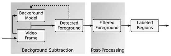
Figure 1. Typical background subtraction process with additional post-processing steps [9].

Due to the nature of video sequences background subtraction algorithms have to cope with several challenges. Some issues depicted by Brutzer [9] include gradual/sudden illumination changes, dynamic background, camouflage, shadows and video noise. To overcome challenges as mentioned before several background models have evolved. These models are explained in more detail in the subsequent sections:

• Static Background image
  According to Dawson [6], one of the simplest approaches to the background model is to pick a static frame of the video and hope that there are no moving objects inside. In the video surveillance field it is often a common technique due to the fact that these videos start with a completely static scene. Nevertheless, the drawback of this method is that it cannot deal with illumination changes. Thus, even minor changes in camera or object position problems as well as the addiction or removal of objects from the static scene.
• Frame Difference
  Frame differencing is another straightforward method that subtracts one frame from another frame as depicted by Bradski et al. in [11]. Furthermore, it is also possible to subtract from several frames later. In [6], this method eliminates the issue of needing a (static) background image to be updated. The difference for moving objects is dependent on the amount of moving and the appearance of objects in the scene. Nonetheless, it is quite difficult to analyse such image differences.
• Running Average
  Conforming to [11], this attempt is used to incorporate background changes to the model. Based on the algorithm the running average method uses a certain number of last frames to generate an update for the background model accordingly. To control the amount of change with which the background model gets updated, there is a learning rate which has to be set. For example, if the application should update its background model slowly, the used frames for averaging are set to a high value and the learning rate to a low value. Stated in [12], the running average uses the complete image for calculating the new background model. This means that it also integrates moving objects to the model. Hence, suitable parameters for this method have to be found in order to overcome this issue.
• Selectivity
  A simple way to overcome the problem of including moving objects to the background model is described in [6]. It only updates points which are determined to be background. However, this introduces another issue, namely that the knowledge is given which points belong to the background or to the foreground. To overcome this problem there is a simple comparison with the existing background model. With this additional step, objects entering but remain the scene can never become a part of the background model.
• Running Gaussian Average
  According to [12] the values of pixels change slightly from frame to frame. This is due to the nature of real world imagery scenes such as different lighting conditions, etc. However, there are also a wide variety of other factors such as the digitalization process itself which produces errors. It is often referred to real world noise and can be measured using a Gaussian distribution. If pixel values differ in more than a certain value over the standard deviation from the average they are considered to be the foreground.
• Gaussian Mixture Model
  Another issue which has to be dealt with according to [11] are background objects that move slightly, such as ripples on water, trees or grass moving in the wind, clouds traversing the sky, etc. To overcome this problem a method was proposed that models each point of the background using a mixture of Gaussian distributions. Typically, three or four distributions are adopted for each pixel. For example, in a single pixel a leave of a tree moving slightly by the wind often reveals the blue sky in the background. Hence, two of the distributions would model this pixel representing the leaf and the sky, respectively. As mentioned in [6], the basic idea is to fit multiple Gaussian distributions to the historical pixel data for each point including both foreground and background values. Each frame and each Gaussian distribution has its own weighting depending on how frequently it has occurred in the past frames. For every new frame each point is compared to the Gaussian distributions currently available in order to determine a single close Gaussian. Close Gaussian is considered to be within 2.5 times of the standard deviation from the average value. However, if nothing is found a new distribution is initialized for this point. In contrast, if a close distribution is detected it gets updated accordingly. The identified, summed up Gaussian distribution are classified to be the background if reaching a specific value.

Conforming to Dawson [6], the Gaussian Mixture Model is considered to be the standard method for modelling the background although there are newer and more complex methods in existence. It is often used as a benchmark for other background modelling techniques.

2.2. Object Recognition

2.2.1. Template Matching

This object recognition technique is widely used in machine vision for the purposes of inspection, registration and manipulation as stated by Lowe in [13]. Template matching is very effective for predefined environments where the object position and illumination are tightly controlled. However, this approach is ineffective or computationally infeasible when the object is rotated, scaled, is partially invisible or the illumination varies a lot.

According to Brunelli [14], a template is referred to as anything shaped or designed to serve as a model for a special purpose. The term matching describes the tasks of comparing something in respect to its similarity, i.e., to examine the difference between a template and the extracted snippet.

From a more algorithmic viewpoint template matching is a very simple technique where a sub-image is searched within a given image. The sub-image is typically some object of interest [6].

Conforming to Bradski [11], there are several methods to calculate an indicator in order to measure how similar two images are which is then internally used by the template matching process. The used methods are highly depending on the area of operation. The most prominent ones are the square difference matching, correlation matching and correlation coefficient matching.

Jolly at al. presented an algorithm in [15] for vehicle segmentation and classification applying deformable templates. The algorithm was used to both segment the vehicle from a complex background or from other moving vehicles in an image sequence. By defining a polygonal template to characterize a general model of a vehicle they could detect vehicles with different shapes by adjusting the template parameters.

A different approach for vehicle detection is used by Ozbay and Ercelebi [16]. Through recognizing and reading the license plate on cars and trucks it was possible to identify vehicles uniquely. After locating and segmenting the license plate and their characters, template matching is then used for classifying each of the characters.

2.2.2. Statistical Pattern Recognition

As stated by Dawson [6], the idea behind statistical pattern recognition is to use already defined features from known objects and try to match those features to unknown objects in order to find some similarities. Based on this matching, unknown objects or shapes can be classified.

In statistical pattern recognition features and their similarities are calculated with basic statistical methods. The resulting scores can than be used to compare objects for classification purposes. It is based on the likelihood of occurrences of some features of the objects visual appearance [6].

Described by Jain et al. [17], the following features are examples that can be applied to calculate the comparison-score, whereas typically two or more feature are combined to get a more unique score for a single object: The Area of the object, its elongatedness (length/thickness of a shape), the convex hull area, its rectangularity or circularity, the number of holes as well as moments and moment invariants.

2.3. Object Tracking in Computer Vision

2.3.1. Exhaustive Search

As stated by Dawson [6], exhaustive search is a simple tracking algorithm which is very similar to the classic template matching method. The extracted features of the object of interest in the first frame in which it is seen are compared to every possible position in future frames. Commonly, a similarity measure such as the cross-correlation metric is used to calculate the position of the object of interest [18].

2.3.2. Mean Shift and Camshift

The mean shift algorithm is an iterative process that uses probabilities determined by the back-projection of a histogram into an image to locate the target [6]. As described by Bradski and Kaehler [12], the goal of the algorithm is to find the local extrema in the density distribution of a data set. The location of the target image is gradually changed, e.g., in one or two pixel steps until the most likely local maximum is found [6].

Moreover, a related concept to mean shift is the camshift algorithm. It differs primarily through the fact that the search window adjusts itself in size. This algorithm can be used for objects moving closer or farther away from the camera which results in size changes [12].

2.3.3. Dense Optical Flow

As elaborated by Bradski and Kaehler [12], dense optical flow will not just track features of specific objects but tries to get motion information for every pixel in the scene extracted from one frame to the next. Dense optical flow is computed without any prior knowledge about the content of those frames [12] and yields pixel-assigned motion vectors indicating the angle and magnitude of the change [6].

Lieb et al. [19] applied optical flow for a road following application for vehicles. Main advantage of using this method is that it will adapt to changing road conditions while making no assumptions about the general structure or appearance of the road surface, because it needs no structural or visual cues unique to the road.

Talukder et al. [20] used optical flow for detecting moving objects from moving vehicles. The resulting optical flow fields for detecting motion and dense stereo matching ends up identifying moving objects. The application ranges from automated transportation system to unmanned air and ground vehicles.

2.3.4. Feature Based Trackers

Feature points are distinct patterns that can be used to match successive frames [6]. Relating to Bradski and Kaehler [12], such features are mathematical constructs which describe a certain point or area in an image. These points can be compared by similarity to determine whether they lie on the same object. A feature consists of a keypoint describing its location and a related descriptor.

Coifman et al. [21] presented an advanced algorithm for vehicle tracking and traffic surveillance. Instead of using whole vehicles as objects to track only features of vehicles will be extracted. In high wind situations camera motion is also accounted for by tracking a small number of extra points and applying them for calibration.

Tracking vehicles on intersections can be used to detect or even predict situations that may lead to accidents. Veeraraghavan et al. [22] presented a multilevel tracking approach to achieve this goal. They combined low-level image-based blob tracking and a high-level Kalman filter for tracking vehicles and pedestrians at intersections.

2.4. Machine Learning Model

YOLO stands for “You Only Look Once” and is a real-time object detection and classification suite based on the Darknet framework [23]. It is developed in an open source fashion and uses neural networks to process single images. Additionally, a CUDA implementation supports massive parallelization which offers great performance benefits and enables the real-time usage of this framework. YOLO provides to the system the ability to detect, classify and locate multiple objects within a single frame. YOLO was first introduced in 2016 but is under active development. Over the years, many improvements have been made by the YOLOv2/YOLO9000 and YOLOv3 releases [24,25,26].

Most other detection and classification systems repurpose classifiers to perform the process of detection: A popular contemporary approach is the Recurrent Convolutional Neural Network (R-CNN) which operates with region proposal methods to restrict the image to potential bounding boxes. Afterwards, a selective search method generates potential bounding boxes and a convolutional network extracts the features. These models commonly run much slower than YOLO [24].

YOLO provides a completely different approach and reframes object detection. It transforms the detection process into a single regression problem and therefore performs bounding box estimation and class probability calculation straight from image pixels in a single step, thus coining the name “You Only Look Once” [24]. All bounding boxes across all classes are predicted simultaneously which enables the network to reason about the image and its objects globally. Figure 2 demonstrates the bounding box estimation process coarsely, while Figure 3 depicts the YOLO CNN architecture [24].

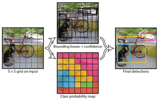
Figure 2. In the YOLO architecture, an input image is divided into an $S\times S$ grid where each grid cell predicts B bounding boxes defined by position, size and confidence. The class probability map decides the final label of a high-confidence bounding box. By Redmon et al. [24].

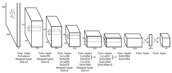
Figure 3. Basic network architecture of the YOLO framework. It has a Convolutional Neural Network (CNN) with over 20 connected layers. Source [24].

3. Approach

3.1. System Overview

The proposed system aims to provide a robust but versatile framework which is capable of classifying and counting vehicles passing by a stationary video camera. The systems design is based on special requirements like being able to operate on different kinds of roads and with a low recording frequency without any special configuration or user interaction. Especially the latter constraint is of special interest: Due to the ability of the system to work with remote video cameras such as Closed Circuit Televisions (CCTVs) restrictions in bandwidth are often the case. Consequently, such low frequencies make object tracking a challenging task considering solely raw video data. The classification and detection of vehicles is done with a pretrained state-of-the-art YOLO network. Furthermore, OpenCV (https://opencv.org) and cURL (https://curl.haxx.se) were used to perform common computer vision tasks and consume video streams respectively. The final component, the developed tracking and counting framework, then tackles the original goal of traffic monitoring.

3.2. Workflows

The system consists of two main processing workflows. The initialization phase shown in Figure 4a is comprised of two main processes: Detection and classification of objects as well as adaptation of the prediction model. The main goal of this phase is to gather information about the current traffic and road conditions. Depending on the view angle of the camera and the current traffic condition, the initialization phase needs more or less time to build up a sufficient model for later predictions. If the model has enough valid data the system changes over to the actual processing workflow. Moreover, sharing the first two components with the initialization workflow, the processing workflow consists of two additional components as depicted in Figure 4b: The tracking and counting parts. It is defined as an iterative process and analyzes frames as long as an input feed is available to finally count vehicles passing by the scene. The tracking component tries to find a set of detected objects in all the past frames and assigns random identifiers. Based on the identifier, already tracked and therefore unique vehicles are counted after leaving the scene.

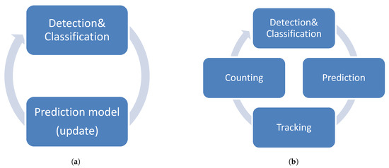
Figure 4. Model (a) shows the system loop for the initialization process. To guarantee the tracking and counting components to work properly the prediction model must be set up first. Model (b) shows the system loop for the actual counting framework consisting of four main components. Each processing unit delivers its data to the next one.

3.3. Core Components

3.3.1. Configuration and Input Feed

Before the system can perform in an applicable way several configurations have to be set up accordingly. Due to the high amount of different settings a configuration file was built up to maintain them easily at a single place. It is a simple JSON-file with a single (root) node. This file format was picked to be independent about the development platform, is easy to adapt and widely used. On start-up, the system tries to read and parse the configuration file and initializes itself. In Table 1, each of these settings are described in more detail and are subsequently used in order to create a configuration file in JSOn format. It mainly consists of values for the detection framework, which input feed is used and how the input feed should be processed. Furthermore, there are some more flags available to show additional information on the screen.

Table 1. Configuration file entries with additional information.

Key	Description	Value
namesFile	File location of the names file for each classifiable object type. Is needed for the detection framework while classifying.	String (absolute path to file)
configFile	File location of the configuration file needed for the detection framework for initialization.	String (absolute path to file)
weightsFile	File location of the weights file needed building up the detection framework neural network.	String (absolute path to file)
remote	Indicator if remote file location or local file location should be used.	Boolean (true/false)
videoFile	File location of a video file, e.g., mp4 file format.	String (absolute path to file)
remoteFile	Link to a remote file location that can be requested for a new frame.	String (web address)
requestInterval	Interval for requesting a new frame.	Integer (in milliseconds)
showHistory	Indicator if tracking history with additional object thumbnails should be shown or not.	Boolean (true/false)
manualMode	Indicator for disabling request interval and waiting for manual key input by the user to get the next frame.	Boolean (true/false)
showPrediction	Indicator for showing also predictions in a separate window.	Boolean (true/false)
detectionThreshold	Used to filter objects with confidence factors from classification. Objects with a confidence factor less than the detection threshold are not considered by the system for further processing.	Double (between 0 and 1)

As described in Table 1, the configuration file can be adapted for usage of local (offline) or remote (online) video sources. On the one hand, local video sources are just video files, e.g., in a mp4 file format, at a given path which are fed to the system. This fact makes debugging and offline testing of the system feasible. On the other hand, remote video sources are only web addresses. The system requests the site and tries to parse the image. This option is usually used for analysing live traffic on certain highways or roads for production usage. For both local and remote video sources the request interval behaves the same, hence restricts the system to only load new frames at a specified frequency.

3.3.2. Detection and Classification

Analysing incoming frames from video sequences, especially detecting and classifying multiple objects, is a complex task that needs advanced tools and methods to accomplish such a problem in an appropriate manner. Not only the issue itself, but also other requirements such as real-time or near real-time processing is often a crucial factor for a system to work properly or even work at all. The following text describes the detection and classification technique using the YOLO framework which is embedded in the proposed system.

As stated above, YOLO allows the system to detect and classify multiple objects within a single frame. Based on the trained data nearly every object type can be classified. Moreover, the classification itself it also provides a confidence factor for each type of object. This factor indicates how sure it is to be that kind of object. Furthermore, another benefit is the ability to provide the position of all the classified objects within the frame in the very same step.

In accordance to [24], many detection and classification systems refunction classifiers in order to implement the detection process. These systems take a classifier for an object and try to find them in various locations and scales in an image. An example of such a system uses deformable parts models (DPM) with a sliding window approach. There, the classifier runs at evenly spaced locations over the entire image. DPM uses a disjoint pipeline to extract static features, classify regions and predict bounding boxes for high scoring regions. The previously described method of incorporating Convolutional Neural networks (R-CNN) is also quite popular: After limiting the image to potential bounding boxes, selective search methods generate these bounding boxes while a CNN extracts features. Additionally, a SVM scores the boxes. Post-processing methods refine the bounding boxes and eliminate duplicate detections. Due to the number of different methods used each step has to be tuned independently. Also, the resulting system is very slow.

The utterly different approach which is implemented by YOLO is to reframe object detection by transforming the process of detection to a single regression problem. This way, both the bounding box estimation as well as the calculation of class probabilities are performed in a single step directly from the pixels of an image [24].

Moreover, as mentioned by Redmon [24] YOLO unifies the separate components into a single neural network. Thus, it can use features from the entire image to predict each bounding box. Therefore, all bounding boxes across all classes are predicted simultaneously which enables the network to reason globally about the full image as well as all the objects within the image.

Figure 2 shows an example about the process behind YOLO while analysing an image. First of all, YOLO divides the input image into a $S\times S$ grid of small cells. Each of these cells predicts B bounding boxes and confidence scores for those boxes. The score is a reflection of how confident the model is about a box including an object. Each bounding box therefore consists of 5 class probabilities C, which is the position of the bounding box $(x,y)$, the width and height of the box $(w,h)$ as well as the confidence factor c.

The design of the network is a typical Convolutional Neural Network (CNN) and was inspired by the GoogLeNet (https://ai.google/research/pubs/pub43022/) model for image classification as described in [24]. Furthermore, extracting features is done by the initial convolutional layers, whereas the fully connected layers are responsible for predicting output probabilities as well as the bounding box coordinates. Figure 3 shows the full network architecture of YOLO. It consists of 24 convolutional layers followed by 2 fully connected ones. At the end, there is simply a $1\times 1$ reduction layer followed by $3\times 3$ convolutional layers. The improved versions YOLOv2 and YOLOv3 have a slightly different network architecture in terms of the number of layers. The final output for the network is a $7\times 7\times 30$ tensor of predictions. It is encoded as a $S\times S\times (B\ast 5+C)$ vector with $S=7,B=2$ and $C=20$. This tensor was used for evaluating the first version of YOLO on the PASCAL VOC (http://host.robots.ox.ac.uk/pascal/VOC/) dataset.

An example of a prediction using the YOLO framework is shown in Figure 5. Corresponding to Redmon and Farhadi [26], due to its architecture YOLO tries to predict several different bounding boxes simultaneously where an object is suspected. Attached with multiple class probabilities for each type ranging from 0 to 1 this output can be filtered with a specified threshold. The final outputs are then bounding boxes with object class values over a specific threshold.

Figure 5. Prediction outputs from a single image by YOLO. Unfiltered output (a) showing all bounding box candidates where an object is suspected. (b) only shows predictions with values over a certain confidence factor. Labels representing object classes with the highest score. Source [23,24].

Conforming to [26], YOLOv3 is able to use multilabel classification on single bounding boxes. This is very useful when evaluating the framework with datasets including many overlapping labels, i.e., woman and person for the same object. Additionally, version 3 predicts boxes at several different scales and has also the ability to predict an increasing number of classes at once. Nonetheless, it comes with better performance regarding computation time due to slight changes in the network model as well as improvements in internal calculations. Figure 6 shows the performance of the YOLOv3 suite comparing to other frameworks. YOLO has a much better performance regarding computation time with nearly similar accuracy. YOLOv3 is about three times faster whereas past YOLO versions struggled with small objects. However, version 3 uses multi-scale predictions which produces better results regarding accuracy. The evaluation is based on the COCO dataset (http://cocodataset.org/) computed on a NVIDIA Titan X GPU.

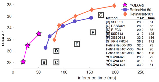
Figure 6. YOLOv3 significantly outperforms other detection methods with comparable accuracy in terms of computation time. Test results based on computations on a NVIDIA Titan X GPU evaluating images from the COCO dataset. Source [26].

Based on [24], YOLO has pretrained convolutional layers using the ImageNet 1000-class competition dataset (http://image-net.org/). The first 20 layers were pretrained with the underlying Darknet framework. The training was stopped after they reached about the same accuracy as the GoogLeNet models. The rest of the convolutional layers as well as the fully connected layers for detection are added with randomly initialized weights. Due to the base version of YOLO suffers from poor detection results for objects with varying sizes, where [25] proposed a multi-scale training as an improvement. Therefore, every few iterations the input image size changes. The model is now able to predict well across a variety of input dimensions. It can now detect predictions at different resolutions. Additionally, YOLO can also be trained with own datasets.

Stated by [23], YOLO is an open source object detector and classifier. The source code can be found on the official Github repository (https://github.com/pjreddie/darknet). Due to the fact that the original implementation is only testable and compilable on MacOS or Linux an additional repository (https://github.com/AlexeyAB/darknet) provides a Windows version. It is a fork from the original repository and is being maintained continuously.

As mentioned before, YOLO comes with pretrained convolutional weights what makes experimenting easier for the users. After installing the base system YOLO is ready to be applied instantly. All necessary files and information can be found on the official project website (https://pjreddie.com/darknet/yolo/). Furthermore, there are also versions with additional dependencies available, such as OpenCV and CUDA. According to [23], YOLO is about 500 times faster on GPUs with CUDA support in comparison to CPUs due to its ability to compute several tasks simultaneously. OpenCV is mainly used due to the extended support for image formats as well as viewing the results immediately without the need to store them on the disk first and open it separately.

YOLO comes with an own configuration file. It is used for initializing the CNN with basic settings at startup. Additionally, the file includes entries for test and training configurations as well as settings for all the different layers. Table 2 describes the most important settings in more detail.

Table 2. Most important YOLOv3 configuration file entry descriptions.

Key	Description	Value
batch	Also known as batch size. Indicates how many image samples are used before the network updates its weights during the training process. Is often used to save time when training with huge datasets.	Integer (multiples of 2)
subdivision	Lets you specify a subdivision of the batch size during training. This is helpful if you do not have enough memory to process all images at once. The system uses then batch/subdivision number of images.	Integer (multiples of 2)
width/height	Input image size. The image will be resized to $width\times height$ pixels before processing. In general, the higher the resolution the better the results. During training, higher values increase training time.	Integer (multiple of 32)
channels	Number of color channels while processing. For RGB images $channels=3$.	Integer
momentum	Penalizes large weight changes between iterations during training.	Double
decay	Penalizes large values of weights to prevent overfitting during training.	Double
learning_rate	Controls how fast the network learns.	Double
momentum	Penalizes large weight changes between iterations.	Double

3.3.3. Prediction Modelling

The proposed system operates with sequences from publicly and remotely accessible video cameras. Most of the time these public cameras are mounted above the roads, e.g., under bridges or special fixtures and record vehicles on roads with high traffic such as highways. Based on this fact, the following relevant assumptions can be made: (i) The analyzed sequences are mainly recorded on highways high above the street. The perspective of the camera is situated above the street with vehicles driving towards the camera, away from the camera or both. Additionally, there are seldomly significant bends on highways, hence the driving direction is very straight. (ii) On highways, the driving speed of all the vehicles passing by is quite similar. Thus, the covered distance between all the vehicles is nearly the same. However, this assumption is not valid for special cases such as congestions.

First of all, the prediction model saves all the positions from vehicle detections with additional data such as the frame count. If the model has enough data points from all the past frames it tries to form associations between these points. The goal of this task is to find possible driving paths in successive frames considering certain limitations: Data points are only valid if they come from successive frames to keep temporal ordering, lines between data points must stay inside a set range of angles to encourage rather straight driving paths and the distance between associated data points must be similar due to the assumed similar velocity of the vehicles.

Figure 7 shows a schematic illustration of the initialization process of the prediction model. It tries to find driving paths based on the gathered data points from the detection and classification component. This initialization phase is completed when a certain number of driving paths are available. However, it gets continuously updated in order to react to changing traffic parameters. The discovered driving paths are used later for estimating positions of vehicles in future frames.

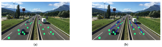
Figure 7. Schematic illustration of the prediction model setup. Detections (circles) from all the last frames are saved (a). The prediction model tries to associate these data points to get driving paths (lines) based on specific limitations (b). Source [27].

After completion of the initialization phase, the prediction model is able to estimate future positions of detected vehicles. As exemplified by Figure 8, the prediction model is asked to estimate positions of currently detected objects. Depending on the current positions of the detected vehicles, the prediction model picks the path which has a minimal distance for each of the detections. Each path is associated with an angle and a distance. This data is used to calculate a future position by simply adding the path such as a vector on top of the current position.

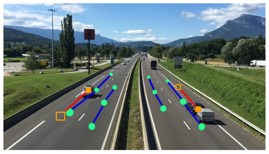
Figure 8. Exemplary prediction model visualization: The position of current detections (filled rectangles) are extended with data from the nearest driving paths (lines) to get future positions (framed rectangles). Screenshot taken from video (https://www.youtube.com/watch?v=nt3D26lrkho).

3.3.4. Tracking System

The tracking system receives the detections from a single frame enriched with the corresponding predictions for every detected object. For the used tracker the aforementioned information is necessary to accomplish tracing of objects under restricted circumstances which may occur in a usage scenario of the system. OpenCV comes with a huge variety of different tracking algorithms and frameworks. These methods are well tested and promising, but are usually only applicable for video streams with 25 or more frames per second. Depending on the speed of objects certain tracking algorithms work well down to about 7 FPS where the scene does not lag that much. Without any additional data, simple tracking frameworks fail completely in cases with low frame rates because object positions can change significantly from one frame to the next, especially when a high amount of objects is involved.

Based on these experiences solely raw video data will not achieve promising results for the mentioned issue. Additional information in the form of estimated object positions enable the tracking framework to compare just two object locations. Based on the assumption that the prediction model delivers accurate results, the estimated position from the last frame and the actual position from the current frame will overlap. In that case a simple distance tracker is a perfect fit because it only needs these two locations for a single object. Figure 9 is an example of such a distance tracker: If the additional estimated positions for every object are precise enough, the frequency of frames per second has only little effect on the tracking algorithm.

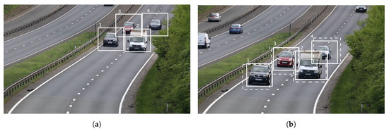
Figure 9. Tracking vehicles with predictions at low FPS. Each of the four objects gets detected in the first frame (a). The tracking algorithm tries to match objects based on a minimum distance to the predictions (dashed boxes) in the next frame (b). An association can be performed without the need for analysing the visual appearance of objects which can change greatly on low FPS. Source: Youtube.

3.3.5. Counting

As the name indicates this process is responsible for counting all objects passing by. Due to the fact that the proposed system should not only deliver proper results for a specific road scene, the counting mechanism should also be designed as abstract as possible. The counting process is the last part of the system loop and gets all necessary data from the preceding tracking framework. A list of all tracked objects enriched with additional information such as object ID, current position, object type and a list of frames is provided by the tracing process. The mentioned list of frames can be seen as a history of where and when the same object was detected and associated with the same identifier.

Counting is only performed with data received from the tracking process. If an object was tracked successfully several times it is considered to be positioned on a valid trace. Due to the nature of recording from static cameras objects enter and leave the scene regularly. At some point in time they cannot get tracked anymore because they get out of sight. This also means that the history of frames will not change anymore and that is the point where the counter can increase the number of encountered vehicles.

To not take any tracking errors into account the counting system filters the tracing history for valid objects. Such errors can occur due to partial or complete occlusion, e.g., on high traffic scenes, or when the detector itself delivers wrong detections. As a result, objects which are tracked only a small number of times are considered to be incorrect, hence will not be used by the counting framework at all.

The counting system delivers the total count of objects passing by. Furthermore, the counting process has access to additional information such as the object class. For this reason the system can also count not only the total number of objects, but also the number of objects per object class. See Figure 10b for a visual demonstration of the counting process.

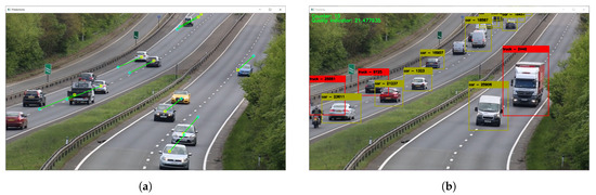
Figure 10. Demonstration of the tracking and counting phase. Based on the predictions from the prediction model (a), the tracking component can track objects successfully (b). Additionally, passed by objects are counted with help of the tracking results.

4. Evaluation and Limitations

There are three main aspects which are crucial for the proposed system: Generalization, classification and counting. First of all, the main goal of the system is to work under different traffic conditions without the need for manual user input or configuration changes. In other words, the system should be capable of abstracting well enough to also achieve proper performance in difficult conditions. Another requirement of the system concerns classification. The program should be be able to classify different vehicle types correctly. The most important vehicle types are trucks, cars and motorbikes. Last but not least, the traffic measurement consists of counting vehicles passing by.

4.1. Video Data

Due to the fact that the evaluation should be reproduceable with different settings for the same scenery, the video sequences are all available for free and were broadcasted on YouTube via the YouTube Live functionality. Three 1280 × 720 pixel scenes with 10 min duration and 30 frames per second were recorded with a free software tool for offline evaluation.

4.2. Counting Results

The following section evaluates three different traffic scenes. Each of them has a specific characteristic in order to get a broader sense of the proposed classification and counting system. The evaluation of the scenes is done with different request intervals, due to the fact that the performance of the system changes rapidly when operating under different settings. For each request interval there is a screenshot showing the prediction model as well as a table with the corresponding counting results. The prediction model shows the estimated driving paths during operation which are marked as coloured lines. Each of the resulting tables for every analysed request interval shows the actual vehicles on the scene, the counted objects by the program as well as the sum of them. Furthermore, each table is split up into the detected vehicle types. These tables are used to calculate the actual error rate of lost vehicles missed by the program or of additional vehicles detected by the system.

4.2.1. Traffic Approaching a Toll Station

One of the road parts analysed by the counting and classification application is a toll station in Russia. As expected the road characteristics are similar to most such stations around the world. There are three driving lanes at the bottom of the frame which splits up into eight lanes. Each of the eight lanes ends at a barrier where the cashier or a cash machine is located. The view angle of the camera is about 30° from the top to the ground. Furthermore, it is located at the right side of the lanes recording the traffic from the back, hence all vehicles are driving away from the camera. Additionally, the video camera records an area up to about 400 m to have a greater angle to record. However, this means that all vehicles are of little size.

For this scenario the evaluation is done with three different request intervals, namely 500 ms, 1000 ms and 1500 ms. For each of these request intervals, Figure 11 shows the corresponding prediction models with the estimated driving paths. In principle these driving paths are nearly the same for all the request intervals due to the wide area of recorded roads.

Figure 11. Prediction model visualizing the driving paths at a toll station. (a–c) have request intervals set at 500 ms, 1000 ms and 1500 ms, respectively.

However, the counting results differ greatly. Table 3 shows the outcome of the proposed application. The prediction model needs around 30 s to built itself up, the tracking and counting begins immediately afterwards. The results show that from the 111 vehicles only 7.2% are not counted successfully. After increasing the request interval to 1000 ms, the counting gets worse as depicted in Table 4. For this setting the prediction model needs about 1 min and 9 s for initialization. The amount of lost vehicles increases, the error rate is 21.9%. This is due to the detection issues of small vehicles. Objects driving away from the camera covering great distances with this setup, hence becoming smaller in size quicker. A continuous tracking is getting more difficult with increasing request interval. Same holds true for Table 5. Here the error rate is 43.2% with a request interval of 1500 ms.

Table 3. Counting results per vehicle type from a toll station with 500 ms request interval.

		Actual
		Truck	Car	Motorbike	Lost	Sum
Counted	Truck	0	0	0	0	0
	Car	1	102	0	0	103
	Motorbike	0	0	0	0	0
	Lost	0	8	0	0	8
	Sum	1	110	0	0	111

Table 4. Counting results per vehicle type from a toll station with 1000 ms request interval.

		Actual
		Truck	Car	Motorbike	Lost	Sum
Counted	Truck	0	0	0	0	0
	Car	1	63	0	0	64
	Motorbike	0	0	0	0	0
	Lost	0	18	0	0	18
	Sum	1	81	0	0	82

Table 5. Counting results per vehicle type from a toll station with 1500 ms request interval.

		Actual
		Truck	Car	Motorbike	Lost	Sum
Counted	Truck	0	0	0	0	0
	Car	1	41	0	0	42
	Motorbike	0	0	0	0	0
	Lost	0	32	0	0	32
	Sum	1	73	0	0	74

4.2.2. Traffic on a Bridge

In this section the counting and classification system analyses traffic on the Confederation Bridge in the East of Canada. Basically, the specifications of the recorded area are very simple: There are two driving directions, each of them with a single lane. The camera position is on top of the bridge recording traffic driving to and away from the camera. The road is in the middle of the scene. However, the scene itself mostly consists of the surrounding sea. The horizontal area of the bridge covered by the camera is great, hence cars can be seen from afar as little dots becoming bigger when approaching. The same holds true the other way around from the other driving direction.

As shown in Figure 12, the driving paths can be built up successfully for the relevant request intervals. The greater the interval is the bigger gets the covered distance from one frame to the other. Hence, the driving paths also increase in size.

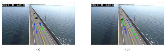
Figure 12. Prediction model visualizing the driving paths on the Confederation Bridge in Canada. (a,b) depict request intervals of 250 ms and 500 ms respectively.

Due to the fact that the detection and classification framework has its difficulties detecting small objects the biggest request interval possible is 500 ms. With intervals greater than that in combination with the high driving speed on the bridge it is not possible for the detection framework to detect the same object multiple times. This fact is also related to the big difficulties while counting. As depicted in Table 6 the error loss for a request interval of 500 ms is 67.1%. A successful counting of vehicles requires a proper tracking of those. However, the driving speed is too high to allow the framework to process them several times. Decreasing the request interval to 250 ms decreases the error rate to 51.1%. The corresponding counting values are shown in Table 7. The poor performance regarding the vehicle speed and view angle can be concluded by the initialization times of the prediction model. For 250 ms it is 59 s and 3 min 39 s for the request interval of 500 ms.

Table 6. Counting results per vehicle type from the confederation bridge with 500 ms request interval.

		Actual
		Truck	Car	Motorbike	Lost	Sum
Counted	Truck	19	0	0	0	19
	Car	0	9	0	0	22
	Motorbike	0	0	0	0	0
	Lost	5	47	5	0	57
	Sum	24	56	5	0	85

Table 7. Counting results per vehicle type from the confederation bridge with 250 ms request interval.

		Actual
		Truck	Car	Motorbike	Lost	Sum
Counted	Truck	35	10	0	0	45
	Car	0	22	0	0	22
	Motorbike	0	0	0	0	0
	Lost	0	61	9	0	70
	Sum	35	93	9	0	137

4.2.3. Traffic on A Highway

Another road type which is typically recorded is a highway. The classification and counting system analyses one in a province in the Netherlands called Gelderland. The road is recorded in a 45° angle from the side. The course of the road is a slight left curve and vehicles are entering and exiting the road on both ends. One end is on the bottom left of the image, the other one on the top right. Due to the slight curve vehicles at the top right end are recorded a long time which results in a lot of small vehicles in a restricted area. In the middle of the recorded road it splits itself up to an exit to the left. In total there are two lanes for each direction.

Figure 13 shows the driving paths generated by the prediction model for the corresponding request intervals, namely 500 ms, 1000 ms and 1500 ms. Noticeable is the distribution of the driving paths in regard to the request intervals. They are more focussed for lower intervals. This is due to the fact that the proposed system detects more vehicles in that restricted are on the top right where the vehicles are also more focussed. If the request interval is lower, the more detections the system performs. Hence, this also results in more updates for the prediction model and therefore more driving paths in that area.

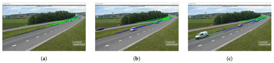
Figure 13. Prediction model visualizing the driving paths on a highway in the Netherlands. Request intervals are 500 ms in (a), 1000 ms in (b) and 1500 ms in (c).

As mentioned before a majority of driving paths are focussed on a small area on the top right for the recorded highway. This fact also reflects in all the counting results for the corresponding request intervals. The 500 ms results in Table 8 shows the greatest error. There is a total of 163 cars in the recorded sequence. However, the counting and classification framework counts another 172 cars in addition. In total this is an error rate of 86.4% for all the vehicles in terms of additional object counts. This is a result of the focussed driving paths. For the regions where no paths are constructed vehicles get counted as often as they are detected because they cannot be associated by the prediction model with other vehicles. Therefore, the lower the request interval, the more detections are performed, hence leading to an additional counting. The same holds true for the 1000 ms interval shown in Table 9. The error rate in terms of additional counting is 18.6%. This decreased number is because of the higher request interval where vehicles are not detected so often. For the interval with 1500 ms the results change. There are no more additional vehicles counted as depicted in Table 10. However, now the error is due to lost vehicles. In total the corresponding error rate is 24.5%. As a reason of the high traffic in the scene, the prediction model needs around 12 s for initialization for every request interval.

Table 8. Counting results per vehicle type from a highway with 500 ms request interval. Nearly every vehicle is counted twice.

		Actual
		Truck	Car	Motorbike	Lost	Sum
Counted	Truck	22	0	0	0	22
	Car	10	163 (+172)	0	0	173 (+172)
	Motorbike	0	0	0	0	0
	Lost	0	0	4	0	4
	Sum	32	163	4	0	199 (+172)

Table 9. Counting results per vehicle type from a highway with 1000 ms request interval. There are more vehicles counted then available.

		Actual
		Truck	Car	Motorbike	Lost	Sum
Counted	Truck	22	0	0	0	22
	Car	10	158 (+36)	0	0	168 (+36)
	Motorbike	0	0	0	0	0
	Lost	0	0	4	0	4
	Sum	32	158	4	0	194 (+36)

Table 10. Counting results per vehicle type from a highway with 1500 ms request interval.

		Actual
		Truck	Car	Motorbike	Lost	Sum
Counted	Truck	9	0	0	0	9
	Car	10	126	0	0	126
	Motorbike	0	0	0	0	0
	Lost	13	30	4	0	47
	Sum	32	156	4	0	192

4.3. Additional Limitations

Moreover, the detailed counting results there are several more restrictions while analysing traffic on video sequences. Some examples about additional limitations are depicted in Figure 14. First of all, different weather conditions can have a great effect on the overall performance of the system. Fog, rain or snow can change the recorded scenario completely. On the one hand, the detection framework cannot properly detect vehicles if they are not entirely visible anymore due to occlusion. Another factor are sudden reflections on the road itself because the surface gets wet and vehicles have to drive with lights on. On the other hand, not the road conditions itself, but also the camera parameters can change. Rain or snow can pollute the lens which obviously leads to a restricted performance of the overall system.

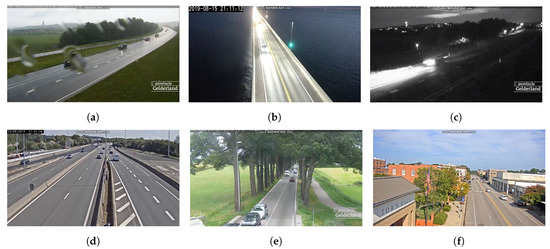
Figure 14. Known limitations in different environmental situations. Rainy conditions can smudge the camera (a). However, if there is not too much spray from the vehicles tracking is possible. Night situations with artificial light (b) or complete darkness (c) decrease the performance of the system rapidly. In some cases it is not even possible to detect a vehicle. Highways with multiple lanes and exits lead to difficulties estimating driving paths (d), rapid congestions, e.g., due to traffic lights impose complications in terms of tracking (e). Furthermore, parked vehicles in towns are also considered as active objects resulting in wrong driving paths (f).

Additionally, as a result that the system analyses real-world scenarios, the day-night rhythm has to be considered as well. In some cases artificial light brightens the scene too much, thus vehicles or vehicle types are not distinguishable anymore. For scenes with complete darkness the detection of vehicles is nearly impossible. Most of the time only the front or back lights of the vehicle are identifiable, even for the human eyes. Furthermore, if vehicles are driving towards the camera the scene gets masked completely because of the high beam of vehicles.

Another difficult scenario are multi-lane highways with exits or barriers. In principle, the prediction model needs constant traffic for all of the road parts in order to estimate the driving paths correctly. If the driving directions are separated and one of them is more used than the other tracking often leads to wrong results. This is a result of the wrong estimations of future positions from the prediction model.

In some cases traffic scenes are recorded just before traffic lights. This often leads to rapid congestions on the one end of the scene whereas on the other end there is a normal traffic flow. Therefore, the prediction model cannot update its internal state accordingly which leads to difficulties in tracking of the congested vehicles.

A special issue can be observed in town regions. There, traffic scenes do not show the roads itself, but also parked vehicles besides the road. Due to the fact that the prediction model tries to find driving paths based on the detections from all the previous frames such objects will also be considered. Hence, this results in wrong driving path estimations. At the end, a proper tracking and counting of vehicles cannot be guaranteed.

Due to the fact that the restricted bandwidth regarding remote camera accesses often results in a low image quality or resolution it can lead to problems detecting vehicles. The lower the resolution of the image the smaller the vehicles. The detection and classification framework has difficulties identifying such objects. For the reason that every other module relies on the initial detections low resolution or quality decreases the overall performance of the system.

5. Conclusions and Future Work

In this paper, an approach towards developing a general system for classification and counting of vehicles on ordinary webcam pictures is presented. Global traffic is steadily increasing which raises the need for intelligent traffic measurement systems. Due to the fact that modern computer systems can now process a large amount of data in real time there are new ways of developing surveillance applications. Furthermore, all-time connected devices such as camera systems on the road can deliver traffic scenes on the fly which can be processed automatically by autonomous systems.

As an alternative to induction loops a more generic and flexible approach for metering traffic is presented. Based on remote accessed cameras which deliver live-feeds from certain traffic hotspots a computer application analyses frame by frame. Therefore, the proposed system uses common computer vision and machine learning techniques in a hybrid application. The tracking and counting is of special interest due to the fact that the system operates in a restricted environment, e.g., processes video data with low frames per second.

The proposed application is built up using different, independent modules which all contribute to the overall classification and counting system. It is organized in a never ending system loop beginning with the gathering of data from an input feed reaching to the counting of vehicles based on their types.

One of the main modules is the detection and classification framework. Therefore, a state-of-the-art Convolutional Neural Network (CNN) is used. This framework is called YOLO which stands for “You Only Look Once” and is an open source implementation of the Darknet suite. Depending on the installed hardware YOLO is capable of classifying multiple objects within a single frame in real-time. Additionally, it can also deliver the exact position and size in the frame of all the detected objects in the very same step, hence it has to look on the image only once. YOLO is outstanding regarding object classification and detection in terms of computation time.

Another key component of the proposed system is the prediction model. The goal of this module is to estimate the next position of every object from the current frame to the following one. Prediction modelling for a tracking framework is not always necessary. However, the system has to face special requirements in real-world scenarios which have great effect on the tracking performance. Due to the fact that the system should work with different kinds of road types and traffic directions, predicting the next position limits the search space for tracking. Hence, it is often needed to find the same object in the following frames. Furthermore, video data from remote camera accesses are often restricted in bandwidth. This fact leads to quality issues regarding the image resolution, sharpness or reduced frames per second. For the latter objects passing by cover big distances between the separate frames which have great impacts on the tracking performance needed for counting. Basically, estimating the next position or state of an object adds additional information to the raw image data which helps the tracking software to improve its performance and stability. To overcome the mentioned problems the prediction model tries to estimate driving paths without the need for user interaction or specific settings.

Based on several assumptions the prediction model adapts to the different traffic scenes automatically. In the initial phase of the systems life-cycle the model initializes itself with the detections from the detection and classification component. The prediction model saves all the positions from the detections with additional data such as the frame count. If the model has enough data points from all the past frames it tries to make associations between these points. The aim of the prediction model is to find possible driving paths in successive frames.

The goal of the evaluation process is to find out how robust the used camera-based traffic measurement system under certain conditions is. There are three main aspects which are crucial for the proposed system: Generalization, classification and counting. The main goal of the system is to work under different traffic conditions without the need for manual user input or configuration changes. In other words, the system should be capable of abstracting well enough to achieve also proper performance in difficult conditions, e.g., high traffic scenes or on rainy days. Another requirement of the system is regarding the classification. The program should be capable of classifying different vehicle types correctly. The most important vehicle types are trucks, cars and motorbikes. Last but not least, the traffic measurement consists of counting vehicles passing by. If the counting is done right this information helps to provide estimations about the current traffic flow. These predictions can then be used for intelligent driving assistants, e.g., in navigation systems to bypass congestions on the road.

The evaluation is made on an ordinary computer system with a GPU supporting CUDA to enable real-time processing of video data. The data sources were available on the Youtube Live platform where several organizations were streaming traffic in real-time. To run the video sequence with different settings some passages of the videos were recorded. All video streams were analysed multiple times using different request intervals, hence simulating the restricted environment regarding the frequency of frames.

As a conclusion, the robustness of the proposed system under real-world scenarios could not be proven. For some restricted cases such as simple, mono-directional roads the error rate of lost vehicles can be held under 10%. There, the prediction model can estimate the driving paths correctly. For more difficult scenarios such as long distance roads or multi-lane highways with several exits the prediction model has its problems finding the right driving paths. For such cases the error rate is above 40%. In addition, the detection and classification framework has its flaws regarding different weather conditions such as rain, fog or darkness. Due to the fact that the prediction model only relies on the detection from the preceding module the overall performance decreases. Furthermore, if the traffic is not equally distributed between multiple driving directions the prediction model often estimates positions wrong because of no or less available driving paths. Depending on the request interval this leads to more or less additional counts of vehicles because the tracking is not possible anymore. Summarizing, the proposed system is capable of processing simple roads only, a generic approach is not found yet.

Outlook

To develop a more solid system which is able to deal with this versatile environment, several improvements need to be considered. This can be done as a future research to reach a more stable and less error-prone system. The following list describes suggested improvements related to discovered defects within this paper in more detail:

• Detection and classification
  First of all, the detection and classification framework has to improve its performance in regard to small sized vehicles. This can either be done by running the system with a better hardware (GPU) or by training the model specifically for small vehicles. Furthermore, training the framework with samples from different weather conditions may also have an positive effect of the detection and classification performance.
• Prediction model
  Estimating the driving paths only by the raw detections from the preceding frames leads to too many different possible tracks, hence resulting in wrong estimations and tracing of objects. Therefore, enriching these data with additional information helps to estimate the right driving paths. Another idea would be a post-processing step while updating the prediction model. A filter could remove wrongly detected paths with the help of the already established ones. Furthermore, added driving paths could be split up into different categories in regard to the driving direction. If the traffic is not equally distributed between the lanes it often leads to wrong estimations for the less frequent driving way because they are already outdated.
• Tracking
  Tracking of objects relies mostly on the detections and predictions from the previous modules. To improve the overall performance the tracking process could additionally consider other facts as well, e.g., driving direction, visual appearance or position on the screen. As a result the errors while matching cars from the different frames could be reduced.
• Counting
  The counting process of vehicles could be done not only based on vehicle types but also based on the driving direction. This is especially useful for highways to estimate possible congestions and the corresponding direction.

The proposed scheme has been developed within the context of a research project, which has ended shortly prior to the public release of the new YOLO version 4, which includes new additional methods which most probably lead to a further increase in classification, detection and counting rates. YOLOv4 uses the CSPDarknet53 as backbone network, which includes a spatial pyramid pooling block to increase the receptive field and separate out the most significant context features. A follow-up research project regarding not only the use of YOLOv4, but also a comparative study within the context of alternative frameworks such as those provided by Matlab, is planned for 2021.

References

- Pal, N.; Pal, S. A review on image segmentation techniques. Pattern Recognit. 1993, 26, 1277–1294. [Google Scholar] [CrossRef]
- Robert, H.; Linda, S. Image semgmentation techniques. Comput. Vis. Graph. Image Process. 1985, 29, 100–132. [Google Scholar]
- John, R. The Image Processing Handbook; CRC Press: Boca Raton, FL, USA, 2016. [Google Scholar]
- Sayanan, S.; Trivedi, M.M. Looking at Vehicles on the Road: A Survey of Vision-Based Vehicle Detection, Tracking and Behavior Analysis. IEEE Trans. Intell. Transp. Syst. 2013, 14, 1773–1795. [Google Scholar]
- Chang, P.; Hirvonen, D.; Camus, T.; Southall, B. Stereo-Based Object Detection, Classification and Quantitative Evaluation with Automotive Applications. In Proceedings of the IEEE Computer Society Conference on Computer Vision and Pattern Recognition, San Diego, CA, USA, 20–25 June 2005. [Google Scholar]
- Kenneth, D.-H. A Practical Introduction to Computer Vision with OpenCV; John Wiley & Sons: New York, NY, USA, 2014. [Google Scholar]
- Hankyu, M.; Rama, C.; Azriel, R. Optimal edge-based shape detection. IEEE Trans. Image Process. 2002, 11, 1209–1227. [Google Scholar]
- Wen, W.; Xiling, C.; Jie, Y. Incremental detection of text on road signs from video with application to a driving assistant system. In Proceedings of the 12th annual ACM International Conference on Multimedia, New York, NY, USA, 10–15 October 2004. [Google Scholar]
- Brutzer, S.; Höferlin, B.; Heidemann, G. Evaluation of background subtraction techniques for video surveillance. In Proceedings of the IEEE Conference on Computer Vision and Pattern Recognition (CVPR), Colorado Springs, CO, USA, 20–25 June 2011. [Google Scholar]
- Benezeth, Y.; Jodoin, P.; Emile, B.; Laurent, H.; Rosenberger, C. Comparative study of background subtraction algorithms. J. Electron. Imaging 2010, 19, 033003. [Google Scholar]
- Gary, B.; Adrian, K. Learning OpenCV: Computer Vision with the OpenCV Library; O’Reilly Media Inc.: Sebastopol, CA, USA, 2008. [Google Scholar]
- Adrian, K.; Bradski, G. Learning OpenCV 3: Computer Vision in C++ with the OpenCV Library; O’Reilly Media Inc.: Sebastopol, CA, USA, 2016. [Google Scholar]
- David, L. Object recognition from local scale-invariant features. In Proceedings of the 7th IEEE International Conference on Computer Vision, Kerkyra, Greece, 20–27 September 1999. [Google Scholar]
- Roberto, B. Template Matching Techniques in Computer Vision: Theory and Practice; John Wiley & Sons: New York, NY, USA, 2009. [Google Scholar]
- Jolly, M.-P.D.; Lakshmanan, S.; Jain, A.K. Vehicle segmentation and classification using deformable templates. IEEE Trans. Pattern Anal. Mach. Intell. 1996, 18, 293–308. [Google Scholar] [CrossRef]
- Serkan, O.; Ergun, E. Automatic vehicle identification by plate recognition. World Acad. Sci. Eng. Technol. 2005, 9, 222–225. [Google Scholar]
- Anil, J.; Robert, D.; Jianchang, M. Statistical pattern recognition: A review. IEEE Trans. Pattern Anal. Mach. Intell. 2000, 22, 4–37. [Google Scholar]
- Alper, Y.; Javed, O.; Shah, M. Object tracking: A survey. ACM Comput. Surv. 2006, 38, 13. [Google Scholar]
- David, L.; Lookingbill, A.; Thrun, S. Adaptive Road Following Using Self-Supervised Learning and Reverse Optical Flow. In Proceedings of the Robotics: Science and Systems, Cambridge, MA, USA, 8–11 June 2005. [Google Scholar]
- Ashit, T.; Matthies, L. Real-Time Detection of Moving Objects from Moving Vehicles Using Dense Stereo and Optical Flow. In Proceedings of the 2004 IEEE/RSJ International Conference on Intelligent Robots and Systems (IROS)(IEEE Cat. No. 04CH37566), Sendai, Japan, 28 September–2 October 2004. [Google Scholar]
- Benjamin, C.; Coifman, B.; Beymer, D.; McLauchlan, P.; Malik, J. A real-time computer vision system for vehicle tracking and traffic surveillance. Transp. Res. Part C Emerg. Technol. 1998, 6, 271–288. [Google Scholar]
- Harini, V.; Masoud, O.; Papanikolopoulos, N.P. Computer vision algorithms for intersection monitoring. IEEE Trans. Intell. Transp. Syst. 2003, 4, 78–89. [Google Scholar]
- Redmon, J. Darknet: Open Source Neural Networks in C. Available online: http://pjreddie.com/darknet/ (accessed on 8 July 2020).
- Redmon, J.; Divvala, S.; Girshick, R.; Farhadi, A. You only look once: Unified, real-time object detection. In Proceedings of the IEEE Conference on Computer Vision and Pattern Recognition, Las Vegas, NV, USA, 27–30 June 2016. [Google Scholar]
- Joseph, R.; Farhadi, A. YOLO9000: Better, faster, stronger. In Proceedings of the IEEE Conference on Computer Vision and Pattern Recognition, Honolulu, HI, USA, 21–26 July 2017. [Google Scholar]
- Joseph, R.; Farhadi, A. Yolov3: An incremental improvement. arXiv 2018, arXiv:1804.02767. [Google Scholar]
- Kiraly, V. Relaxing Highway Traffic. 2017. Available online: https://youtu.be/nt3D26lrkho (accessed on 8 September 2020).
© 2020 by the authors. Licensee MDPI, Basel, Switzerland. This article is an open access article distributed under the terms and conditions of the Creative Commons Attribution (CC BY) license (http://creativecommons.org/licenses/by/4.0/).