Learning Class-Specific Features with Class Regularization for Videos

Abstract

One of the main principles of Deep Convolutional Neural Networks (CNNs) is the extraction of useful features through a hierarchy of kernels operations. The kernels are not explicitly tailored to address specific target classes but are rather optimized as general feature extractors. Distinction between classes is typically left until the very last fully-connected layers. Consequently, variances between classes that are relatively similar are treated the same way as variations between classes that exhibit great dissimilarities. In order to directly address this problem, we introduce Class Regularization, a novel method that can regularize feature map activations based on the classes of the examples used. Essentially, we amplify or suppress activations based on an educated guess of the given class. We can apply this step to each minibatch of activation maps, at different depths in the network. We demonstrate that this improves feature search during training, leading to systematic improvement gains on the Kinetics, UCF-101, and HMDB-51 datasets. Moreover, Class Regularization establishes an explicit correlation between features and class, which makes it a perfect tool to visualize class-specific features at various network depths.

1. Introduction

Video-based action recognition has seen tremendous progress since the introduction of Convolutional Neural Networks (CNNs) [1,2]. The hierarchical application of 3D convolutional operations has been shown to effectively capture descriptive spatiotemporal features.

CNNs include multiple layers that are stacked in a single, hierarchical architecture. Features are calculated by successive convolutions. Kernels in early layers focus on simple textures and patterns, while deeper layers focus on more complex parts of objects or scenes. As these features become more dependent on the different weighting of neural connections in previous layers, only a portion of them becomes descriptive for a specific class [3,4]. Yet, all kernels are learned in a class-agnostic way. Consequently, much of the discriminative nature of CNNs is achieved only in the very last fully-connected layers. This hinders easy interpretation of the part of the network that is informative for a specific class.

We aim at forcing the network to propagate class-specific activations throughout the network. We propose a method named Class Regularization that relates class information to extracted features of network blocks. This information is added back to the network by amplifying and suppressing activation values with respect to predicted classes. Class Regularization has a beneficial effect on the nonlinearities of the network by modulating the effects of the activations. Owing to this, the architecture can effectively distinguish between the most class-informative kernels in each part of the network given a selected class. This procedure reduces the dependency on many uncorrelated features in the last fully-connected layers that are responsible for the final class predictions, essentially penalizing overfitting.

Our contributions are the following:

• We propose Class Regularization, a regularization method applied in spatiotemporal CNNs. The method does not change the overall structure of the architecture, but can be used as an additional step after each operation or block.
• We demonstrate that the relationships between classes and features can be visualized by propagating class-based feature information through normalized neural weights for each of the model’s building blocks.
• We report performance gains for benchmark action recognition datasets Kinetics, UCF-101, and HMDB-51 by including Class Regularization in convolution blocks.

We discuss advances in vision-based action recognition in Section 2. A detailed overview of Class Regularization appears in Section 3. Experiments are presented in Section 4. We conclude in Section 5.

2. Related Work

Significant advancements have been made in the recognition of actions in videos with the introduction of deep neural approaches that are based on the hierarchical discovery of informative features [5,6]. These architectures provide the basis to further accommodate temporal information.

Due to the indirect relationship between temporal and spatial information, one of the first attempts on video recognition with neural models was the use of Two-stream networks [7]. These networks contain two separate models that use still video frames and optical flow as inputs. Class predictions are made after combining the extracted features of the separate networks. Two-stream networks were also used as a base method for works such as Temporal Segment Networks (TSN, [8]) which use scattered snippets from the video and fuse their predictions. This approach sparked research on the selection of informative frames [9,10]. Other extensions of Two-stream networks include the use of residual connections [11,12] that share spatiotemporal information across multiple layers.

An alternative approach to capture temporal information in CNNs is through 3D convolutions [13]. 3D convolutions include an additional time dimension to the two spatial dimensions. 3D convolutions have been shown to outperform standard image-based networks [14] in video classification. A fusion of Two-stream networks and 3D convolutions has been explored with the I3D architecture [15]. The two spatiotemporal models are trained in parallel on frame and optical flow data, with the benefit of also processing temporal-only information. Further structures that have been explored with 3D convolutions include Residual Networks [16].

Inspired by depthwise and pointwise convolutions performed over image channels [17], researchers have introduced ways of splitting the 3D convolutions in subsequent 2D convolution operations. This can be achieved through either using spatial filters followed by temporal-only filters [18,19] or convolutions in groups [20,21]. Alternative implementations include the use of long-sequence and short-sequence kernels [22] and dimension-based iterations of time-width and time-height [23,24]. Others have worked on the minimization of the computational requirements by shifting activations along time [25]. Previous works that have touched upon regularization were aimed more at the overall temporal consistency of features (e.g., [26]) without the consideration of feature combinations that are most informative for some classes.

Although these techniques have shown great promise in terms of accuracy and computational performance, there is still a lack of better spatiotemporal representations for intermediate network layers. Currently, there is no standardized way of processing the temporal information. Our proposed method, named Class Regularization, fills this void as it can be added to virtually all network architectures with minimum additional computational cost in order to enhance the correlation between specific spatiotemporal features and the action class.

3. Regularization for Convolutional Blocks

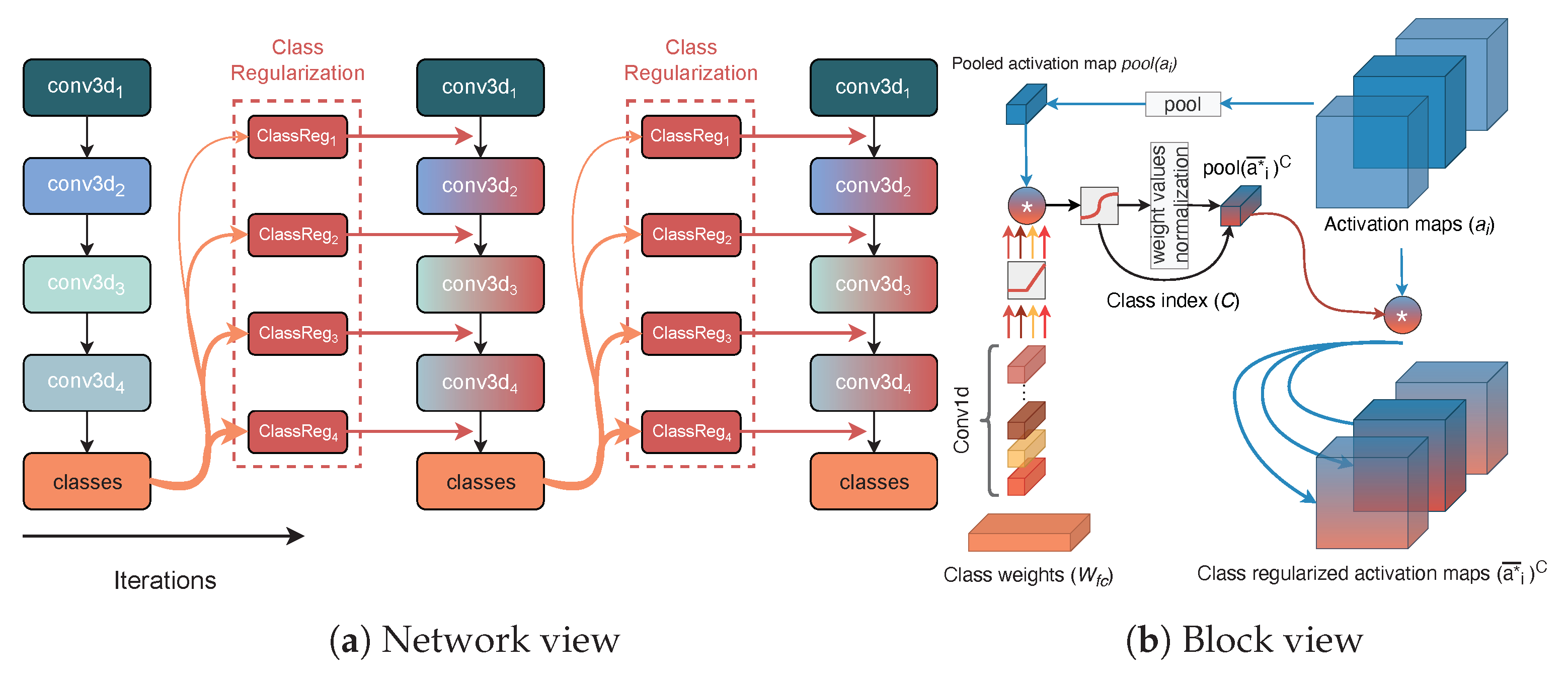
In CNNs, explicitly adding class information through regularization is challenging, given the increasing level of ambiguity of the model’s inner workings with respect to the network depth. We make the assumption that, when testing a video in a trained CNN, a speculative guess can be made on which class is represented by observing the activations produced at a certain layer. The underlying idea is that different kernels focus on different spatiotemporal patterns that appear in different classes. These guesses depend on the layer depth. Deeper network layers can distinguish class-specific features better because of the larger feature complexity. Therefore, guesses at different parts of the model should have consequently greater or lesser effect. To include the layer feature complexity, we define an affection rate ($\mathfrak{A}$) that specifies how the class predictions affect the network’s activation maps. The values are chosen given the layer depth and the level of uncertainty of their class estimates. The discovery of feature correspondence between the layer’s feature space and the class’s feature space is implemented through pointwise convolutions and by incorporating their kernel updates as part of the training procedure. A complete workflow of the regularization method appears in Figure 1.

3.1. Layer Fusion with Class Predictions

We first discuss the main process for finding class estimates based on extracted features from the convolutional block at depth i in the network. We start by creating a vector representation of the features as distributed between the activation’s channels for a spatiotemporal activation map input of size ($FxHxW$). Considering the produced activation map of the $i\mathrm{th}$ block (denoted as $a_i$), a global feature representation of the activations is created through a spatiotemporal sampling operation: $pool\left(a_i\right)$ (Equation (1)). The produced volume can be interpreted as a single vector descriptor containing a combination of the feature intensity values in the form of their average activations in a significantly lower dimensional space.

$$pool\left(a_i\right)=\frac{1}{F\times H\times W}\sum _{f=1}^F\sum _{h=1}^H\sum _{w=1}^W{a}_{(f,h,w,i)}.$$

(1)

To include class-based information in intermediate feature layers, we use the weights of the network’s final prediction layer $W_{fc}$. This allows to establish a relationship between previous and current iterations in a recurrent fashion, by taking class-specific features into account. To obtain feature alignment given the channel sizes for the current activation and the prediction weights, a one-dimensional convolutional operation ($conv=W_{fc}\ast \mathcal{W}$) is applied to the class weights with a kernel ($\mathcal{W}$) size of 1 followed by a $relu$ activation function.

Next, we use a standard matrix-to-matrix multiplication to create an association between the channel descriptor and each of the classes. The volume $Z_i$ is of size $\{Z_i^{\left[1\right]},...,Z_i^{\left[CL\right]}\}$, for $CL$ classes, with each unit $Z_i^{\left[j\right]}$ having the same channel dimensionality as $a_i$. This operation allows an early estimate for the indexes of the most relevant features for each class.

One could use the outputs of the multiplication as a separate loss function but we have two main reasons for refraining from doing so. First, due to the limited feature complexity, it is significantly more difficult to make educated class predictions in early layers of the network. This also corresponds to the notion of hierarchical feature extraction in CNNs. Second, through these multiple output points, multiple error derivatives are to be calculated which will slow down the training process significantly.

3.2. Fusion of Class Weight Vector and Spatiotemporal Activation Maps

Our aim is to let the produced class-based activations $Z_i$ become indicators for the most informative class features. With this, we aim at obtaining the maximum class probability through a standard softmax activation function applied on the activations. This converts the weighed sum logit score to a probabilistic distribution over all classes: $S\left(Z_i\right)$. Based on (5) in Algorithm 1, the index of the maximum class activation is selected (C) to define the class weight vector with the highest correspondence based on the class features of the layer.

Algorithm 1 Class regularization overview
1: Inputs:
Values of activation map $a_i$ for $i\mathrm{th}$ layer.
2: Outputs:
Class-regularized activations ${\left(\overline{a_i^{*}}\right)}^C$
3: $W_i\leftarrow relu(W_{fc}\ast \mathcal{W})$
	▹ Weight dimensionality conversion
4: $Z_i\leftarrow W_i\ast pool\left(a_i\right)$
	▹ Weighted sum per class neuron
5: $C\leftarrow \underset{j}{argmax}\{S\left(Z_i^{\left[1\right]}\right),\dots ,S\left(Z_i^{\left[CL\right]}\right)\} \forall S\left(Z_i^{\left[j\right]}\right)=\frac{{ϵ}^{Z_i^{\left[j\right]}}}{{\displaystyle \sum _{c\in 1,\dots ,CL}}{ϵ}^{Z_i^{\left[c\right]}}}$
	▹ Largest softmax activation class search
6: ${\widehat{W}}_i\leftarrow \mathfrak{A}\ast \frac{(W_i-min\left\{W_i\right\})\ast (1-\mathfrak{A})}{max\left\{W_i\right\}-min\left\{W_i\right\}}$
	▹ Weight scaling
7: ${\left(\overline{a_i^{*}}\right)}^C\leftarrow {\widehat{W}}_i^{\left[c\right]}\ast a_i$
	▹ Final weight regularization.

As we want to amplify activation features, we need to normalize weight vector $W_i$ before fusing it with the layer’s activation maps. Layer features that are less informative for a specific class should be scaled down, while informative ones should be scaled up. To this end, we set a value ($\mathfrak{A}$) which will be referred to as the affection rate. It determines the bounds that the weight vector will be normalized to (${\widehat{W}}_i$)—see step (6) in Algorithm 1. We are not using a standardization method as in batch normalization [27] that guarantees a zero-mean output. This is because we use a multiplication operation for including the class weight information to the activation maps. Therefore, zero-mean normalization will remove part of the information because values below one will decrease in the feature intensity. It also hinders performance as it effectively contributes to the occurrence of vanishing gradients because the produced activation map values would be reduced at each iteration.

In our final step, we inflate the normalized weight vector ${\widehat{W}}^{\left[c\right]}$ to match the dimensions of the spatiotemporal activation maps. We then perform a matrix-to-matrix multiplication between the activation maps of the layer $a_i$ and the normalized weights with the axis of symmetry being the depth or channel’s dimension.

3.3. Performing Updates to Regularized Volumes

Class Regularization is performed on activation maps in the network to manipulate the activation values of the upcoming operations. We underline that the value of the affection rate $\mathfrak{A}$ used in the normalization can be trained through a separate objective function. In addition, our method is independent of the training iteration or layer number that it is applied to, and can process examples independently for online learning. Therefore, the discovery of class connections can also be performed in minibatches, to then return regularized volumes over single or multiple class weights.

The feature representation that is captured ${\left(\overline{a_i^{*}}\right)}^C$ depends on the specific example $a_i$, the layer or block i of the architecture that the regularization was applied to, the chosen class C that was selected, and the affection rate $\mathfrak{A}$. The distribution inside ${\widehat{W}}_i^{\left[C\right]}$ has an expected value of 1 and a distribution of $2(1-\alpha )$. Due to the low computational overhead to back-propagate through the proposed method, the computation times are not significantly affected by including Class Regularization in a network.

3.4. Class Regularization for Visualizations

As Class Regularization is based on the injection of class-based information inside the feature-extraction process, a direct correlation between classes and features is made at each block in which the method is applied. Being able to represent the class features given a different feature space improves the overall explainability capabilities of the model. Through feature correlation, the method alleviates the curse of dimensionality problem of previous visualization methods that rely on back-propagating from the predictions to a particular layer [28]. Since the classes are represented in the same feature space as the activation maps of the block, we can discover regions in space and time that are informative over multiple network layers. To the best of our knowledge, this is the first method to visualize spatiotemporal class-specific features at each layer of the network.

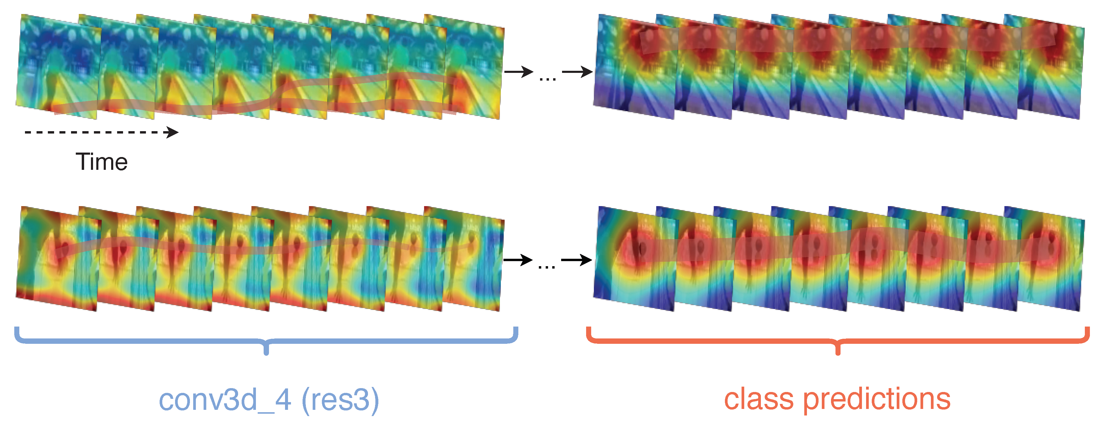
By extending the proposed algorithm to include an adaptation of Saliency Tubes [29] in each block, we can create visual representations of the features with the highest activations per class. We create two visual examples of the class bowling in Kinetics-400 to demonstrate class activations in different layers of the network (Figure 2). As observed in the clip segment, in both cases, early layer features are significantly less deterministic of the class and mostly target the distinction between foreground and background. In later layers, the focus shifts from the actor to the background in the predictions layer of the first clip. Ball and bowling pins are present at a wallpaper, which demonstrates that a strong still-frame visual signal is favored in case the action or objects within the action are occluded. In the second clip, the main field of focus of the network in the final layers is towards the area between the actor’s hand and the ball. We note that, by design, all network architectures used fuse all temporal activations to a single frame at their final convolution block, which only allows the visualization of spatial extension of the activations.

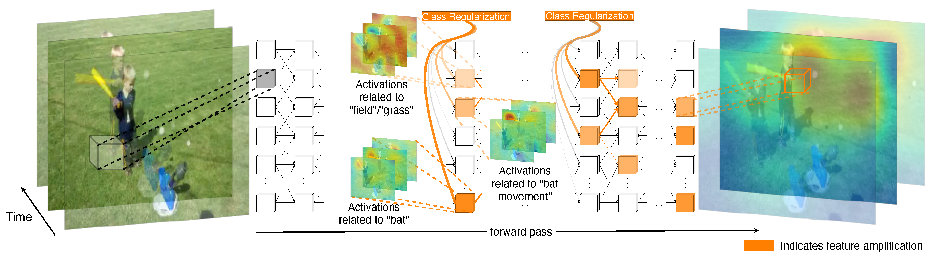
The amplification of layer features can also be visualized as in Figure 3. The top-3 kernels to be amplified for a baseball hit example correspond to spatiotemporal features such as the appearance of the bat, the field, and the movement of the bat during a swing. In addition, these amplifications are also propagated to deeper layers in the network through the connections of the most informative kernels.

4. Experiments

We demonstrate the merits of Class Regularization on the action recognition classification performance on three benchmark datasets, and using a number of widely used CNN architectures. Results are summarized in

Table 1. Architectures of 3D convolution models with and without class regularization. We note that in the Class Regularized networks, only an eighth of the additional parameters are trainable, with the rest corresponding to nontrainable class weights tensor duplicates.

Layer Name	3D ResNet101 (w/o CN)	3D Wide ResNet 50 (w/o CN)	I3D (w/o CN)
$con3d_1$	$7\times 7\times 7,64$ conv
$con3d_2$	$\left[\begin{array}{c}1\times 1\times 1\\ 3\times 3\times 3\\ 1\times 1\times 1\end{array}\right](\times 64)\times 3$	$\left[\begin{array}{c}1\times 1\times 1\\ 3\times 3\times 3\\ 1\times 1\times 1\end{array}\right](\times 128)\times 3$	$\left[\begin{array}{cccc}1\times 1\times 1& 1\times 1\times 1& 1\times 1\times 1& 3\times 3\times 3,\left(pool\right)\\ & 3\times 3\times 3& 3\times 3\times 3& 1\times 1\times 1\end{array}\right](\times 480)\times 2$
$ClassRe{g}_1$	- / $\alpha =0.9$	- / $\alpha =0.9$	- / $\alpha =0.8$
$con3d_2$	$\left[\begin{array}{c}1\times 1\times 1\\ 3\times 3\times 3\\ 1\times 1\times 1\end{array}\right](\times 128)\times 4$	$\left[\begin{array}{c}1\times 1\times 1\\ 3\times 3\times 3\\ 1\times 1\times 1\end{array}\right](\times 256)\times 4$	$\left[\begin{array}{cccc}1\times 1\times 1& 1\times 1\times 1& 1\times 1\times 1& 3\times 3\times 3,\left(pool\right)\\ & 3\times 3\times 3& 3\times 3\times 3& 1\times 1\times 1\end{array}\right](\times 832)\times 5$
$ClassRe{g}_2$	- / $\alpha =0.8$	- / $\alpha =0.8$	- / $\alpha =0.7$
$con3d_2$	$\left[\begin{array}{c}1\times 1\times 1\\ 3\times 3\times 3\\ 1\times 1\times 1\end{array}\right](\times 256)\times 23$	$\left[\begin{array}{c}1\times 1\times 1\\ 3\times 3\times 3\\ 1\times 1\times 1\end{array}\right](\times 512)\times 6$	$\left[\begin{array}{cccc}1\times 1\times 1& 1\times 1\times 1& 1\times 1\times 1& 3\times 3\times 3,\left(pool\right)\\ & 3\times 3\times 3& 3\times 3\times 3& 1\times 1\times 1\end{array}\right](\times 1024)\times 2$
$ClassRe{g}_3$	- / $\alpha =0.7$	- / $\alpha =0.7$	- / $\alpha =0.6$
$con3d_2$	$\left[\begin{array}{c}1\times 1\times 1\\ 3\times 3\times 3\\ 1\times 1\times 1\end{array}\right](\times 512)\times 3$	$\left[\begin{array}{c}1\times 1\times 1\\ 3\times 3\times 3\\ 1\times 1\times 1\end{array}\right](\times 1024)\times 3$	-
$ClassRe{g}_4$	(-) / $\alpha =0.6$	- / $\alpha =0.6$	-
predictions	global average pool, softmax unit group

. We further statistically compare the classification performance between predictions from different architectures and from different blocks within the same architecture.

For our experiments, we consider the widely used Kinetics-400 [30] dataset as a baseline. Then, each of the selected models is further fine-tuned on both UCF-101 [31] and HMDB-51 [32] by training the 1D convolutions inside Class Regularization to ensure a dimensionality correspondence between the new class weight vectors and the activation maps of each layer that the method is applied to. We further allow updates on the final two convolution blocks of the selected networks.

Training. The models trained on Kinetics are initialized with a standard Kaiming initialization [33] without inflating the 3D weights. This allows for a direct comparison between architectures with and without Class Regularization and to compare the respective accuracy rates. For all the experiments, we use an SGD optimizer with 0.9 momentum. Class Regularization is added at the end of each bottleneck block in the ResNets and at the end of each mixed block in I3D.

We use transformations for both spatial and temporal dimensions. In the temporal dimension, we use clips of 16 frames that are randomly extracted from different subsequences of the video. For the validation sets, we only use the center 16 frames. Spatially, we use a cropping size of $112\times 112$ and $256\times 256$ for fine-tuning. All models are trained for 170 epochs, as no further improvements were observed afterwards in our initial experiments with all three networks on Kinetics. We also used a step-based learning rate reduction of 10% every 50 epochs.

Datasets. Kinetics-400 consists of roughly 240 K training videos and 20 k validation videos of 400 different human actions. We report the top-1 accuracy alongside the computational cost (FLOPs) for each of the networks using spatiotemporally cropped clips. UCF-101 and HMDB-51 have 13 k and 9 k videos, respectively. They are used to demonstrate the transfer abilities of the proposed Class Regularization as well as the usability of our method in smaller datasets.

4.1. Main Results

A comparison between results of models trained from scratch on Kinectics-400 appears in

Table 2. Accuracy rates of different spatiotemporal convolutional architectures on the Kinetics-400 dataset.

Model	Backbone	Depth	# Params (M)	GFLOPS	Top-1 (%)
ResNet50-3D [16]	ResNet	50	36.72	80.32	0.636
ResNet101-3D [16]	ResNet	101	69.06	110.98	0.652
ResNeXt101-3D [16]	ResNet	101	69.06	148.91	0.667
Wide ResNet50-3D [16]	ResNet	50	140.94	72.32	0.640
I3D [15]	Inception	48	12.07	55.79	0.664
R(2+1)D-ResNet50 [19]	Resnet	50	34.86	89.14	0.645
R(2+1)D-ResNet101 [19]	ResNet	101	67.22	159.21	0.668
MF-Net [36]	ResNet	50	8.03	22.7	0.653
ResNet101-3D w/Class Regularization	ResNet	101 + 4	37.10	126.13	0.677
Wide ResNet50-3D w/Class Regularization	ResNet	50 + 4	141.32	82.67	0.653
I3D w/Class Regularization	Inception	48 + 3	69.44	62.96	0.678

. Existing networks consider a complete change in the overall architecture or convolution operations in models, which is computationally challenging given the large memory requirements of spatiotemporal models. New models need to be trained for a significant number of iterations in order to achieve mild improvements, while additionally using large datasets [34,35] for pretraining. In contrast, the proposed Class Regularization method is used on top of existing architectures and only requires fine-tuning the dimensionality correspondence between the number of features in a specific layer and the features that are used for class predictions. Overall, the largest improvements were observed on networks with larger number of layers, such as ResNet101-3D, in comparison to networks with lower number of layers, with the best performing architectures being I3D and ResNet101-3D with Class Regularization with 67.8% top-1 accuracy and 67.7% top-1 accuracy, respectively.

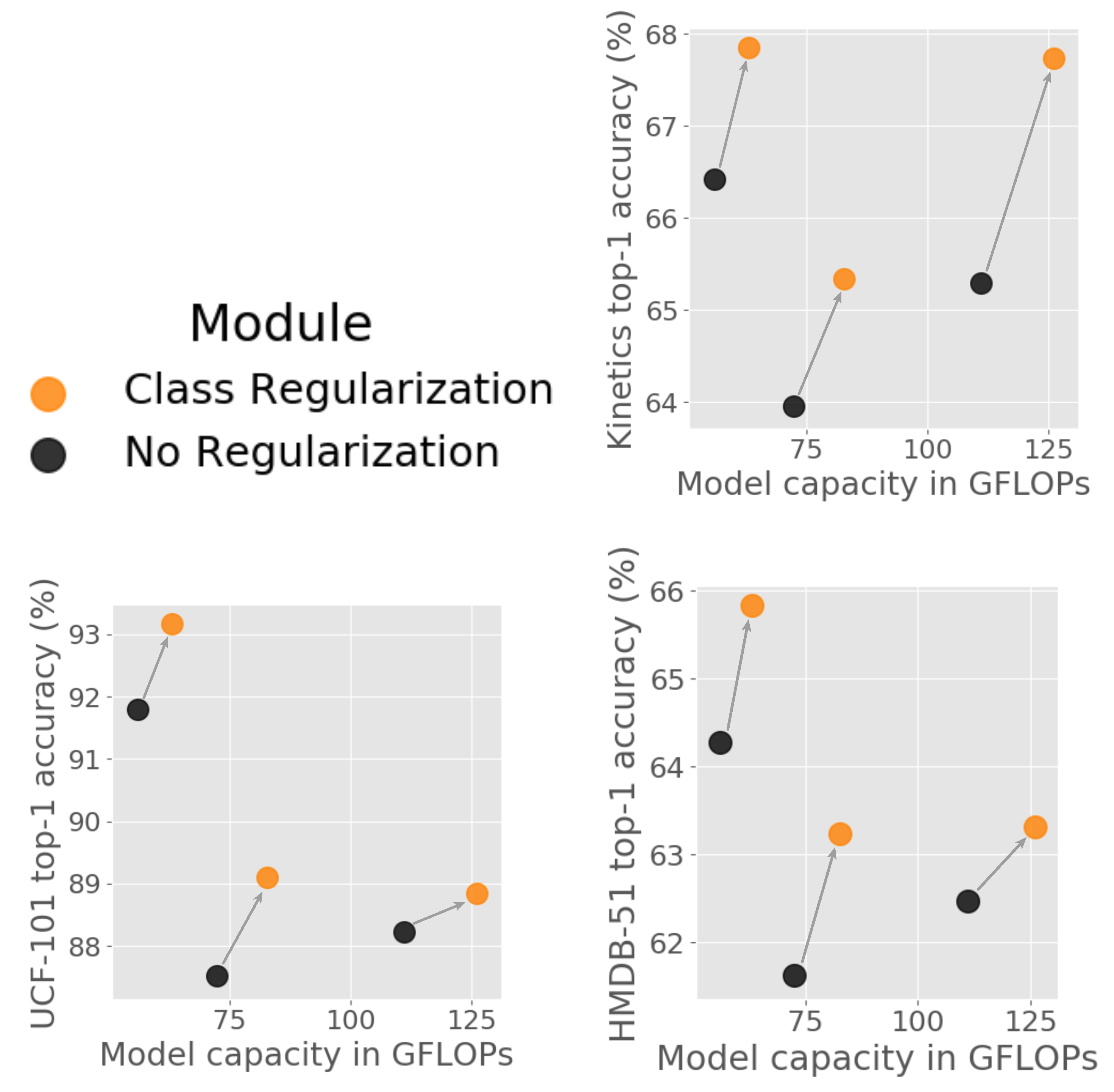
4.2. Direct Comparisons with and without Class Regularization

In

Table 3. Direct comparison of architectures with (in orange) and without (in black) Class Regularization blocks. Latency in msec.

Model	Added Latency	Kinetics	UCF101	HMDB51
ResNet101	-	65.29%	88.23%	62.47%
ResNet101	+ 98.786	67.74%	88.84%	63.31%
Wide ResNet50	-	63.96%	87.52%	61.62%
Wide ResNet50	+102.995	65.33%	89.11%	63.24%
I3D	-	66.42%	91.80%	64.27%
I3D	+68.34	67.85%	93.17%	65.83%

, we pairwise compare three architectures after training directly on Kinetics, and after adding Class Regularization blocks and fine-tuning. For each architecture and dataset, networks with Class Regularization outperform those without. The largest gain is observed in the 101-layer 3D Resnet (+2.45%), while we obtained improvements of +1.37% and +1.43% on the Wide-ResNet50 and I3D, respectively. Our approach appears to be especially useful for deeper networks. Since the effective description of classes is achieved through large feature spaces, Class Regularization significantly benefits models that include complex and large class weight spaces. The set of influential class features can be better distinguished with minimal computational costs, as shown in Figure 4.

When transferring weights, the retraining process does not change for the Class Regularization networks as the additional training phase is only performed in order for the model to learn the feature correspondence.

Advancements can also be achieved in transfer learning, as shown by the rates for UCF-101 (split 1) and HMDB-51 (split 1) in Table 3. Accuracy for non-Class-Regularized networks are recalculated in order to ensure the same training setting. The largest gain from the original implementation in UCF-101 is on the Wide ResNet50 with +1.59% followed by I3D with +1.26% and ResNet101 +0.61%. For the HMDB-51 dataset, the model pair that exhibits the largest gap in performance is Wide ResNet50 with a +1.62% improvement, I3D with +1.56%, and ResNet101 with +0.84%. Overall, the minor deterioration of the accuracy gains in transfer learning could be contributed to the fact that kernels have been already trained in conjunction with class information from a different dataset.

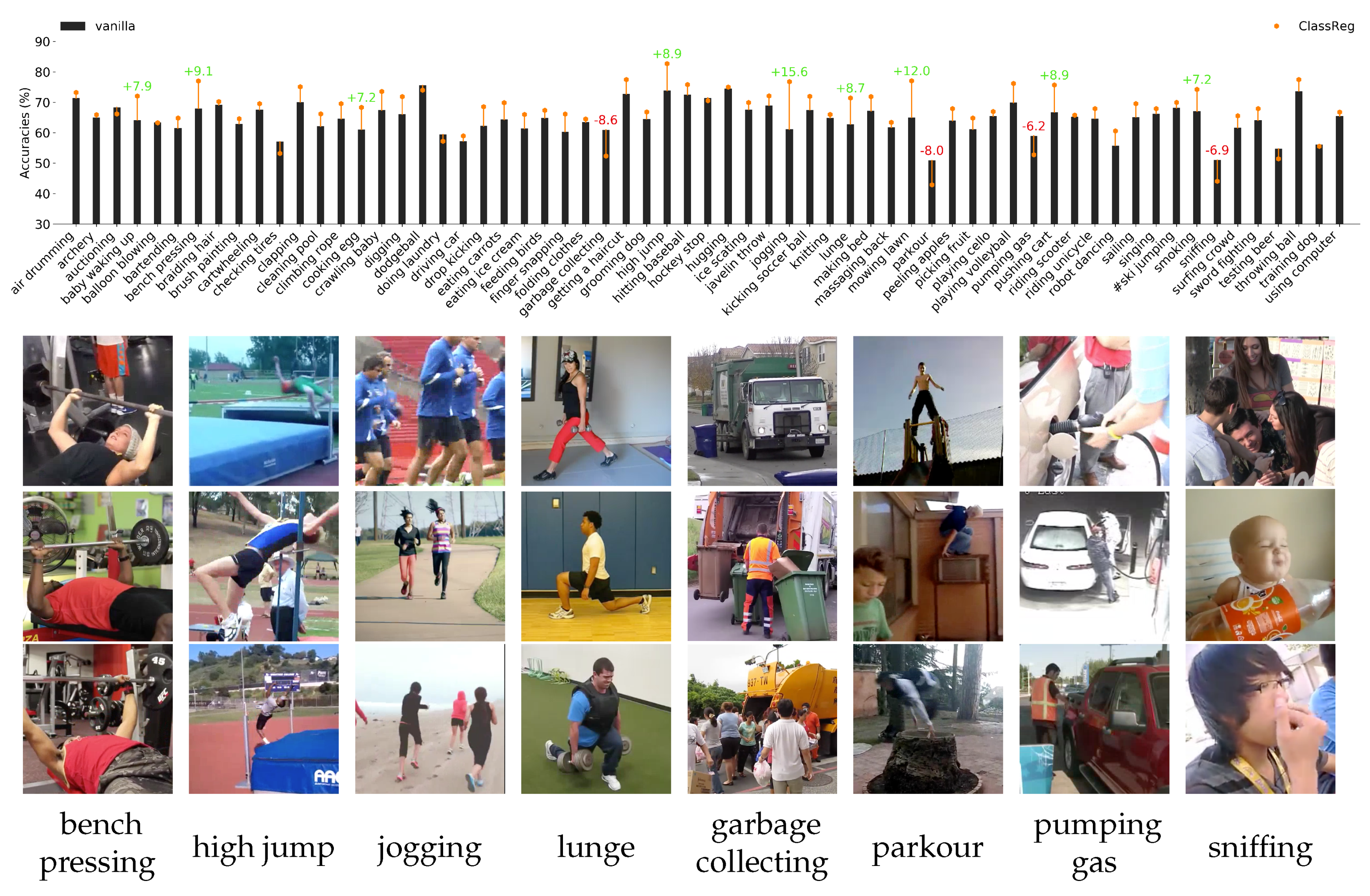
As shown in Figure 5, Class Regularization demonstrates improvements for most classes in Kinetics. The greatest improvements are observed for classes that can be better defined based on their execution instead of their appearance. Examples are “bench pressing“ (9.1% improvement), “high jump“ (8.9% improvement), and “jogging“ (15.6% improvement). Amplifying features that are characteristic of those classes improves the model’s recognition capabilities. In contrast, classes that are more likely to contain significant variation in feature values are more prone to be classified wrongly. This is particularly true for classes that exhibit large intraclass variation, such as “parkour“, where there are no standard actions performed. Other examples are “garbage collection“ in Figure 5 which could be performed either mechanically (top), by a single person (mid), or by multiple people (bottom). Other examples include either oscillations as in “pumping gas“, or require contextual information as in “sniffing“.

4.3. Resulting Statistical Significance

To analyze whether the classification performance with the addition of Class Regularization to a network is statistically relevant, we perform a McNemar’s test on UCF-101 and HMDB-51. We study if the difference in accuracy between a network with and without Class Regularization is to be attributed to marginal homogeneity (i.e., the result of sampling distribution) or if the variance is significant enough to conclude that the two models indeed perform differently. (

Table 4. McNemar’s statistical significance test on the first split of UCF-101 and HMDB-51. Results with and without regularization for (a) ResNet101, (b) Wide-ResNet, and (c) I3D models. (d–f) present results for class-regularized ResNet101 across different blocks in the architecture.

a–c) summarize the McNemar tests, defined in Equation (2), where b are the cases in which the nonregularized model (¬Reg) is correct (+) and the regularized (Reg) is wrong (-), and c are the cases in which the nonregularized model is correct while the regularized is wrong.

$$x^2=\frac{{(b-c)}^2}{b+c}\left\{\begin{array}{c}{H}_0:P_b=P_c\hfill \\ H_1:P_b\ne P_c\hfill \end{array}\right.$$

(2)

We notice that in each of the tested architectures, the c values were significantly larger than those of b. In particular, a standard 3D ResNet-101 model with class regularization is different than that of a model without, with $x^2$ values of 2.48 and 2.84 for UCF-101 and HMDB-51, respectively. For both datasets, the average probability that the difference between the model with and without is attributed to statistical error is approximately 10%. The difference is also evident in architectures that include a larger number of extracted features per layer. This can be seen from the results of the Wide-ResNet-50 model, in which the $x^2$ values are 3.40 and 3.08 for UCF-101 and HMDB-51, respectively. The difference is statistically significant at the $p=0.05$ level. The final comparison considers I3D as the base network to also account for cases of convolution operations being split to multiple and differently sized cross-channeled convolutions. The probability that the measured difference is not due to a systematic difference in performance is approximately 10%. The sum of (b, c) values in every case is reasonably large in order to sufficiently approximate $x^2$ and to conclude that marginal probabilities for models with and without Class Regularization are not homogeneous.

Finally, we compare the class predictions found by the Class Regularization method in different blocks within the architecture in (Table 4d–f). These panels provide an overview of how different depths of the network perform for the given task by gradually ablating blocks of convolutions. As observed for both datasets, the largest change in performance is in the third convolution block (Table 4e), with the transition of information from the third to the fourth block of convolutions (Table 4f) only accounting for a small change in performance based on c. We use this to further demonstrate the merits of Class Regularization as a quantitative way of understanding the informative parts of the overall network, complementing the class-specific feature visualizations.

5. Conclusions

We have introduced Class Regularization, a method that focuses on class-specific features rather than treating each convolution kernel as class-agnostic. Class Regularization allows the network to strengthen or weaken layer activations based on the batch data. The method can be added to any layer or block of convolutions in pretrained models. It is lightweight, as the class weights from the prediction layer are shared throughout Class Regularization blocks. To avoid the vanishing gradient problem and the possibility of negatively influencing activations, the weights are normalized between a range given an affection rate value.

We evaluated the proposed method on three benchmark datasets: Kinetics-400, UCF-101, and HMDB-51; and three models: ResNet101, Wide ResNet50, and I3D. We consistently show improvement when using Class Regularization, with a performance gain of up to 2.45%. The achieved improvements were done with minimal additional computational cost over the original architectures. We also perform a statistical significance test to demonstrate that the outcomes of the different models are indeed based on the additional regularization, rather than being the result of incidental sampling.

Class Regularization can also aid in improving the explainability of 3D-CNNs. Qualitative visualizations reveal which spatiotemporal features are strongly correlated with specific classes. Such analyses can be made for specific layers and, as such, provide insight into the discriminative patterns that specific features represent.

Future works based on Class Regularization should aim towards addressing the feature variations of actions within the same classes, with a greater focus towards the temporal domain. The inclusion of global information and the calibration of local spatiotemporal patterns based on such information, as with Squeeze and Recursion blocks [26], shows a promising direction towards creating spatiotemporal features that can better treat the variations of human actions and interactions.