The Application and Improvement of Deep Neural Networks in Environmental Sound Recognition

Featured Application

Authors are encouraged to provide a concise description of the specific application or a potential application of the work. This section is not mandatory.

Abstract

Neural networks have achieved great results in sound recognition, and many different kinds of acoustic features have been tried as the training input for the network. However, there is still doubt about whether a neural network can efficiently extract features from the raw audio signal input. This study improved the raw-signal-input network from other researches using deeper network architectures. The raw signals could be better analyzed in the proposed network. We also presented a discussion of several kinds of network settings, and with the spectrogram-like conversion, our network could reach an accuracy of 73.55% in the open-audio-dataset “Dataset for Environmental Sound Classification 50” (ESC50). This study also proposed a network architecture that could combine different kinds of network feeds with different features. With the help of global pooling, a flexible fusion way was integrated into the network. Our experiment successfully combined two different networks with different audio feature inputs (a raw audio signal and the log-mel spectrum). Using the above settings, the proposed ParallelNet finally reached the accuracy of 81.55% in ESC50, which also reached the recognition level of human beings.

1. Introduction

We live in a world surrounded by various acoustic signals. People react from their sense of hearing in situations like passing streets, finding someone in a building, or communicating with others. The development of computer vision has given machines the ability to support our lives in many ways. Hearing sense, as another important factor of our lives, is also an appropriate target to develop with artificial intelligence. A machine assistance acoustic detection system could be applied in several aspects, such as healthcare [1], monitoring [2], security [3] and multi-media applications [4].

In the artificial intelligence domain, neural networks have been a popular research field in recent years. Many acoustic topics have been researched with this technique, such as speech recognition [5,6] and music information retrieval (MIR) [7,8]. However, this kind of acoustic research only work for a certain purpose. Unlike this kind of content, the general acoustic events in our lives might not have periodicity or clear rhythms that can be detected, and the non-stationary properties of environmental sound make this problem difficult and complex. To achieve a system that can deal with general acoustic cases, the first step might be to recognize the current environmental scene. Scenes such as coffee shops, streets, and offices all have a unique event set; by adding the scene information into the detection system, the system complexity could be reduced. This is why environmental sound recognition techniques are important and essential.

This study attempted to provide an end-to-end solution for an environmental sound recognition system. There were two major contributions from this research. First, we improved the performance of the network feed with a raw audio signal. Second, we proposed a more flexible parallel network that could combine several kinds of features together. The result showed that this kind of network could combine raw audio signals and the log-mel spectrum efficiently.

The rest of this paper is organized as follows: In Section 2, we introduce the background of this research, including the current research on environmental sound recognition and the fundamental knowledgement of neural networks. In Section 3, a detailed description of our network and development methods is introduced. In Section 4, we perform experiments to examine our network architecture and the proposed development method, and we compare our results with those of other research, using a number of public datasets. In Section 5, we present a conclusion of our work and provide suggestions for further research.

2. Related Works

2.1. Environmental Sound Recognition

The intention of the study is to resolve the conditions around Environmental sound recognition (ESR), which is also known as environmental sound classification. The study is not specifically intended to detect the event trigger time precisely, but more important to understand what the acoustic scene is. In past years, numerous methods, such as the Gaussian Mixture Model (GMM) [9], Hidden Markov model (HMM) [10,11], random forest [12], and support vector machine [13], etc., have been used to solve the ESR problem. However, none of these methods can reach the level of human beings. Since 2012, neural networks have shown the great potential in computer vision [14]. Increasingly, researchers have begun to apply neural networks in the ESR field.

For a neural network, it is important to choose a suitable feature to be the input value. In 2014, Piczak [15] proposed a usable network structure using the log-mel spectrum and delta as the input features, which was once considered state-of-art in the ESR field. The log-mel spectrum has been a popular feature used in the ESR field in recent years. In Challenge on Detection and Classification of Acoustic Scenes and Events (DCASE challenges) [16,17], most of the researchers still choose to take the log-mel spectrum as one of the network inputs in acoustic scene classification tasks.

In 2015, Sainath et al. [6] used a raw audio wave as the network input to train for speech recognition and had promising results. Raw signals seem to be one of the choices in the ESR field.

In 2016, Aytar et al. [18] proposed SoundNet, which is trained using both images and raw audio. The image part is used to assist in the training, but the scene is still recognized according to the raw audio signals. The result of the network was impressive. Although, the performance might drop considerably, the network structure can still be trainable using the raw audio signal only. In the same year, Dai et al. [19] proposed an 18-layer network that could also work with raw audio signals, and the larger number of filters and a deeper structure provided a much better result using raw audio signals. We could clearly see that network architecture has a huge effect with the raw signal input when comparing these two works [18,19]. The depth and the filter numbers are obviously worth further discussions. On the other hand, both the two works use the global pooling strategy [20] to integrate the network output information, which has shown an outstanding effect on dimension reduction. Global pooling has other benefits in structure integration, which is explained in our method development.

In 2017, Tokozume and Harada [21] proposed EnvNet, which transforms a signal from a raw 1d signal to a 2d spectrogram-like graph through the network. This is an interesting idea, because training with a spectrum might also be adapted to this kind of graph. In the same year, Tokozume et al. [22] proposed another augmentation method that could be applied in the same kind of network, and the results could even reach the level of human beings.

These related works reveal that the input features greatly influence the performance of a network. Although many features have been tried on the network, a proper way to combine individual acoustic features are lacking. Moreover, network architectures that use raw signals as the input also require further discussion. Therefore, based on the existing research, this study focuses on improving the above-mentioned aspects.

2.2. Review of Neural Networks

The concept of neural networks has been proposed for a long time [23]. However, it was not considered useful due to the enormous computation requirements. The recent development of computer hardware has given researchers new opportunities to apply the technique in various problems, such computer vision [14] and speech recognition [5], etc. Neural networks show great potential in these aspects. In the following sections, we introduce the fundamental concepts of a neural network, as well as some techniques to tune up a network.

2.3. Feed-Forward Neural Network

The simplest feed-forward neural networks would be Single-layer perceptrons, which can be built up to do a regression. Assume we would like to project a $\mathcal{X} ϵ {\mathbb{R}}^n$ to $\mathcal{Y} ϵ {\mathbb{R}}^m$, the two variables could be rewrite as two vectors $\underset{\_}{\mathcal{X}}= {\left[{𝓍}_1 \cdots {𝓍}_n\right]}^T$ and $\underset{\_}{\mathcal{Y}}= {\left[{𝓎}_{1 \cdots } {𝓎}_m\right]}^T$, so we could simply try the formula below:

$$\underset{\_}{\mathcal{Y}}=\mathrm{W}\underset{\_}{\mathcal{X}}+\mathrm{b}.$$

(1)

In (1), $\mathrm{W} ϵ {\mathbb{R}}^{m \times n}$ and $\mathrm{b} ϵ {\mathbb{R}}^{m \times 1}$, therefore, the main purpose to solve the equation is to find the suitable w and b. If we already had a certain sample ${\mathcal{S}}_i=\left({\mathcal{X}}_i,{\mathcal{Y}}_i\right)$, obviously, we make the result of input ${\mathcal{X}}_i$ could be as close to ${\mathcal{Y}}_i$ as possible. There are several methods that can be used to retrieve the correct value of w and b, such as the stochastic gradient descent (SGD) or Newton’s method. No matter which method is applied, the equation will have a good result when $\underset{\_}{\mathcal{X}}$ and $\underset{\_}{\mathcal{Y}}$ among all the samples are linearly dependent. Inspired by the animal neuron system, the activation function $\phi$ was added to improve Equation (1), and the new equations are listed as (2) and (3):

$$\underset{\_}{\mathsf{\nu }}=\mathrm{W}\underset{\_}{\mathcal{X}}+\mathrm{b}$$

(2)

$$\underset{\_}{\mathcal{Y}}=\mathsf{\phi }\left(\underset{\_}{\mathsf{\nu }}\right).$$

(3)

The activation function provides a non-linear transform to filter out the weaker signal. For example, the classic activation function sigmoid is:

$$\mathrm{sigmoid}\left(\mathrm{x}\right)=\frac{1}{1+e^{-x}}.$$

(4)

After passing Equation (4), every output value is straightly normalized to a range between 0 and 1, which is a superior non-linear transform. Equation (3) can now have the ability to make a regression to the non-linear equation.

From Equation (3), it can be clearly seen that each element in $\underset{\_}{\mathcal{Y}}$ is actually composed of every element of $\underset{\_}{\mathcal{X}}$ in different weights. Here, $\underset{\_}{\mathcal{X}}$ form an input layer, and each node create an element of $\underset{\_}{\mathcal{Y}}$ is called a neuron in the network.

To enhance the network structure, a hidden layer can be added to improve the network performance. The neuron numbers in the hidden layer needs to be decided by users, it usually setup to the value bigger than both input and output dimensions. The hidden layer is used to project the input vector into another dimension, resulting in a greater chance of finding a linear way to transform from a higher dimension to the output layers. Several non-linear transform also make the network hold greater power to complete complex regression.

To obtain the correct weights of the feed-forward neural networks, the backpropagation method [24] (BP) is widely used. By calculating the gradient from the loss function, the gradients can be backward propagated to each of the weights.

It seems that the network would better be design deeper, more layers, or wider, more neurons per layer, but actually both of the two methods all get some issues need to be deal with. The weight number grows exponentially with the width of the network, which also leads to a large growth of the computation times and also causes the network to face a serious overfitting condition. This also means that the network might easily fit the training data but still result in poor performance while testing. Deeper networks need to solve the gradient decent problem. When performing BP, the gradient travels from the end of the network and gets thinner and thinner while arriving at the front, and it can even vanish directly. A number of methods have been proposed to improve the vanishing gradient problem, of which a deeper network is recommended to be built as a solution.

2.4. Convolutional Neural Networks

The convolutional neural network (CNN) is a special type of neural network used in image recognition. LeNet [25] is considered to be the first complete CNN. It is composed of convolution layers, activation layers, pooling layers, and fully connected layers. These layers all have special usages, which are introduced later in the paper. CNN resembles the original input image into a series of feature maps, by which each pixel in the feature map is actually a neuron. Unlike the way in which a normal neural network acts, each neuron does not connect to all the neurons in the previous layer; the connections only build up when these two neurons have a certain locality relationship. It makes sense because the information revealed in a certain location intuitively has a little chance to be related to another distant location. In this way, the total weight is reduced, which helps to improve the over-fitting condition.

2.5. Convolutional Layers

Each convolutional layer is composed of several graphic filters called kernels, it works just like the way in image processing does. Through convolutions, the kernels enhance part of the image’s characteristic and turn the image into an individual feature map. The feature maps are all the same size and are bundled together to become a brand-new image. The convolutional layer provides an example regarding what the new image will look like. Each map in the same image is called a channel, and the number of channels becomes the depth of the image. When working through the convolution layers, the kernel actually processes all the channels once at a time. Another important aspect of the convolutional layer is parameter sharing. If we look back to the processing method of MLP, we can discover that each pixel in the same image needs to be applied to different kernels. However, in convolutional layers, the whole image shares the same kernel to create a feature map, which gives CNN an important shift invariant characteristic. As the kernel can move all around the image, the features correlated with the kernel can be detected anywhere, which gives CNN superior performance in image recognition.

2.6. Activation Layers

As mentioned in the previous section, the main purpose of the activation layer is to provide a non-linear transform. These functions need to be derivative. There are several types of activation functions, including sigmoid (4), tanh (5) and rectified linear unit (ReLU) (6):

$$\tanh \left(\mathrm{x}\right)= \frac{e^x-e^{-x}}{e^x+e^{-x}}$$

(5)

$$\mathrm{ReLU}\left(x\right)=max\left(x,0\right).$$

(6)

Unfortunately, these activation functions all have some flaws. When using the gradient decent methods, ReLU can be affected by gradient exploding, because ReLU does not change the range of the output value from the input. Another problem cause by ReLU is the dead ReLU problem. When a relu has a negative input value, it will give an output of 0, which will cause the whole chain of the input to not update at that time, or even worse, never update until training is finished. On the other hand, sigmoid and tanh are affected by the vanishing gradient problem, because the gradients BP from these functions will at most only have 1/4 left. Comparing with these two groups of activation functions, we observe that the problem of ReLU can be solved by adding a normalization layer, which also results in a faster processing speed. For these reasons, ReLU is now the most commonly-used activation function.

2.7. Pooling Layers

Even though parameter sharing reduces the large number of parameters for CNN, for a large-scale picture, it is still necessary to find a reasonable way to perform subsampling. Pooling layers can be used to finish this job.

For a continuous signal (like an image), it is intuitive to perform downsampling by grouping a fixed number of adjacent values and then picking up an output value from each group. The pickup method could be based on the average, maximum, or minimum. Among these methods, maximum pooling has shown the best result and is commonly used now.

However, care must be taken, as not all feature maps can take pooling as the down sampling method. According to the previous description, each value in the same group needs to be adjacent, which means these values actually have some spatial relationships, and each group also needs to have the same spatial meaning. Therefore, pooling layers might not be suitable to in some cases using CNN, such as in game maps [26].

2.8. Fully Connected Layers

Fully connected (FC) layers are similar to the typical MLP. The processing feature maps are flattened before entering this layer and transform from several dimensions to a single vector. Most of the parameters in a CNN are set in FC layers, and the size of the FC layer determines the capacity of the network.

2.9. Loss Function

A neural network can be used for classification and regression, each of which needs a different loss function, and these functions all need to be derivate:

$$Los{s}_{mse}\left(\underset{\_}{y},\underset{\_}{t}\right)=\frac{1}{2}{\left(\underset{\_}{y}-\underset{\_}{t}\right)}^2.$$

(7)

Equation (7) is the mean square loss (MSE) function, which is often used in regression tasks. It directly shows the difference between the output value and the target value. Another loss function often used in classification is cross entropy, which usually works with the softmax logistic function. In Equation (7), $\underset{\_}{y}= {\left[y_1 \cdots y_J\right]}^T$ is the output vector coming from the FC layer and the J is the final class number. Softmax tends to find the probability distribution of the classification result. After passing through the function, the sum of output vector $\underset{\_}{S}$ becomes 1, and $S_j$ represents the probability of the input being classified as class j:

$$S_j\left(\underset{\_}{y}\right)= \frac{e^{y_j}}{{{\displaystyle \sum }}_{k=1}^J{e}^{y_k}}$$

(8)

$${\mathrm{Loss}}_{cross entropy}\left(\underset{\_}{y},\underset{\_}{t}\right)= -{\displaystyle \sum }_{j=1}^J{t}_{j}log{S}_j\left(\underset{\_}{y}\right)$$

(9)

$${\mathrm{Loss}}_{cross entropy}= -log{S}_j\left(\underset{\_}{y}\right).$$

(10)

The purpose of cross entropy is to estimate the difference between two vectors by calculating the log likely-hood function. The result is the same as that shown by Equation (9). In most classification cases, the final result will be a one-hot vector, in which target j has a value of one and the other element is zero, that is, only $S_j$ has the value. Therefore, the loss function then be simplified to (10).

2.10. Model Initialization

In a network, there are numerous hyper parameters that need to be decided, it is normally to consider a way to do the initialize. An ideal properly-initialized network could have the following property: if we take a series of random inputs into the network, the output should be fairly distributed in each of the classes, and there should not be any particular trends at the beginning. Obviously, randomly initializing the parameters will not have this effect. Glorot and Bengio proposed normalized initialization [27] to keep the various from the layer input to output.

$$\mathrm{W} ~ \mathrm{U} \left[ -\frac{\sqrt{6}}{\sqrt{n_j+n_{j+1}}} , \frac{\sqrt{6}}{\sqrt{n_j+n_{j+1}}}\right]$$

(11)

$n_j$ in Equation (11) means the number of inputs in layer j. Equation (11) performs well for linear layers, but for nonlinear layers like ReLU, the equation needs to be adjusted.

He et al. proposed another method [28] to fix the formula, in which $n_{j+1}$ in (11) can be simply ignored. Our experiment used He’s method to initialize the network.

2.11. Batch Normalization

In the previous section, it was mentioned that ReLU needs a method to support it in arranging the output value. The distribution of the output value also needs to be controlled. Sergey et al. proposed a method called batch normalization [29]. The main concept of this method is to force the addition of a linear transform before the nonlinear layer to make the variance and mean of the nonlinear layer input ${\rm X}, {\rm X}ϵ {\mathbb{R}}^{i \times j \times k}, i+j+k=m$ be in a certain range:

$${\mu }_{\beta } \leftarrow \frac{1}{m}{\displaystyle \sum }_{i=1}^m{x}_i$$

(12)

$${\sigma }_{\beta }^2 \leftarrow \frac{1}{m}{\displaystyle \sum }_{i=1}^m{\left(x_i- {\mu }_{\beta }\right)}^2$$

(13)

$$\widehat{x_i} \leftarrow \frac{x_i- {\mu }_{\beta }}{\sqrt{{\sigma }_{\beta }^2+\in }}$$

(14)

In Equations (12) and (13), the value of m is the total number of elements in the mini-batch and channels. After Equation (14), the purpose is to find the current mean value ${\mu }_{\beta }$ and current variance ${\sigma }_{\beta }$, and then adjust them to become 0 and 1:

$$y_i \leftarrow \gamma \widehat{x_i}+ \beta \equiv B{N}_{\gamma ,\beta }\left(x_i\right).$$

(15)

Other learnable transform parameters can be added into the formula, and the final result will be similar to Equation (15). These two variables help the input values to do a little bit adjustment, which helps to solve the dead ReLU problem. It is essential to take batch normalization in a deep network.

3. Method Development

3.1. Data Sets

In our experiments, we took two kinds of public data sets to evaluate our network structure improvements: ESC50 [30] and ESC10 (Warsaw University of Technology, Warsaw, Poland).

ESC50 is a collection of environmental sound recordings that contains 50 classes, such as airplanes, car horns, cats, humans laughing, and rain, etc. There are 2000 short clips in total, and each class has 40 files. Each clip is five seconds long, and there is a total length of 2.78 h. It was recommended to test with the official 5-fold setting, as some of the files in the same class are extracted from the same source, using the official fold could avoid some problems.

ESC10 is a subset of ESC50 that takes out 10 classes from ESC50, while other configurations remain the same. It was beneficial to do a small-scale test in this dataset first.

3.2. Data Preprocessing

There are three kind of data put into our CNN such as the raw signal, the mel-spetrogram, and the output of 1D network. The output of 1D network is that we input signal into the 2D network. For the preprocessing, we first down-sampled the audio files to a sample rate of 16,000, averaged the stereo audio to mono, and eliminated the empty segments at the front and the tail of the files. If the resulting file was less than 1.5 s, we equally filled up the length with the 0 value at the beginning and end of the files. In the training phase, based on the method in [22], we appended 750 ms of 0 to both sides of the audio and then randomly cropped a 1.5 s clip, while the variance of the clip was 0. We then continued to repeat the procedure. After cropping the file, the mean and variance of the clip were normalized to 0 and 1. In the testing phase, we sequentially cropped 10 clips of 1.5 s each from the test audio. Each clip overlapped for about 390 ms. We chose the majority of probability scheme to do the final classification for each test file.

For the log spectrum, we transferred from the normalized clip with a sample rate of 16,000. The frame size was set to 512 (about 30 ms) with a 50% overlap, and the resulting values were then put through the log operation and mel-filters. This finally resulted in a 128-bin mel-spectrum. We did not make further normalizations to the spectrum graph, and they were fed into the network directly.

3.3. Data Augmentation

Compared to image datasets [31,32], acoustic datasets are not very popular; the number of files is insufficient, and there is a lack of diversity. Some researches [22,33] have revealed that data augmentation can help to enhance the result of classification. Common acoustic augmentation methods include pitch shifting and time stretching. Although CNN is shift invariant, these augmentation methods still have an effect on network training, therefore we chose both of them to be our augmentation methods.

We performed another augmentation method, known as wave overlapping, which was inspired by the study in [22] and their use of between class learning. We simplified the method to perform augmentation for just for a signal class. We, first, randomly cropped two segments of the same size from a single file, and then multiplied each of them by an individual random ratio from 0 to 1. These two crops were then summed up together, and the mean and variance were normalized to 0 and 1. The difference of volume we create for the new segment riches the diversity of the data. It is a simple method to enhance the dataset, and keeps the labels unchanged. The result shows that it is even better than just provide two of the individual crops. The experiment is described in the following chapter.

3.4. Network Customization

CNN provides a flexible method to extract features from any kind of input. Many researches [18,19,21,22] have shown that raw signals can be the input of a network. Inspired by [21], we assumed that the concatenation of a 1d feature map would form a spectrum-like graph. In fact, the 1d convolution along the time axis could actually fetch the frequency information from the raw signal. Each channel represents a set of frequencies, and the Y axis of the concatenation map means the frequency sets the response at a certain moment. We believed that more features could be extracted from this kind of map. Therefore one of our purposes was to optimize the extraction network. As shown in Figure 1, we proposed a network structure feed with raw signals and output a feature vector to entering a full connected layer to do the classification.

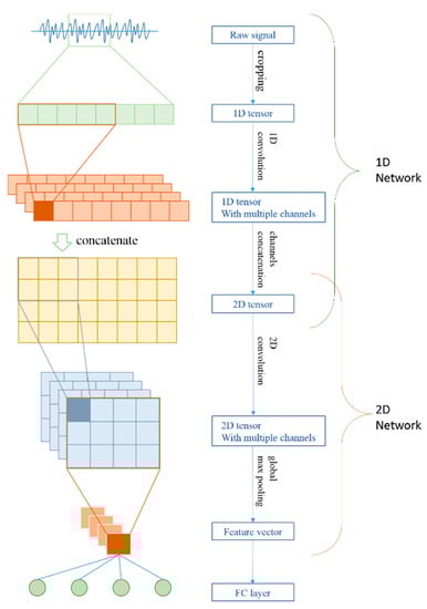
Figure 1. Network structure for ESR classification. The 1D and 2D networks are serialized together but could also work alone to be fit with different situations.

The network was composed of a 1D and 2D network. Just like the description above, the 1D network was used to extract a spectrum-like map, and the 2D network was used to find detailed features from the map.

Furthermore, the 2D network could not only be used in our network-organized map but could also be applied in the mel filter bank spectrum. In the next chapter. We would show the result of our network processing these two kinds of feature maps. Our network architectures are listed in Table 1 and Table 2.

Table 1. Architecture of the 1D network.

Layer	Ksize	Stride	Padding	#Filters
Input (1 × 24,000)
Conv1	13	1	same	32
Pool	2	2	0	--
Conv2	13	1	same	64
Conv3	15	3	same	128
Conv4	7	5	same	128
Conv5	11	8	same	128
Channel concatenation (1 × 128 × 100)

Table 2. Architecture of the 2D network and full connections.

Layer	Ksize	Stride	#Filters
Input (1 × M × N)
3 × Conv (1~3)	(15, 1)	(1, 1) (1, 1) (1, 1)	32
3 × Conv (4~6)	(15, 1)	(1, 1) (1, 1) (2, 1)	64
3 × Conv (7~9)	(15, 1)	(1, 1) (1, 1) (2, 1)	128
3 × Conv (10~12)	(5, 5)	(1, 1) (1, 2) (2, 2)	256
3 × Conv (13~15)	(3, 3)	(1, 1) (1, 1) (1, 1)	256
3 × Conv (16~18)	(3, 3)	(1, 1) (1, 1) (1, 1)	512
Conv19	(3, 3)	(2, 2)	512
Conv20	(3, 3)	(1, 1)	1024
Global max pooling (1024)
FC1 (2048)
FC2 (# classes)

In Table 1, Conv refers to the convolutional layers and Pool refers to the max pooling layers. All the Conv layers were appended with a batch normalization layer and a ReLU layer. The input tensor of the network was a 1d tensor of 1 × 24,000 (a 1.5 s clip under a sample rate of 16,000), and the output tensor was a 2d tensor of 1 × 128 × 120.

In Table 2, the first six blocks contained three Conv layers each. These three Conv layers had the same kernel size and filter number, but were constructed with different stride settings. All the Conv layers were appended with a batch normalization layer and a ReLU layer. FC1 was also followed by a batch normalization layer, a ReLU layer, and a drop out [34] for 50%. Padding was always applied on Conv layers, and if there was no stride, the size of the output would be the same as the input of each layer. The input size of this network was adjustable, but due to global pooling, the output size of the max pooling layers could be controlled as the last channel number, which was 1024 in Conv 20.

3.5. Network Parallelization

One of the main purposes of our work was to find a suitable method to combine several features in the network, we desired these features could eventually help adjust other networks during the training procedure. Applying the idea to the features with high homogeneity is intuitive. Based on our 1D and 2D networks, we proposed a feature parallel network and took raw signals and the mel-spectrum as examples. Figure 2 represents the concept of our method. In the last layer of the two-dimensional (2D) network, we used the global max pooling [20] to extract the feature vector from different kinds of feature maps. These extracted vectors could easily connect along the same axis whether their length being the same or not. In our experiment, we tested the parallel features using the same vector size of 1024; therefore, the length of the 1d tensor entering the FC layer shown in Figure 2 was 2048.

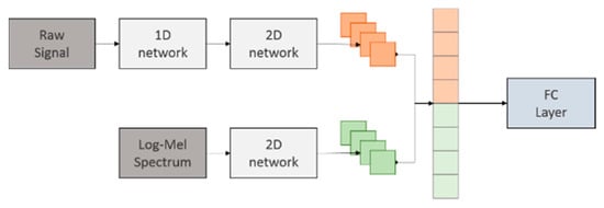
Figure 2. Parallel architecture of the network.

4. Results and Discussion

4.1. Experiment Setup

The neural network could be highly complex, but have only a few non-linear layers. The increasing of the depth makes the network easier to fetch the abstract expression form the source. Our intention of increasing the depth of the network allows the network to generate an effective acoustic filter, like mel-filter from signal processing.

We were interested in some particular setting within the network, so we would like to try modify some of these settings to examine what would they take effect. Our experiment focused on the following topics:

• Signal length per frame in the 1D network
• Depth of the 1D network
• Channel numbers of the 1D network (the height of the generated map)
• Kernel shape in the 2D network
• The effect of pre-training before parallel
• The effect of the augmentation

We took ESC50 and ESC10 as our datasets, and used the official fold settings. The experiments only consisted of training and testing, and we did not perform additional validations. Each experiment ran for 350 epochs, and we used Nesterov’s accelerated gradient [35] as our network optimization method. The momentum factor was set to 0.8. The initial learning rate was set to 0.005 and decayed to 1/5 in the following epochs: 150 and 200. L2 regulation was also used and was set to 5 × 10⁻⁶. Our models were built using PyTorch 0.2.0 and were trained on the machine with GTX1080Ti (NVIDIA, Santa Clara, CA, USA). The audio wav files were extracted using PySoundFile 0.9, and LibROSA 0.6 was used to create the mel-spectrums.

4.2. Architecture of the 1D Network

To test the influence of the filter size in the 1D network, it was necessary to slightly modify the network structure shown in Table 1.

The kernel sizes of Conv 4 and Conv 5 in the 1D network affected the frame length the most, therefore we tried three kinds of combinations to reach 25 ms, 35 ms, and 45 ms per frame. Test accuracy with the different frame lengths setting: the frame indicates the output unit of the 1D network. The dataset used in this test was ESC50, as shown in Table 3.

Table 3. Test accuracy with different frame length settings.

Frame Length	~25 ms	~35 ms	~45 ms
ksize of Conv4	7	15	21
ksize of Conv5	11	15	19
Avg.	73.55%	72.45%	72.55%
Std. dev.	2.89%	2.57%	1.54%

Clearly, the most stable result was found at a frame size of 25 ms; as the frame size increased, the accuracy worsened. The result found at 25 ms showed the most generalizability.

4.3. Network Depth

In the depth test, the epochs times is 350, but the result always converged before the 350 epochs. Increasing the depth of the network could enhance the non-linear transform ability of the network, and it is known as to enrich the abstract expressiveness. Also, the non-linear transform could consider as the processes to form the acoustic filter just like mel-filter, gammatone-filter, etc.

In this test, we inserted a certain number of layers before Conv 2–5. The settings of these layers were ksize = 3 and strides = 1. Padding was introduced to maintain the input length, the filter numbers were equal to the former Conv layer, and each of the insertion layers was followed by a batch normalization layer and a ReLU layer. The distribution of these layers was considered to not significantly affect the frame length. We get two kinds of setting, 12 or 24 additional layers, the location means in front of where these layers would be put. The configuration is shown in Table 4, and the result in Table 5.

Table 4. Configuration of the depth test.

	#Layers	Distribution of 12 Layers	Distribution of 24 Layers
Location
Conv2		6	10
Conv3		3	8
Conv4		2	5
Conv5		1	1

Table 5. Test accuracy with different depth settings of the 1D network.

Depth	12 + 5	24 + 5
Avg.	72.00%	66.95%
Std.	1.28%	2.62%

Although parameter numbers of the network increased slightly, we found that the network could still converge within 350 epochs, so we kept it the same.

It was surprising that the depth of the 1D network did not significantly affect the result, or even worse, the results going down while the network becomes deeper. The results were not consistent with that of Dai et al. [19]. The main reason for this discrepancy may have been due to the frame size in their experiment but not the depth of the network. More researches and experiments may be needed to prove this argument.

4.4. Number of Filters

A sufficient number of filters was necessary to provide sufficient capacity for the network to load the frequency information. Therefore, it could not be set too small. On the other hand, an excessively large setting would cause a large graph to pass into the 2D network, which would slow down the network processing but not provide a significant improvement in accuracy. We tried three different settings: 64, 128, and 256, and the result is shown in Table 6.

Table 6. Test accuracy using different filter numbers in the 1D network.

#Filters	64	128	256
Avg.	71.05%	73.55%	74.15%
Std.	2.05%	2.89%	3.16%

Although the setting of 256 had a slightly better result than 128, it required almost three times the amount of training compared with the 128 filters model, we chose 128 filters as our final decision.

4.5. Architecture of the 2D Network

The kernel shape could affect the invariant shifting of CNN, and it is not desired for this kind of invariant characteristic to show up in the frequency domain. In fact, a square kernel has been proven to not be suitable for spectrum content. We tried three different shape settings to see which would the best performer using our 1D-2D network by modified the size value of Conv (1~9). The test result is shown in Table 7.

Table 7. Test accuracy using different kernel shapes in the 2D network.

Size	(15,1)	(15,15)	(1,15)
Avg.	73.55%	67.25%	70.85%
Std.	2.89%	2.57%	2.75%

4.6. Parallel Network: The Effect of Pre-Training

To achieve the best performance of the parallel network, a pre-training procedure was required. Our network was composed of a raw-signal-1D-2D network, a spectrogram-2D network, and a set of fc layers. The pre-training procedure was built on the first two parts individually with their own fc layers (see Figure 1), trained the network alone, and then took over the essentials part and connected them into the parallel network. Likewise, we added an additional data source to improve the network analysis capability. These two data sources with high homogeneity are chosen. The neural network tends to ignore some information during the training, and our adding procedure is additional information, the feature vector from another network, back to it after training. We tried two kinds of the pre-training settings and compared them with the network before pre-training: Only pre-trained the raw-signal-1D-2D network. Both the upper reaches were pre-trained. The result is shown in Table 8.

Table 8. Test accuracy.

Pre-Train Network	Without Pre-Train	Raw Signal Only	Both Network
Avg.	78.20%	75.25%	81.55%
Std.	2.96%	2.18%	2.79%

The worst result occurred when the network was pre-trained only using the raw-signal-input network; however, if we pre-trained both networks, we could then get the best result. This revealed that the trained 1D-2D network could disturb the training procedure of the spectrogram network.

4.7. Data Augmentation

In this section, we test the augment method mentioned in the former paragraph. The wave- overlapping method was used to insert two different crops into a single clip, and then three different kinds of settings were applied. The original ESC50 had 1600 sets of training data in each fold. We randomly picked up certain sets of data to make the additional training clips. Setting 1 took 800 original clips, and Setting 2 took 400 clips. The wave overlapping created two crops from a single original source. Setting 3 caused these two crops to be pitch shifted or time stretched. We tested the result using a partially pre-trained network and a fully pre-trained one. The results are shown in Table 9 and Table 10.

Table 9. Test accuracy of augments applied in partial pre-pertained network.

Aug Type	Original with Extra	Overlap with Raw	Overlap with PS/TS
Avg.	74.05%	76.95%	75.20%
Std.	3.55%	3.59%	2.65%

Table 10. Test accuracy of augments applied in full pre-trained network.

Aug Type	Original with Extra	Overlap with Raw
Avg.	81.40%	81.35%
Std.	3.04%	3.03%

4.8. Network Conclusion

The previous experiments found a network architecture with the most efficient settings. We next compared our results with the networks with other researches based on raw signals or spectrograms without augmentations, as shown in Table 11.

Table 11. Test result of different kinds of models with open-datasets.

Models	Features	Accuracy
		ESC50	ESC10
Piczak’s CNN [15]	log-mel spectrogram	64.5%	81.0%
m18 [19]	raw audio signal	68.5% [22]	81.8% [22]
EnvNet [21] *	raw audio signal ⊕ log-mel spectrogram	70.8%	87.2%
SoundNet (5 layers) [18]	raw audio signal	65.0%	82.3%
AlexNet [36]	spectrogram	69%	86%
GoogLeNet [36]	spectrogram	73%	91%
EnvNet with BC [22] *	raw audio signal ⊕ log-mel spectrogram	75.9%	88.7%
EnvNet–v2 [22]	raw audio signal	74.4%	85.8%
1D-2D network (ours)	raw audio signal	73.55%	90.00%
ParallelNet (ours)	raw audio signal &log-mel spectrogram	81.55%	91.30%
Human accuracy [30]		81.3%	95.7%

* Result combined before softmax.

We summarized our experiment results as following:

• Our proposed method is an end to end system achieving 81.55% of accuracy in ESC50.
• Our proposed 1D-2D network could properly extract features from raw audio signal, compared with the old works.
• Our proposed ParallelNet could efficiently raising the performance with multiple types of input features.

5. Conclusions and Perspectives

This study proposed a 1D-2D network to perform audio classification, using only the raw signal input, as well as obtain the current best result in ESC50 among the networks using only the raw signal input. In the 1D network, we showed that the frame size had the largest effect, and that a deeper network might not be helpful when only using batch normalization. In addition, our parallel network showed great potential in combining different audio features, and the result was better than that for networks taking only one kind of feature individually. The final accuracy level corresponded to that of a human being.

Although we found that different frame size and network depth settings could affect the performance of a 1D network, the reasons causing these phenomena require more studies. Much research [37,38,39] has proposed methods to show the response area in the input graphics of CNN for the classification result or even for certain filters. The deep learning on sequential data processing with Kolmogorov’s theorem is more and more important. Fine-grained visual classification tasks, Zheng et al. [40] proposed a novel probability fusion decision framework (named as PFDM-Net) for fine-grained visual classification. The authors in [41] proposed a novel device preprocessing of a speech recognizer, leveraging the online noise tracking and deep learning of nonlinear interactions between speech and noise. While, Osayamwen et al. [42] showed that such a supervisory loss of function is not optimal in human activity recognition, and they improved the feature discriminative power of the CNN models. These techniques could help find out hot spots in a spectrogram and could also help to generate a highly response audio clip for certain layers, which could provide a good direction for analyzing the true effect behind each kind of setting.

Most of our work focused on the arrangement of a 1D network, and there are still some topics for a 2D network that need to be discussed, such as network depth, filter size, and layer placement. These topics are all good targets for future work.

Our parallel network combined the raw audio input and log-mel spectrum successfully. More input features could also be tried in the future, such as mel-frequency cepstral coefficients (MFCC) and gammatone spectral coefficients (GTSC), etc. The feature vector ratio is also a good topic for future discussion. With the help of global pooling, we could even combine different kinds of network structures to perform the parallel test, just like the diverse fusion network structures used in computer visual. Our parallel methods have excellent research potential.

References

- Chen, J.; Cham, A.H.; Zhang, J.; Liu, N.; Shue, L. Bathroom Activity Monitoring Based on Sound. In Proceedings of the International Conference on Pervasive Computing, Munich, Germany, 8–13 May 2005. [Google Scholar]
- Weninger, F.; Schuller, B. Audio Recognition in the Wild: Static and Dynamic Classification on a Real-World Database of Animal Vocalizations. In Proceedings of the Acoustics, Speech and Signal Processing (ICASSP) 2011 IEEE International Conference, Prague, Czech, 22–27 May 2011. [Google Scholar]
- Clavel, C.; Ehrette, T.; Richard, G. Events detection for an audio-based Surveillance system. In Proceedings of the ICME 2005 IEEE International Conference Multimedia and Expo., Amsterdam, The Netherlands, 6–8 July 2005. [Google Scholar]
- Bugalho, M.; Portelo, J.; Trancoso, I.; Pellegrini, T.; Abad, A. Detecting Audio Events for Semantic Video search. In Proceedings of the Tenth Annual Conference of the International Speech Communication Association, Bighton, UK, 6–9 September 2009. [Google Scholar]
- Mohamed, A.-R.; Hinton, G.; Penn, G. Understanding how deep Belief Networks Perform Acoustic Modelling. In Proceedings of the Acoustics, Speech and Signal Processing (ICASSP), 2012 IEEE International Conference, Kyoto, Japan, 23 April 2012. [Google Scholar]
- Sainath, T.N.; Weiss, R.J.; Senior, A.; Wilson, K.W.; Vinyals, O. Learning the speech front-end with raw waveform CLDNNs. In Proceedings of the Sixteenth Annual Conference of the International Speech Communication Association, Dresden, Germany, 6–10 September 2015. [Google Scholar]
- Lee, H.; Pham, P.; Largman, Y.; Ng, A.Y. Unsupervised Feature Learning for Audio Classification Using Convolutional Deep Belief Networks. In Proceedings of the Advances in Neural Information Processing Systems, Vancouver, BC, Canada, 7–10 December 2009. [Google Scholar]
- Van den Oord, A.; Dieleman, S.; Schrauwen, B. Deep Content-Based Music Recommendation. In Proceedings of the Advances in Neural Information Processing Systems, Lake Tahoe, NV, USA, 5–10 December 2013. [Google Scholar]
- Peltonen, V.; Tuomi, J.; Klapuri, A.; Huopaniemi, J.; Sorsa, T. Computational Auditory Scene Recognition. In Proceedings of the Acoustics, Speech, and Signal Processing (ICASSP), 2002 IEEE International Conference, Orlando, FL, USA, 13–17 May 2002. [Google Scholar]
- Rabiner, L. A tutorial on hidden Markov models and selected applications in speech recognition. Proc. IEEE 1989, 77, 257–286. [Google Scholar] [CrossRef]
- Peng, Y.-T.; Lin, C.-Y.; Sun, M.-T.; Tsai, K.-T. Healthcare audio event classification using hidden markov models and hierarchical hidden markov models. In Proceedings of the ICME 2009 IEEE International Conference Multimedia and Expo, Cancun, Mexico, 28 June–3 July 2009. [Google Scholar]
- Elizalde, B.; Kumar, A.; Shah, A.; Badlani, R.; Vincent, E.; Raj, B.; Lane, I. Experiments on the DCASE challenge 2016: Acoustic scene classification and sound event detection in real life recording. arXiv 2016, arXiv:1607.06706. [Google Scholar]
- Wang, J.-C.; Wang, J.-F.; He, K.W.; Hsu, C.-S. Environmental Sound Classification Using Hybrid SVM/KNN Classifier and MPEG-7 Audio Low-Level Descriptor. In Proceedings of the Neural Networks IJCNN’06 International Joint Conference, Vancouver, BC, Canada, 16–21 July 2006. [Google Scholar]
- Krizhevsky, A.; Sutskever, I.; Hinton, G.E. Imagenet Classification with Deep Convolutional Neural Networks. In Proceedings of the Advances in Neural Information Processing Systems, Lake Tahoe, NV, USA, 3–8 December 2012. [Google Scholar]
- Piczak, K.J. Environmental sound classification with convolutional neural networks. In Proceedings of the Machine Learning for Signal Processing (MLSP), 2015 IEEE 25th International Workshop, Boston, MA, USA, 17–20 September 2015. [Google Scholar]
- Stowell, D.; Giannoulis, D.; Benetos, E.; Lagrange, M.; MPlumbley, D. Detection and Classification of Acoustic Scenes and Events. IEEE Trans. Multimed. 2015, 17, 1733–1746. [Google Scholar] [CrossRef]
- DCASE 2017 Workshop. Available online: http://www.cs.tut.fi/sgn/arg/dcase2017/ (accessed on 30 June 2017).
- Aytar, Y.; Vondrick, C.; Torralba, A. Soundnet: Learning Sound Representations from Unlabeled Video. In Proceedings of the Advances in Neural Information Processing Systems, Barcelona, Spain, 5–10 December 2016; pp. 892–900. [Google Scholar]
- Dai, W.C.; Dai, S.; Qu, J.; Das, S. Very Deep Convolutional Neural Networks for Raw Waveforms. In Proceedings of the Acoustics, Speech and Signal Processing (ICASSP), 2017 IEEE International Conference, New Orleans, LA, USA, 5–9 March 2017. [Google Scholar]
- Lin, M.; Chen, Q.; Yan, S. Network in Network. arXiv 2013, arXiv:1312.4400. [Google Scholar]
- Tokozume, Y.; Harada, T. Learning Environmental Sounds with End-to-End Convolutional Neural Network. In Proceedings of the Acoustics, Speech and Signal Processing (ICASSP), 2017 IEEE International Conference, New Orleans, LA, USA, 5–9 March 2017. [Google Scholar]
- Tokozume, Y.; Ushiku, Y.; Harada, T. Learning from Between-class Examples for Deep Sound Recognition. In Proceedings of the ICLR 2018 Conference, Vancouver, BC, Canada, 30 April–3 May 2018. [Google Scholar]
- Rosenblatt, F. The perceptron: A probabilistic model for information storage and organization in the brain. Psychol. Rev. 1958, 65, 386–408. [Google Scholar] [CrossRef] [PubMed]
- Rumelhart, D.E.; Hinton, G.E.; Williams, R.J. Learning representations by back-propagating errors. Nature 1986, 323, 533. [Google Scholar] [CrossRef]
- LeCun, Y.; Bottou, L.; Bengio, Y.; Haffner, P. Gradient-based learning applied to document recognition. Proc. IEEE 1998, 86, 2278–2324. [Google Scholar] [CrossRef]
- Silver, D.; Huang, A.; Maddison, C.J.; Guez, A.; Sifre, L.; van den Driessche, G.; Schrittwieser, J.; Antonoglou, I.; Panneershelvam, V.; Lanctot, M. Mastering the game of Go with deep neural networks and tree search. Nature 2016, 529, 484. [Google Scholar] [CrossRef] [PubMed]
- Glorot, X.; Bengio, Y. Understanding the Difficulty of Training Deep Feedforward Neural Networks. In Proceedings of the thirteenth international conference on artificial intelligence and statistics, Chia Laguna, Italy, 13–15 May 2010. [Google Scholar]
- He, K.; Zhang, X.; Ren, S.; Sun, J. Delving Deep into Rectifiers: Surpassing Human-Level Performance on Imagenet Classification. In Proceedings of the IEEE International Conference on Computer Vision, Las Condes, Chile, 11–18 December 2015. [Google Scholar]
- Ioffe, S.; Szegedy, C. Batch normalization: Accelerating deep network training by reducing internal covariate shift. arXiv 2015, arXiv:1502.03167. [Google Scholar]
- Piczak, K.J. ESC: Dataset for Environmental Sound Classification. In Proceedings of the 23rd ACM international conference on Multimedia, Brisbane, Australia, 26 October 2015. [Google Scholar]
- Deng, J.; Dong, W.; Socher, R.; Li, L.-J.; Li, K.; Fei-Fei, L. Imagenet: A Large-Scale Hierarchical Image Database. In Proceedings of the IEEE Conference Computer Vision and Pattern Recognition CVPR, Miami, FL, USA, 20–25 June 2009. [Google Scholar]
- Lin, T.-Y.; Maire, M.; Belongie, S.; Hays, J.; Perona, P.; Ramanan, D.; Doll’ar, P.; Zitnick, C.L. Microsoft Coco: Common Objects in Context. In Proceedings of the European Conference on Computer Vision, Zurich, Switzerland, 6–12 September 2014. [Google Scholar]
- Salamon, J.; Bello, J.P. Deep convolutional neural networks and data augmentation for environmental sound classification. IEEE Sign. Process. Lett. 2017, 24, 279–283. [Google Scholar] [CrossRef]
- Srivastava, N.; Hinton, G.; Krizhevsky, A.; Sutskever, I.; Salakhutdinov, R. Dropout: A simple way to prevent neural networks from overfitting. J. Mach. Learn. Res. 2014, 15, 1929–1958. [Google Scholar]
- Nesterov, Y. Gradient Methods for Minimizing Composite; Springer: Berlin/Heidelberg, Germany, 2007. [Google Scholar]
- Boddapati, V.; Petef, A.; Rasmusson, J.; Lundberg, L. Classifying environmental sounds using image recognition networks. Proc. Comput. Sci. 2017, 112, 2048–2056. [Google Scholar] [CrossRef]
- Simonyan, K.; Vedaldi, A.; Zisserman, A. Deep inside convolutional networks: Visualising image classification models and saliency maps. arXiv 2013, arXiv:1312.6034. [Google Scholar]
- Zeiler, M.D.; Fergus, R. Visualizing and Understanding Convolutional Networks. In Proceedings of the European Conference on Computer Vision, Zurich, Switzerland, 6–12 September 2014. [Google Scholar]
- Salamon, J.; Jacoby, C.; Bello, J.P. A Dataset and Taxonomy for Urban Sound Research. In Proceedings of the 22nd ACM international conference on Multimedia, Orlando, FL, USA, 3–7 November 2014. [Google Scholar]
- Zheng, Y.-Y.; Kong, J.-L.; Jin, X.-B.; Wang, X.-Y.; Su, T.-L.; Wang, J.-L. Probability fusion decision framework of multiple deep neural networks for fine-grained visual classification. IEEE Access 2019, 7, 122740–122757. [Google Scholar] [CrossRef]
- Tu, Y.; Du, J.; Lee, C. Speech enhancement based on teacher–student deep learning using improved speech presence probability for noise-robust speech recognition. IEEE ACM Trans. Audio Speech Lang. Process. 2019, 27, 2080–2091. [Google Scholar] [CrossRef]
- Osayamwen, F.; Tapamo, J. Deep learning class discrimination based on prior probability for human activity recognition. IEEE Access 2019, 14747–14756. [Google Scholar] [CrossRef]
© 2020 by the authors. Licensee MDPI, Basel, Switzerland. This article is an open access article distributed under the terms and conditions of the Creative Commons Attribution (CC BY) license (http://creativecommons.org/licenses/by/4.0/).