Assessment of the Length and Depth of Delamination-Type Defects Using Ultrasonic Guided Waves

Abstract

Fiber-reinforced composite laminates are being increasingly used in various engineering components in the sectors of aerospace and green energy. Due to impacts throughout the service life of the structure, matrix breakage and delaminations significantly altering the structural integrity of the laminate can occur. Hence, robust guided wave structural health monitoring systems are required to ensure continuous safety of engineering structures. In this paper, the ultrasonic method based on the analysis of A₀ mode reflecting within the defected area has been proposed to extract the length and the depth of the delamination-type defect. The technique proposed in this study extracts the depth of the damage by analyzing the magnitude variations of direct A₀ mode which are caused by the difference of wave velocities in the upper and lower sub-laminates. This results in an altering and frequency-dependent forward-scattered amplitude of direct A₀ mode. Furthermore, the proposed approach uses previously obtained information about the depth of the defect, which allows for the determination of the phase velocities of A₀ and S₀ modes in the upper and lower sub-laminates. As a result, the accuracy of the damage length estimation is increased. The performance of the proposed method was proven with 2D and 3D numerical simulations and experiments on samples with artificial defects. The method validation results showed that the proposed method with some limitations is capable of extracting the length of delamination with an approximate error below 6%.

1. Introduction

Delamination is one of the most common defects found in fiber-reinforced composite laminates due to their weak transverse tensile and inter-laminar shear strengths [1]. Such defects may be caused by an impact and tend to develop internally between the neighboring fiber layers of the laminate. This results in loss of the strength of the structure without any visual evidence. As a result, sophisticated non-destructive testing and signal processing techniques are of great significance for the structural integrity assessment of fiber reinforced laminates. Ultrasonic guided wave structural health monitoring (SHM) emerged as one of the most powerful tools which uses a network of embedded sensors to detect and continuously track the development of such defects in various industrial fields [2]. SHM systems usually employ ultrasonic guided waves which propagate in elongated thin-walled structures, possess low attenuation and are sensitive to the integral elastic properties of the material; thus, they can be used to infer large structures with only a few coupled transducers. Numerous researches have targeted non-linear, multimodal behavior, scattering and energy leakage of guided waves for the detection and sizing of delamination-type defects [3,4,5,6,7].

By interaction of guided waves with delamination, waves are scattered and converted to other modes [8]. The mechanism of wave scattering depends on the type of the guided wave mode as well as on the depth and size of the defect. Various investigations have demonstrated that A₀ and S₀ modes of guided waves propagate in the two regions divided by the delamination individually and then interact with each other after exiting the defect [9,10]. The anti-symmetric modes are found to be more suitable for the assessment of delaminations as they show higher sensitivity to delamination located at different through-thickness positions compared to the symmetric mode [11]. A few studies on A₀ mode interaction with asymmetrical and symmetrical delaminations in laminated composites were presented by Ramadas et al. [12,13]. It was found that, in the case of symmetrical delamination, incident A₀ mode and converted A₀ (A₀›S₀›A₀) mode propagate after the exit of delamination. In the case of an asymmetrical defect, an additional S₀ mode (A₀›S₀›S₀) appears upon the interaction with the defect. The authors also proposed the method for the assessment of the delamination size based on the time-of-flight measurement of A₀ mode [14]. However, such a method appeared to be valid at low dispersion regions of A₀ mode as the velocities in the upper and lower sub-laminate layer of the defect were assumed to be equal to the velocity in the entire structure. In case of sub-surface delaminations, the velocities in sub-laminates can be essentially different, which leads to high errors.

Lamb wave scattering and conversion at the leading and trailing edge of delamination is another topic which has been extensively studied by numerous research groups. For example, Schaal et al. [15] estimated frequency-dependent scattering coefficients for fundamental Lamb wave modes separately at the leading and trailing edges of delamination. Hu et al. [16] developed a technique to locate the delamination-type defects by using two embedded transducers and an S₀ mode by measuring signals reflected from the tip of the defect. A study on S₀ mode interaction with the delamination-type defect was presented, which showed that, at each end of delamination, the transmitted and reflected A₀/S₀ modes are being generated with each mode having different reflection and transmission coefficients depending on the local bending stiffness of the structure. An extensive study on Lamb wave mode conversion in a 2D plate containing a finite length delamination parallel with the surface was presented by Shkerdin and Glorieux [17]. Mode conversions between Lamb wave modes and between Rayleigh wave and Lamb modes were analyzed. It was found that the transmission coefficients of Lamb waves are both defect length- and depth-dependent, and they vary for different transmitted modes. Birt et al. [18] studied the dependencies between the magnitude of the reflected S₀ mode and the width of delamination.

As a result of such complex scattering and mode conversion, various linear acoustic tools for the detection and localization of delamination-type defects can be developed. For example, by measuring the time-of-flight (ToF) of the reflected and transmitted waves, the existence and location of delamination can be estimated [8,19]. Additionally, by analyzing the ToF and velocities of the modes propagating at the layers divided by delamination, the length of the defect can be assessed [20,21]. However, the success of the above-mentioned methods is strongly influenced by the dispersion and superposition of the modes of guided waves. The defects are mostly weak reflectors, while the monitoring system tends to detect and locate them in a large structure by using a small number of sensors. This leads to a low signal-to-noise ratio (SNR), which further complicates the signal analysis and the estimation of the time of flight (ToF).

Most of the researches in the field of linear acoustics are currently targeting the detection, localization and sizing of delamination-type defects. However, the assessment of the depth of a defect is no less important for the evaluation of defect severity. There are only a few works available which discuss the depth estimation of a delamination-type defect. Recently, Eremin et al. [22] analyzed the relationship between the length and depth of delamination with the scattering resonance frequencies of delamination. Munian et al. [23] analyzed the reflection of A₀ mode as a function of the depth-wise position of delamination. It was concluded that mid-plane delamination scatters less energy of the asymmetric mode, meanwhile, off mid-plane delaminations additionally introduce a reflection of converted S₀ mode. Gupta et al. [24] exploited S₀ mode to analyze its reflection from delamination situated at different depths and ply layups. Reflection coefficients as a function of the through-thickness location of delamination were estimated for various ply layups, which showed the importance of the defect position and the composition of the material to the detectability of delamination. Recently, Murat et al. [25,26] analyzed the scattering of A₀ mode from delaminations of different sizes which were situated at different depths. It was observed that the delamination length exerts strong influence on the scattering directivity, while its depth influences the magnitude of the scattered wave. Despite some promising results, the abovementioned works in general have discussed the fundamental influence of the defect depth on the scattering of guided wave modes. There is still a lack of methods to extract the depth of the defect without any initial knowledge about its through-thickness location when dispersion is involved.

This paper proposes the SHM method to extract the absolute depth and size of asymmetrical delamination-type defects in plate-like structures with parallel surfaces. The technique proposed in this study extracts the depth of the damage by analyzing the amplitude variation patterns of direct A₀ mode at different excitation frequencies. These magnitude variations are caused by the difference of wave velocities in the upper and lower sub-laminates due to their uneven thicknesses. This leads to the varying phase differences of the wave-packets at the trailing edge of the defect and results in an altering forward scattered amplitude of the direct A₀ mode. Hence, in comparison with the predefined reference dependencies, the absolute values of the delamination depth can be extracted. Such magnitude variation is related to the excitation frequency as the phase velocity of A₀ mode is frequency and thickness dependent. As a result, different magnitude variation patterns at different excitation frequencies can be observed. Having such patterns at different frequencies allow to increase the accuracy of damage depth estimation. This is very important in the presence of strong dispersion, as the rapid changes in velocity of guided wave modes can introduce large errors. Furthermore, the information on the damage depth can be exploited for the assessment of the defect length as the actual depth of the defect determines the phase velocities of A₀ and S₀ modes in the upper and lower sub-laminates. Then, the delamination size can be evaluated by measuring the ToF between the wave packets of the converted and direct A₀ modes. Hence, the approach proposed in this research can provide information about the absolute depth and the length of the damage employing a few time traces measured at a series of different excitation frequencies. The technique proposed in this study is essentially different from the currently existing ones as it uses multiple excitation frequencies, which leads to different patterns of A₀ mode magnitude variation and, subsequently, to better resolution. Most of the available research studies use constant a-priori wave velocities for damage size estimation which is not valid in the presence of dispersion. The technique proposed in this paper can be used even in the presence of the dispersion of A₀ mode as it exploits the dependency of the phase velocity on the thickness of the layers above and below the defect.

This paper focuses on the proof of the concept of the proposed delamination depth and length estimation method by analyzing a single delamination-type defect. However, in further studies, it is expected to extend the presented method to extract features of multiple parallel delaminations which are a common outcome of low velocity impact damage.

2. Method for Assessment of Delamination Parameters

2.1. Interaction of A₀ Mode with Delamination-Type Defect

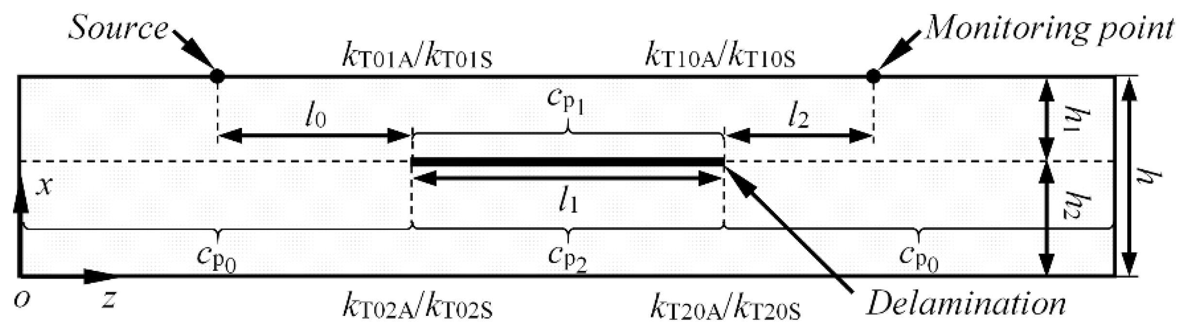
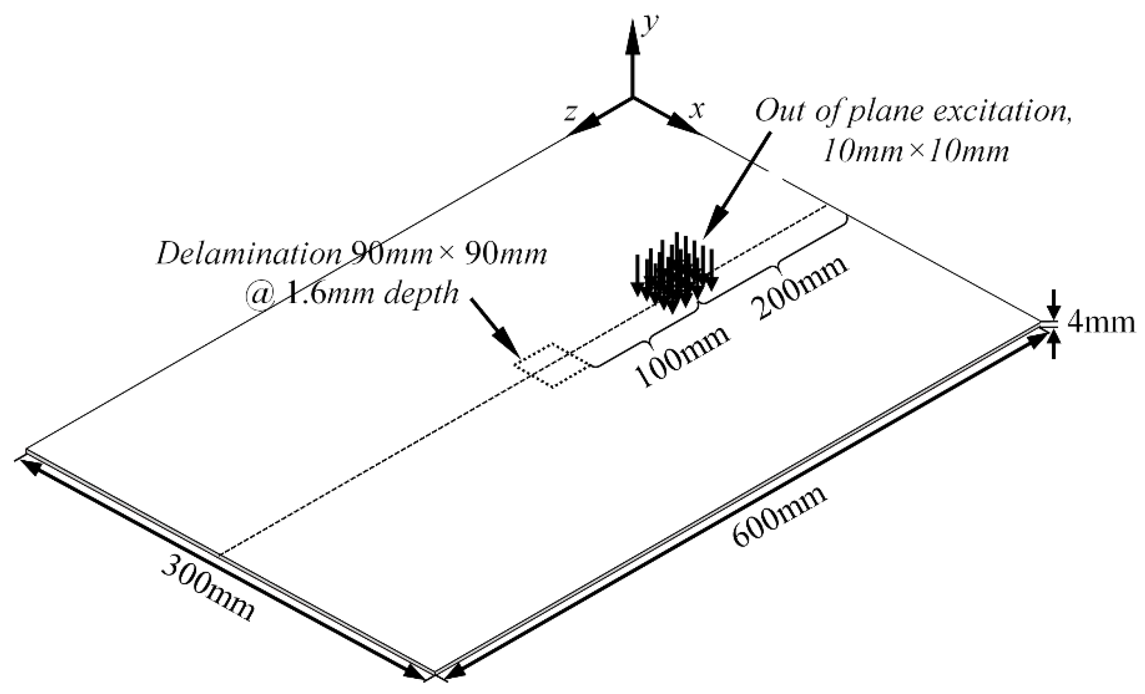
Let us analyze a composite plate with length l and thickness h which is shown in Figure 1. It will be investigated with the 2D approach, which means that the plate is infinite along the y axis. Let us consider that the delamination-type defect is present in the structure, which is l₁ long and situated at distances of l₀ and l₂ from the source (excitation) and monitoring (reception) points, respectively, at a depth of h₁ with respect to the top surface. The delamination is parallel to the surface of the sample (Figure 1).

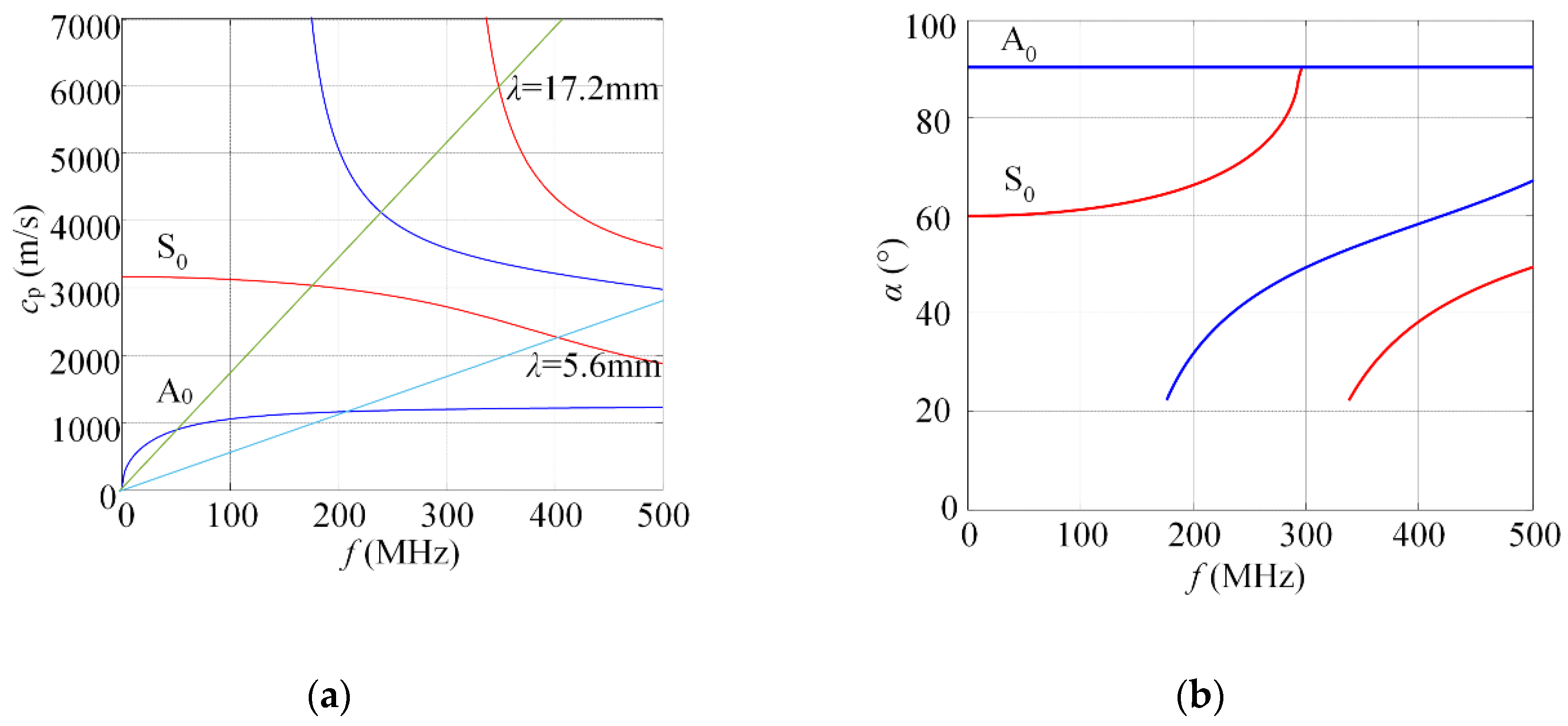
The fundamental A₀ mode has been selected in this paper. As multiple guided wave modes are being generated simultaneously, different strategies exist to excite isolated modes, such as angle beam excitation [27], element width selection [28], inter-element spacing or interdigital transducers [29,30], in-phase and out-of-phase excitation [31], etc. In this research the fundamental dispersion zone has been selected and the excitation frequencies were limited from 50 kHz up to 200 kHz. At such frequencies, the wavelengths of A₀ mode varies from 17.2 mm (at 50 kHz), to 5.6 mm (at 200 kHz) at 4 mm GFRP plate (E_x = 10 GPa, E_z = 35.7 GPa; υ_xz = 0.325, υ_zx = 0.091, υ_yx = 0.35; G_xz = 2.8 GPa; ρ = 1800 kg/m³). This shows that both A₀, S₀ and higher order A₁ and S₁ modes can exist at such a constant wavelength (see Figure 2a). However, using a Plexiglas wedge (2700 m/s) as a coupling medium and normal incidence angles, the fundamental A₀ mode is being generated most effectively (see Figure 2b), and sophisticated mode isolation techniques were not applied.

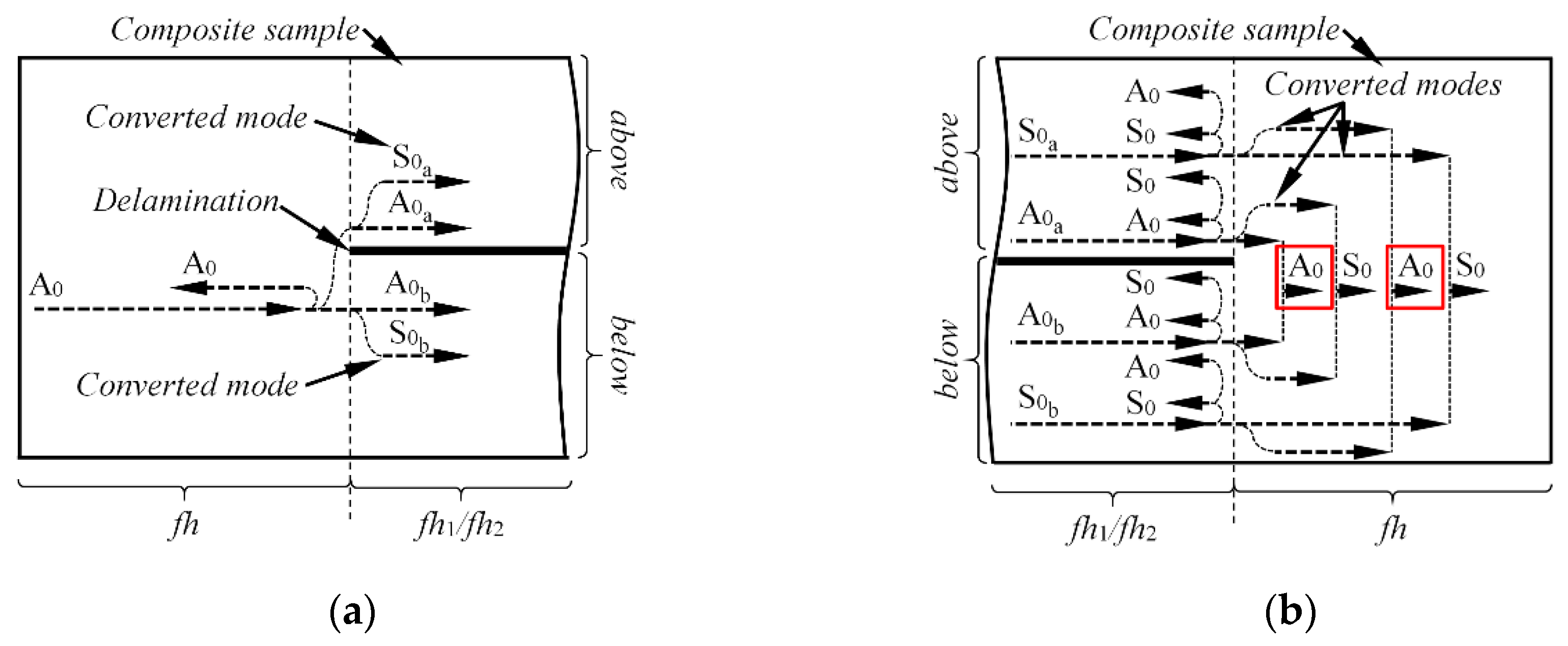
The signal of A₀ mode excited at the source point and measured at the monitoring point after propagation through the delaminated area will be the subject of all the upcoming investigations. Upon the interaction of A₀ mode with the delamination-type defect, the reflection, transmission and mode conversion occur at each end of the damage. In such a way, at the leading edge of the damage, the incident A₀ mode reflects back, and in the forward direction it splits into wave packets which accordingly propagate on the sub-laminates above and below the defect. Moreover, mode conversion occurs at the leading edge; therefore, part of the energy transforms into S₀ mode as well (see Figure 3a). Similarly, at the trailing edge of the damage, both A₀ and S₀ modes are reflecting back, propagating forward and converting to each other (see Figure 3b). This representation does not take into account the scattering coefficients of each reflected/converted mode.

In this research, only the forward scattered wave-packets of A₀ mode will be considered; they are squared red in Figure 3b. Mathematically, the spectrum of the signal of A₀ mode U_IA0(f) which arrives first to the monitoring (reception) point can be expressed as:

$$\begin{array}{cc}\hfill U_{{\mathrm{IA}}_0}\left(f\right)& =U_{{\mathrm{sA}}_0}\left(f\right)\cdot H\left(f,c_{p_0{A}_0},l_0\right)\cdot k_{\mathrm{T}01\mathrm{A}}\cdot H\left(f,c_{p_1{S}_0},l_1\right)\cdot k_{\mathrm{T}10\mathrm{S}}\cdot H\left(f,c_{p_0{A}_0},l_2\right)\\ & +U_{{\mathrm{sA}}_0}\left(f\right)\cdot H\left(f,c_{p_0{A}_0},l_0\right)\cdot k_{\mathrm{T}02\mathrm{A}}\cdot H\left(f,c_{p_2{S}_0},l_1\right)\cdot k_{\mathrm{T}20\mathrm{S}}\cdot H\left(f,c_{p_0{A}_0},l_2\right)\hfill \\ & =\left(U_{{\mathrm{sA}}_0}\left(f\right)\cdot H\left(f,c_{p_0{A}_0},L-l_1\right)\right)\cdot \left(\begin{array}{c}{k}_{\mathrm{T}01\mathrm{A}}\cdot H\left(f,c_{p_1{S}_0},l_1\right)\cdot k_{\mathrm{T}10\mathrm{S}}+\\ +k_{\mathrm{T}02\mathrm{A}}\cdot H\left(f,c_{p_2{S}_0},l_1\right)\cdot k_{\mathrm{T}20\mathrm{S}}\end{array}\right),\hfill \end{array}$$

(1)

$$H\left(f,c_{\mathrm{p}},l\right)=e^{-\alpha \left(f\right)x}{e}^{\frac{-jlf}{c_{\mathrm{p}}\left(f\right)}},$$

(2)

where U_sA0(f) is the frequency spectrum of the excitation signal of A₀ mode; H(f,c_p,l) is the transfer function of the waves propagating in the corresponding layer; c_pA0(f), c_pS0(f) are the phase velocities of A₀ and S₀ modes, respectively; l is the propagation distance (l₀, l₂–propagation distances in the defect-free area before and after the defect, respectively, l₁–length of the defect); L is the separation between the source and the monitoring points (L = l₀ + l₁ + l₂); and α(f) is the frequency dependent attenuation function; k_T01A, k_T02A, k_T10S and k_T20S are the transmission coefficients for A₀ and S₀ modes at the leading and trailing edges of the delamination, respectively, for the layer above and below the defect. The estimation of such reflection and transmission coefficients was out of the scope of this study. They essentially depend on the guided wave mode, the delamination depth, the material properties and the total thickness of the plate, and they should be determined for each particular case separately.

The wave packet described by Equation (1) is A₀ mode, which is a superposition of the signals traveling at upper and lower sub-laminates. This wave-packet converts from A₀ mode to S₀ mode at the leading edge and back to A₀ at the trailing edge of the defect. Due to this reason, this wave packet U_IA0(f) arrives earlier compared to the direct transmission of A₀ mode which does not convert within the defected area. This happens due to the reason that S₀ mode possesses a greater group velocity at low frequencies compared to A₀ mode. In this research, such a wave-packet shall be referred to as “first A₀ arrival”. Consequently, the frequency spectrum of the direct transmission of A₀ mode can be written as:

$$\begin{array}{c}{U}_{{\mathrm{IIA}}_0}\left(f\right)=U_{{\mathrm{sA}}_0}\left(f\right)\cdot H\left(f,c_{p_0{A}_0},l_0\right)\cdot k_{\mathrm{T}01\mathrm{A}}\cdot H\left(f,c_{p_1{A}_0},l_1\right)\cdot k_{\mathrm{T}10\mathrm{A}}\cdot H\left(f,c_{p_0{A}_0},l_2\right)\hfill \\ +U_{{\mathrm{sA}}_0}\left(f\right)\cdot H\left(f,c_{p_0{A}_0},l_0\right)\cdot k_{\mathrm{T}02\mathrm{A}}\cdot H\left(f,c_{p_2{A}_0},l_1\right)\cdot k_{\mathrm{T}20\mathrm{A}}\cdot H\left(f,c_{p_0{A}_0},l_2\right)\hfill \\ =\left(U_{{\mathrm{sA}}_0}\left(f\right)\cdot H\left(f,c_{p_0{A}_0},L-l_1\right)\right)\cdot \left(\begin{array}{c}{k}_{\mathrm{T}01\mathrm{A}}\cdot H\left(f,c_{p_1{A}_0},l_1\right)\cdot k_{\mathrm{T}10\mathrm{A}}+\\ +k_{\mathrm{T}02\mathrm{A}}\cdot H\left(f,c_{p_2{A}_0},l_1\right)\cdot k_{\mathrm{T}20\mathrm{A}}\end{array}\right).\hfill \end{array}$$

(3)

The “direct A₀ transmission” described by Equation (3) is the wave-packet which does not convert to other modes at the leading and trailing edges of delamination.

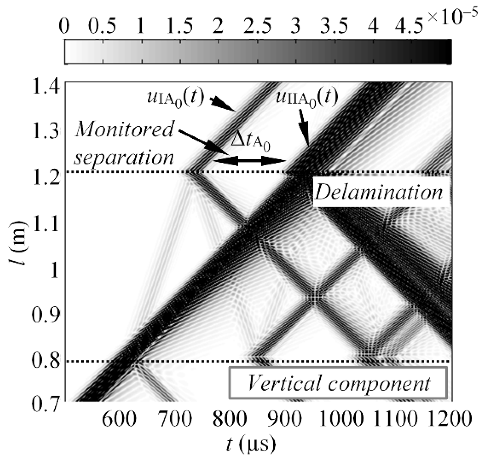
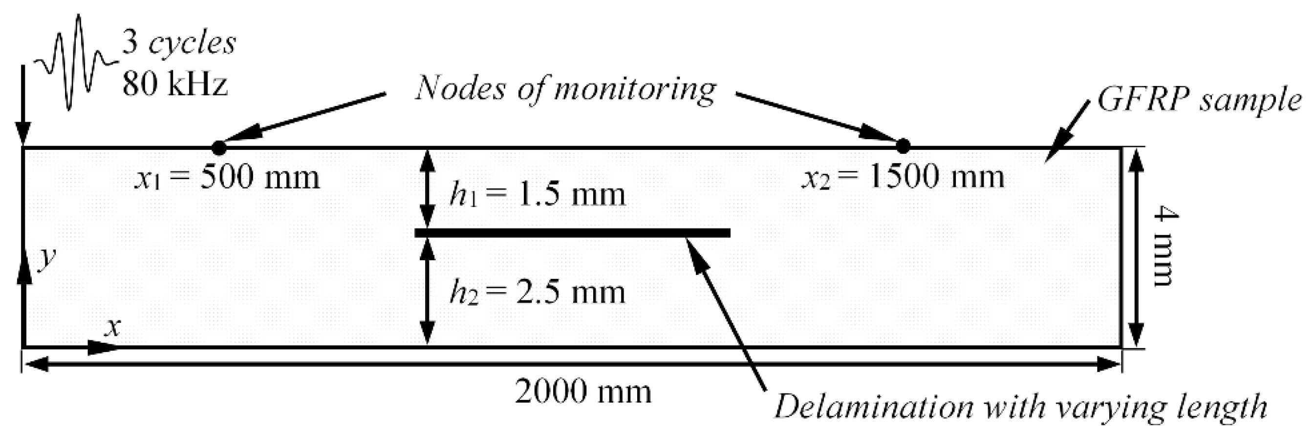
The scattering of the incident A₀ mode at the delamination-type defect is further illustrated with B-scans in Figure 4 which were simulated by using the Finite Element plane-strain model on a 2000 mm × 4 mm 2D GFRP plate. These B-scans represent a centered delamination-type defect located at a depth of 1.5 mm with respect to the top surface of the sample. A₀ mode was excited with a Gaussian envelope tone burst of three cycles and a central frequency of 80 kHz. The signals which are analyzed in this paper are denoted as u_IIA0(t) (“direct A₀ transmission”) and u_IA0(t) (“first A₀ arrival”) in Figure 4.

2.2. Method to Estimate the Depth of Defect

As it was shown by Equation (3), the “direct A₀ transmission” is a superposition of the waves traveling at the sub-laminates below and above the damage which does not convert to other modes, neither at the leading, nor at the trailing edge of the defect. If the delamination is asymmetrical across the thickness of the laminate (h₁ ≠ h₂ in Figure 1), the phase velocities at sub-laminates are different (c_p1 ≠ c_p2), and they depend on the excitation frequency and thickness of each sub-laminate. Beyond the defect, the modes from the upper and lower sub-laminates interfere with each other, which results in the single forward scattered A₀ mode u_IIA0(t). The magnitude of this mode is proportional to the result of interference which can be either in phase, out of phase or intermediate. If the transducer is driven by a set of different frequencies, a collection of magnitude variation patterns can be obtained and used for damage depth extraction. The use of multiple excitation frequencies enables one to exploit the frequency dependent phase velocity of A₀ mode, especially in the case of the presence of dispersion. Thus, the idea of the proposed method to estimate the depth of damage relies on the magnitude measurements of “direct A₀ transmission” u_IIA0(t) at burst signals with different central frequencies (f₁, f₂, … f_n). We should note that this technique is only valid if the delamination is asymmetrical h₁ ≠ h/2 ≠ h₂ and c_p1 ≠ c_p2. For ideally symmetrical delamination, there will be no out-of-phase interference of A₀ mode as the velocities at the layer above and below the defect will be very close.

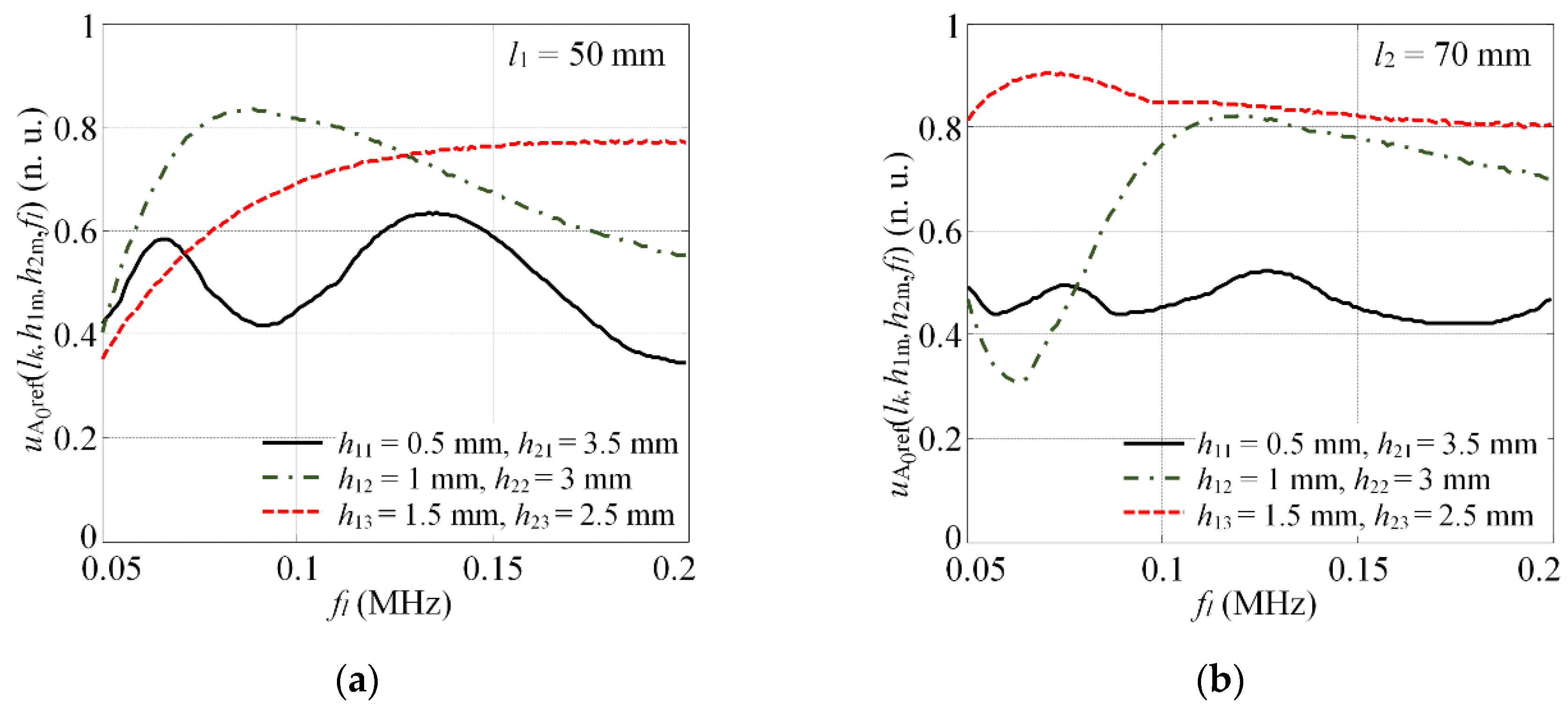
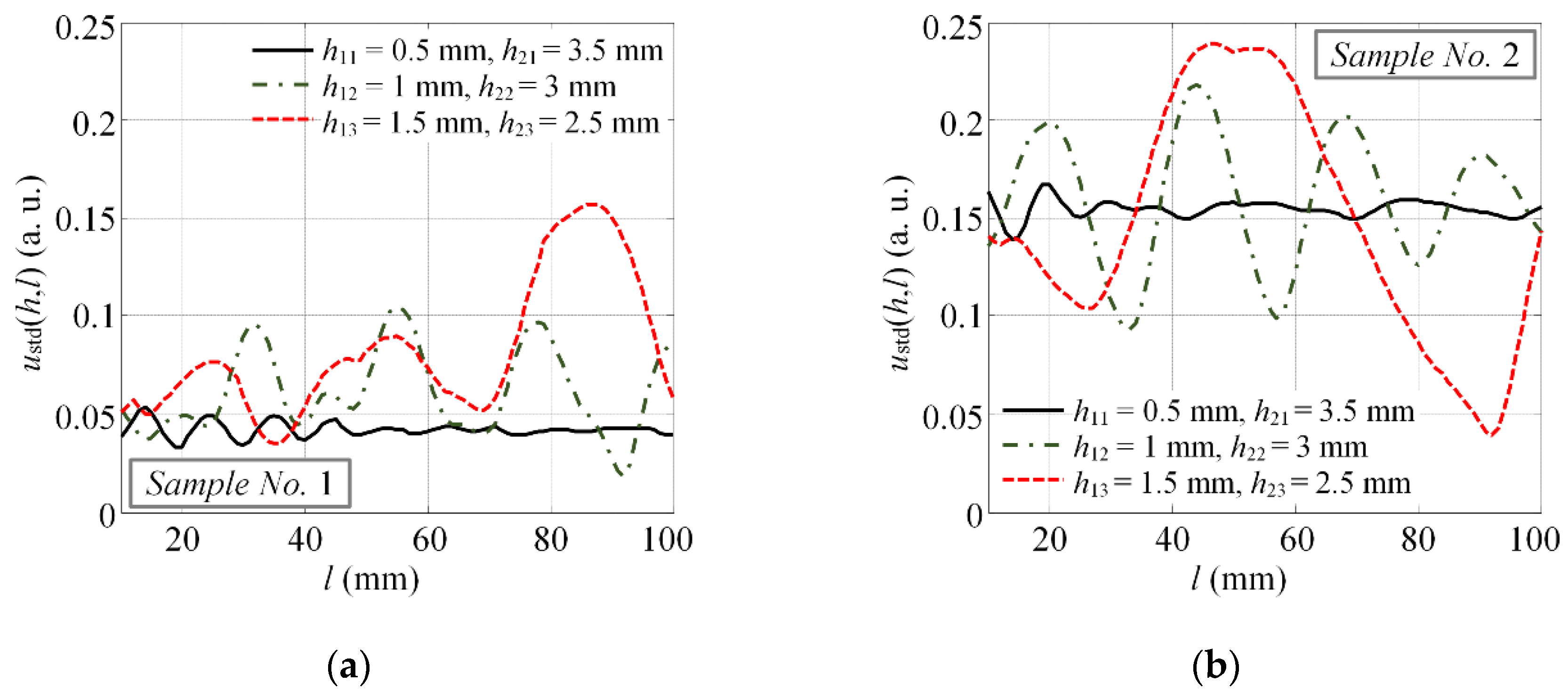
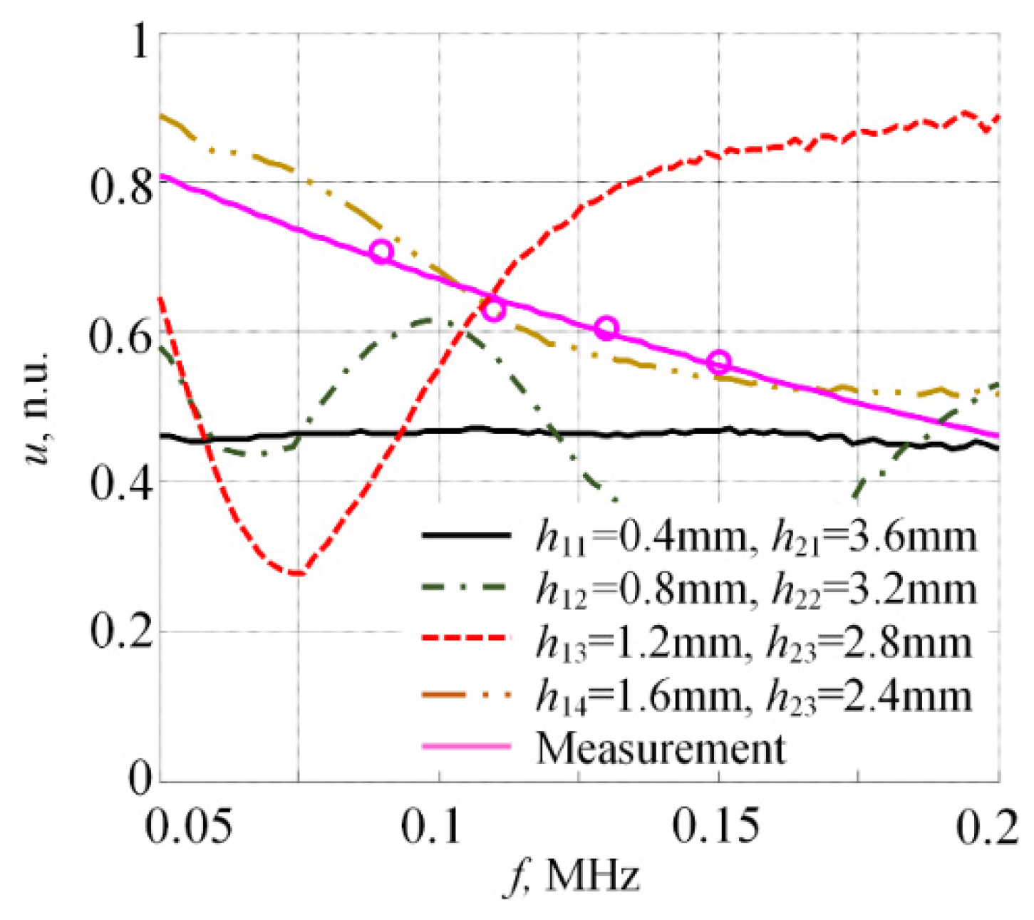
To extract the absolute values of the defect depth, a database of reference dependencies is required which would represent the collection of magnitude variation patterns at different excitation frequencies, the depth and the length of delaminations. Then, the estimated reference dependency can be compared to the experimental measurement in order to extract the depth of delamination. It is presumed that the reference dependency which best matches the experiments is the one that gives the closest definition of the damage depth in the structure. The step-by-step procedure of the damage depth estimation can be outlined as follows:

• The source of guided waves E is driven by burst with Gaussian envelope of central frequency f₁ to introduce A₀ mode in the investigated structure.
• Time trace u_A0(t) is received with sensor R_ref, which represents the structure without the damage (the reference signal). Meanwhile, the other receiver R₁ captures time history u_IIA0(t) which represents the response of the structure at the monitoring point beyond the defect.
• Ratio u_A0expf1(t) of peak-to-peak amplitudes of waveforms u_A0(t) and u_IIA0(t) is estimated at the burst central frequency f₁.
• Steps 1–3 are repeated over for other excitation frequencies f_N = (f₁, f₂, … f_n). As a consequence, the experimental dataset U_A0exp(f) = {f_N, u_A0expf1(t), u_A0expf2(t), …, u_A0expfn(t)} is collected, where f_N denotes the burst central frequencies used for the excitation of A₀ mode.
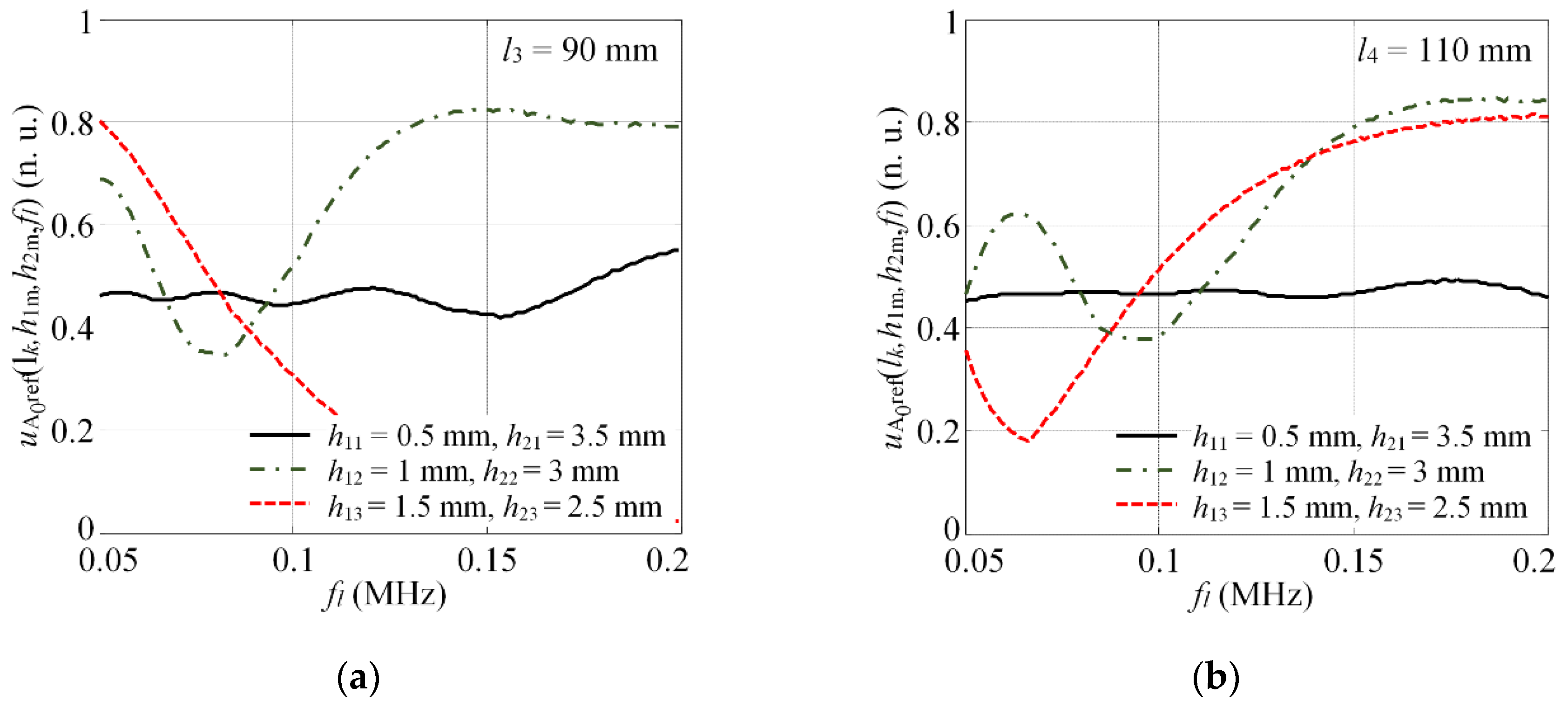
• The experimental dataset U_A0exp(f) is compared to the prescribed database of reference dependencies U_A0ref(f,h,l) (where h, l are the depth and the length of damage, respectively). Based upon this concept, the goal is to select the single reference dependency that is the closest to the experimental data. The criteria to characterize the similarity of two datasets include standard deviation as follows:

  $$h_{opt}=\underset{h}{\mathrm{argmin}}\left(\underset{l}{\mathrm{mean}}(u_{\mathrm{std}}\left(h,l\right))\right),$$

  (4)

  where

  $$u_{\mathrm{std}}\left(h,l\right)=\underset{f}{\mathrm{std}}\left(U_{A_0\mathrm{ref}}\left(f,h,l\right)-U_{A_0\exp }\left(f\right)\right),$$

  (5)

  where h_opt is the value which corresponds to the delamination depth where the reference dependency best matches the experimental dataset; U_A0ref(f,h,l) is the calculated reference dependency; U_A0exp(f) is the experimental dataset; h and l are the depth and the length of delamination, respectively; and “std” and “mean” denote the standard deviation and the arithmetic average, respectively.

If the structure is defect-free, function U_A0exp(f) is close to monotonic and does not feature essential amplitude variations. Meanwhile, if the variation in the magnitude ratio is observed, it can be related to the presence of a defect at a particular depth. The proposed depth estimation technique relies under the assumption, that velocities of direct A₀ mode in the upper and lower sub laminates are similar and the single wave packet is captured after the exit of delamination. In case of very large and asymmetric defects, two wave packets of A₀ mode can appear after the exit of the defect. In such a case, the inspection frequency must be decreased, or the number of signal cycles increased in order to maintain a single wave packet and to observe magnitude variation patterns.

2.3. Method to Assess the Length of Defect

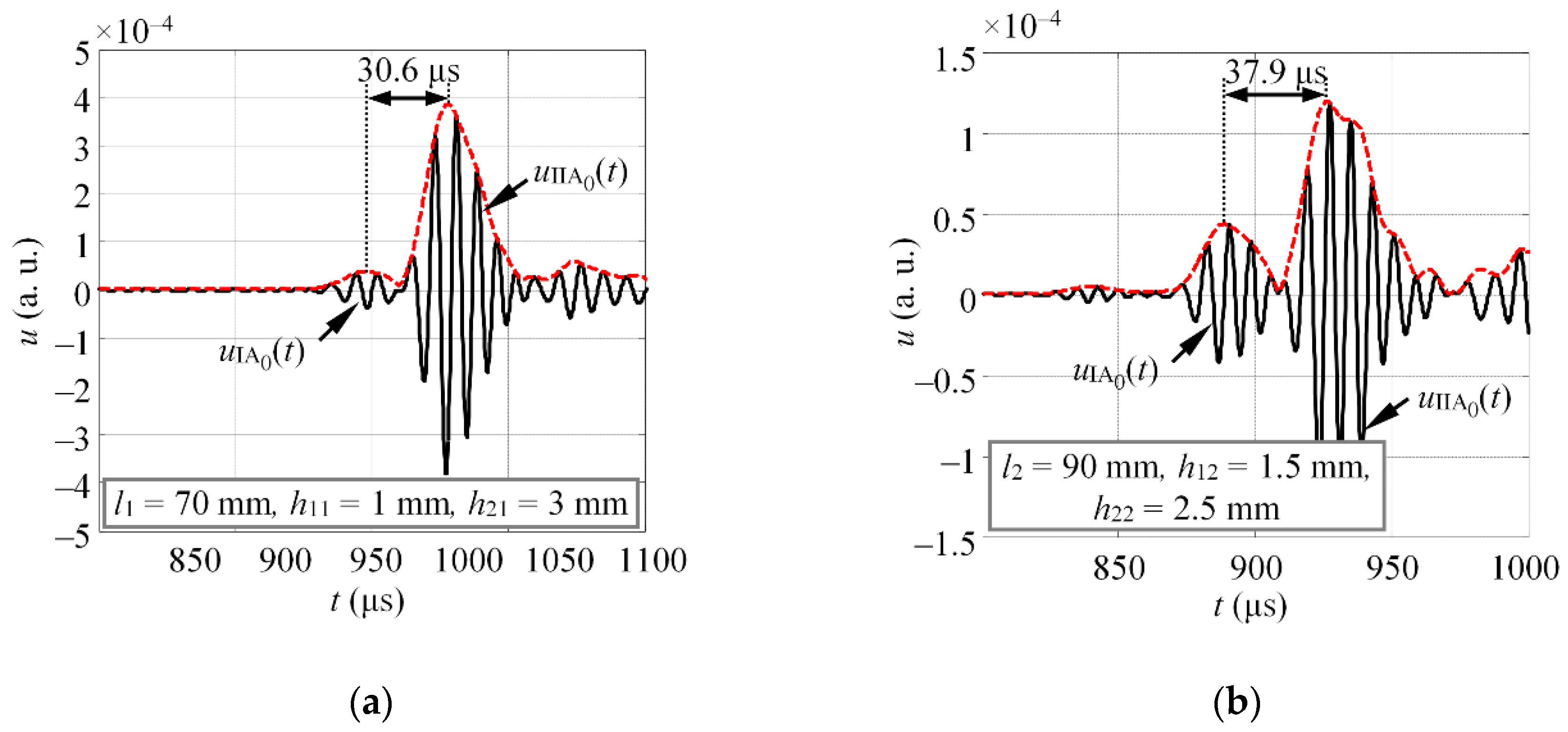
If the depth of the defect is determined, its length can be estimated from the delay between “direct A₀ transmission” u_IIA0(t) and “first A₀ arrival” u_IA0(t) which can be denoted as Δt_A0. Delay Δt_A0 is proportional to the excitation frequency and the propagation path of S₀ mode, which itself is actually determined by the length of the defect (Figure 5). The time delay between two neighboring wave packets can be estimated according to:

$$\mathsf{\Delta }{t}_{A_0}=\arg \underset{t}{\max }\left[\mathrm{HT}\left|u_{{\mathrm{IIA}}_0}\left(t\right)\right|\right]-\arg \underset{t}{\max }\left[\mathrm{HT}\left|u_{{\mathrm{IA}}_0}\left(t\right)\right|\right],$$

(6)

where u_IA0(t) and u_IIA0(t) are the wave packets of “first A₀ arrival” and “direct A₀ transmission”, and HT denotes the Hilbert transform. Then, the length of the defect at a particular depth h can be calculated as:

$$L_{\mathrm{def}}=\underset{f}{\mathrm{mean}}\left\{\mathsf{\Delta }{t}_{A_0}\left(h,f\right)·\frac{c_{{\mathrm{gA}}_0}\left(f\right)·c_{{\mathrm{gS}}_0}\left(f\right)}{c_{{\mathrm{gS}}_0}\left(f\right)-c_{{\mathrm{gA}}_0}\left(f\right)}\right\}.$$

(7)

The Equation (7) calculates mean defect length from a set of defect lengths obtained at different excitation frequencies. If multiple burst central frequencies are used to excite the guided waves, the group velocity values of A₀ and S₀ modes should be taken at different central frequencies, which allow one to consider the dispersion.

As the “direct A₀ transmission” u_IIA0(t) is the result of the interference between the wave packets propagating above and below the defect, the maximum of the wave after the exit of delamination (u_IIA0(t)) may be shifted and no longer correspond to the wave energy velocity. Hence the delay Δt_A0 in Equation (6) will be estimated with some error. The best way here would be to calculate the delay according to the mean energy (mass center) of the signal [32]. However, in such case the time window covering entire signal should be selected. Such a task is not trivial due to the dispersion of A₀ mode signals, presence of other modes and reflections from object boundaries. Additionally, the different frequency components of the dispersed A₀ mode are redistributed in the envelope of the signal. The lower frequency components are concentrated at the tail of the signal. So, the energy of wave packet u_IIA0(t) should be related to a particular frequency and velocity which are used for estimation of the time of flight. By using a maximum or Hilbert envelope of the signal it can be assumed that it corresponds to the dominant frequency of the signal and gives sufficient ToF accuracy.

It is noteworthy that, for the reliable operation of the method, direct u_IIA0(t) and converted modes u_IA0(t) must be separated in the time domain to an adequate extent in order to be able to measure the time delay between the two wave packets. Thus, there exists the minimum size of a defect that can be evaluated by using this approach. Such a minimum detectable defect is frequency dependent, so higher frequency signals can be used to improve sizing accuracy. It is important that the depth of the defect strongly influences the accuracy of the delamination length estimation, especially in the presence of significant dispersion. If the depth of the defect is unknown, such an approach becomes valid in non-dispersive regions only. However, by using the proposed delamination depth estimation technique, the thicknesses and velocities in the upper and lower sub-laminate can be determined, which leads to the improved accuracy of the delamination length evaluation.

3. Estimation of Reference Dependencies

As mentioned previously, the proposed technique to estimate the depth of delamination relies on reference calculations, which means that the experimental signals must be compared to the model-based predictions. In order to extract the depth of the damage, the dependencies between the magnitude of “direct A₀ transmission” U_A0ref(f,h,l), excitation frequency (f) and depth (h) at fixed defect lengths (l) will be calculated. In this study, for the sake of simplicity, the estimation of reference dependencies shall be demonstrated on the 2D model of a GFRP plate.

3.1. Theoretical Formulation of Reference Dataset

In the case of depth assessment, our goal is to predict the waveform of A₀ mode which propagates within the defect. Equation (3) can be rewritten in a short form as:

$$\begin{array}{c}{U}_{{\mathrm{IIA}}_0}\left(f\right)=\left(U_{{\mathrm{sA}}_0}\left(f\right)\cdot H\left(f,c_{p_0{A}_0},L-l_1\right)\right)\cdot \left(\begin{array}{c}{k}_{\mathrm{T}01\mathrm{A}}\cdot H\left(f,c_{p_1{A}_0},l_1\right)\cdot k_{\mathrm{T}10\mathrm{A}}+\\ +k_{\mathrm{T}02\mathrm{A}}\cdot H\left(f,c_{p_2{A}_0},l_1\right)\cdot k_{\mathrm{T}20\mathrm{A}}\end{array}\right)\hfill \\ =U_{A_0}\left(f\right)\cdot \left(U_{A_0\mathrm{ad}}\left(f\right)+U_{A_0\mathrm{bd}}\left(f\right)\right),\hfill \end{array}$$

(8)

where U_A0ad(f) and U_A0bd(f) represent the propagation of A₀ mode above and below the delamination, respectively. Waveforms u_A0ad(t) and u_A0bd(t) can be predicted according to the theory of linear acoustics which states that the output waveform of the system is the convolution of the input signal and the system impulse response. Consequently, each of the signals u_A0ad(t) and u_A0bd(t) can be expressed by the equations:

$$u_{A_0\mathrm{ad}}\left(t,l_k,h_{1m},f_l\right)=k_{\mathrm{T}01\mathrm{A}}\cdot k_{\mathrm{T}10\mathrm{A}}\cdot \mathrm{Re}\left\{{\mathrm{FT}}^{-1}\left\{\mathrm{FT}\left(u_{\mathrm{ref}}\left(t,f_l\right)\right)\cdot e^{-\alpha \left(f\right)l_k}{e}^{\frac{-j{l}_{k}f}{c_p\left(f{h}_{1m}\right)}}\right\}\right\},$$

(9)

$$u_{A_0\mathrm{bd}}\left(t,l_k,h_{2m},f_l\right)=k_{\mathrm{T}02\mathrm{A}}\cdot k_{\mathrm{T}20\mathrm{A}}\cdot \mathrm{Re}\left\{{\mathrm{FT}}^{-1}\left\{\mathrm{FT}\left(u_{\mathrm{ref}}\left(t,f_l\right)\right)\cdot e^{-\alpha \left(f\right)l_k}{e}^{\frac{-j{l}_{k}f}{c_p\left(f{h}_{2m}\right)}}\right\}\right\}$$

(10)

where u_ref(t, f_l) is the theoretical incident signal at a particular excitation frequency (l = 1 ÷ M, M is the total number of frequencies used to drive the emitter); α(f) is the attenuation function; l_k is the length of the defect (k = 1 ÷ N, where N is the total number of length incrementations); c_p(f,h_1m) and c_p(f,h_2m) are the phase velocities for the layer above (h_1m) and below the defect (h_2m) which depend on the level of defect asymmetry; h_1m and h_2m are the thicknesses of the layer above and below the defect; and FT denotes the Fourier transform. The in phase or out of phase interference of these signals defines the peak to peak amplitude of “direct A₀ transmission” u_A0ref(l_k,h_1m,h_2m,f_l) at excitation frequency f_l:

$$\begin{array}{c}{u}_{A_0\mathrm{ref}}\left(l_k,h_{1m},h_{2m},f_l\right)=\underset{t}{\max }\left(u_{A_0\mathrm{ad}}\left(t,l_k,h_{1m},f_l\right)+u_{A_0\mathrm{bd}}\left(t,l_k,h_{2m},f_l\right)\right)\hfill \\ -\underset{t}{\min }\left(u_{A_0\mathrm{ad}}\left(t,l_k,h_{1m},f_l\right)+u_{A_0\mathrm{bd}}\left(t,l_k,h_{2m},f_l\right)\right).\hfill \end{array}$$

(11)

To illustrate the estimation of reference dependency, let us consider a GFRP plate of thickness h = 4 mm with delamination-type defects situated at various depths as follows: h_1m = mh/8, h_2m = h − h_1m, where m = 1, 2,…,3. Let us assume that the excitation burst central frequency of the incident A₀ mode varies starting from 50 kHz to 200 kHz with increments of 1 kHz. The graphic illustration of the magnitude of A₀ mode u_A0ref(l_k,h_1m, h_2m,f_l) as the function of excitation frequency f_l at discrete depths h_1m = mh/8, h_2m = −h_1m is illustrated in Figure 6 and Figure 7. The results are presented at fixed defect lengths of l₁ = 50 mm, l₂ = 70 mm, l₃ = 90 mm and l₄ = 110 mm. Each graph in Figure 6 and Figure 7 represent magnitude variation of forward scattered A₀ mode at different excitation frequencies. It can be observed that the magnitude variation of “direct A₀ transmission” depends not only on the depth of the defect (which is represented by solid, dashed and dash-dot lines) but on its length as well. As one might expect, the size of the defect could be estimated from the same magnitude variations. However, these magnitude variations due to the length of the defect repeat. For example, if the defect is 0.5 mm below the surface (solid line), the magnitude variation versus frequency is almost identical at defect lengths of l₃ = 90 mm (Figure 7a) and l₄ = 110 mm (Figure 7b). It means that multiple defect lengths correspond to the same magnitude variation of A₀ mode. On the other hand, the observed magnitude variations due to the depth are always different. Therefore, in this paper it is suggested to use magnitude variation for damage depth estimation only and then apply time of flight measurement techniques to estimate the size of defect. By knowing the depth of the damage, the accuracy of damage sizing can be increased, as the actual depth of defect determines the phase velocities of A₀ and S₀ modes in the upper and lower sub-laminates.

3.2. Numerical and Experimental Verification of Reference Dependencies

In the following chapter, the reference dependency estimation technique presented in the previous section is verified with the appropriate numerical simulations and experiments on GFRP and aluminum samples. To achieve the aim of this study, the numerically and experimentally estimated amplitude variations in the case of different lengths of a defect are compared with the predictions calculated by Equation (11). It is important to distinguish that in this verification, magnitude variations of forward scattered A₀ mode are being estimated at different lengths of defect as it was impossible to iteratively change the depth of defect in experiments. The proposed damage detection technique itself uses magnitude variation for damage depth assessment, while the length is extracted from time of flight (ToF) measurements.

3.2.1. Numerical Verification

At first, the reference dependency estimation technique is verified numerically. A total number of 50 2D linear structural mechanics FE models were employed for an anisotropic GFRP plate with the dimensions of x = 2000 mm, y = 4 mm. In this case, the plain strain model was implemented by assuming that the object is infinite in the z direction. In each of the 50 models, delamination-type defects were introduced 1.5 mm below the surface (h₁ = 1.5 mm, h₂ = 2.5 mm) by separating the appropriate nodes of the mesh. The length of delamination l varied from 10 to 500 mm with an increment of 10 mm, thus yielding a total number of 50 numerical models. The delamination was centered horizontally along the x axis of the investigated sample for all the defect lengths. Throughout the simulations, 2D structural solid plane-42 finite elements were used. The spatial size of the element was equal to 0.5 mm, which corresponds to 26 nodes per wavelength if the slowest A₀ mode at 80 kHz central frequency is considered. The excitation signal in all cases was a Gaussian envelope tone burst of three cycles and a central frequency of 80 kHz. Such an excitation regime was deliberately selected to converge with the experimental verification, which will be described further in this section. A₀ mode was introduced by applying out-of-plane displacements to the first node column of the model located on the sample edge (see Figure 8). Such a force excites both fundamental A₀ and S₀ modes at a given frequency band and acts similarly to a simple thickness mode transducer. The integration step in the time domain was 0.625 µs, which is 1/20 of the period at 80 kHz central frequency. Throughout the simulation, a generalized stiffness matrix was used to describe a symmetric GFRP laminate (biaxial: 0° and 90°/bias: ±45°/biaxial: 0° and 90°)_S, while employing the research conducted by Ryan et al. [33] Hence, the stiffness matrix was obtained by summing up the contribution of each ply in terms of their respective thicknesses. The following material properties of GFRP were used: Young’s modulus (E_x = 10 GPa, E_z = 35.7 GPa); Poisson’s ratio (υ_xz = 0.325, υ_zx = 0.091, υ_yx = 0.35); shear modulus G_xz = 2.8 GPa; density ρ = 1800 kg/m³. The sketch of the numerical model used in this study is presented in Figure 8.

The variable monitored in this study was the vertical component of particle velocity (y) at the nodal locations before (x₁ = 500 mm, y₁ = 4 mm) and beyond (x₂ = 1500 mm, y₂ = 4 mm) the defect (see Figure 8). The obtained peak to peak amplitude variations versus the length of delamination are presented in Figure 9. In the same figure, the predicted curve obtained by using Equation (11) with identical parameters is presented as the solid line.

3.2.2. Experimental Verification

In addition to numerical calculations, experiments on a custom-made aluminum alloy plate with the dimensions of 1250 mm × 600 mm × 5 mm were carried out as well. The aluminum plate was selected for the verification of the method due to a few reasons. At first, the properties of aluminum and the dispersion relations of guided waves in it are well known. The second reason is that it was the most reliable way to create thin delamination with a strictly defined length. Afterwards, the method can be applied on any other types of materials with known properties. In the experiments, a special aluminum sample with a machined groove was produced in order to obtain the response adequate to that obtained with the delamination-type defect. In the course of the production of the sample, two aluminum sheets with thicknesses of 2 mm and 3 mm were bonded adhesively to produce a total thickness of 5 mm. Prior to bonding, the 3 mm sheet was machined to produce a wedge-shaped groove with a depth of 500 µm. The lateral dimensions of the groove ranged from 35 to 335 mm, which enabled the delamination-type defect of a variable size to be simulated. The sketch of the experimental setup used for validation purposes is presented in Figure 10a.

The experimental investigation was conducted by using custom-made low frequency ultrasonic transducers (130 kHz) operating in a thickness mode with an active diameter of 10 mm. The transducers possess the bandwidth of 100 kHz at −6 dB level and were driven by a 50 V tone-burst with a Gaussian envelope of 3 periods and a central frequency of 130 kHz. The number of cycles were selected to maintain a good balance between the amplitude measurements for depth estimation which requires narrowband excitation and ToF measurements for defect length assessment where a wideband excitation is preferred for better resolution. The best compromise between the propagation distance, the number of cycles, the wavelength and the resolution was selected according to the concept of the minimum resolvable distance (MRD), which was described by Wilcox et al. [34] In the experiment, the transducers were arranged in a pitch–catch configuration and attached perpendicularly to the surface of the sample to introduce A₀ mode. The transmitter and the receiver were linked together and scanned along the short edge of the artificial defect as it is shown in Figure 10a. To achieve a reliable and uniform acoustic contact between the transducer and the specimen, custom-made spring type adjusters were used (Figure 10b). As a result of the experiment, a set of waveforms at different defect lengths were collected. The peak-to-peak amplitude of each time trace was compared to the reference time history captured at the same basis on the defect-free region.

The comparison between mathematical predictions and experimental measurements can be seen in Figure 11. The results demonstrate a fairly good agreement between the experimental values and the mathematical predictions, especially below the defect lengths of 200 mm. The mismatch in the amplitude ratio between the mathematical and experimental estimations may appear due to the mismatch of dispersion curves, ignored transmission and reflection coefficients in Equations (9) and (10), and by diffraction losses. The discrepancies between magnitude variations and length of defect that are visible in Figure 9 and Figure 11 have a minor impact for damage depth estimation. The actual size of the defect is obtained from ToF measurement, using the damage depth information from magnitude variation of forward scattered direct A₀ mode.

4. Verification of Proposed Delamination Depth and Length Estimation Technique

4.1. Verification with 2D Model

To demonstrate the overall performance of the proposed delamination depth and length estimation method, two separate 2D GFRP finite element models, both with dimensions of 2000 mm × 4 mm shall be considered. For the sake of better understanding, let us denote them as sample No. 1 and sample No. 2. Each of the considered models contains delaminations of different sizes and through-thickness locations. In sample No. 1, the delamination with a length of x₁ = 70 mm is introduced 1 mm below the top surface (h₁₁ = 1 mm, h₂₁ = 3 mm). Meanwhile, sample No. 2 has a defect of x₂ = 90 mm located at a depth of 1.5 mm (h₁₂ = 1.5 mm, h₂₂ = 2.5 mm). A sketch of the considered cases is presented in Figure 12.

Throughout the simulations, 2D structural solid plane-42 finite elements were used. The same properties of GFRP laminate were maintained as described in the previous section. In each of the investigated cases, a Gaussian envelope tone burst of three cycles was used for excitation. The excitation frequencies were changed within the range from f₁ = 50 kHz to f_n = 200 kHz with increments of 10 kHz. Hence, 16 different excitation frequencies were used for each of the two considered models. The spatial size of the element in all cases was constant and equal to 0.5 mm, which corresponds to 12 up to 37 nodes per wavelength for the slowest A₀ in a frequency range of f₁, f₂, …, f_n. A₀ mode was introduced into the structure by applying the out-of-plane nodal displacements to the edge of the sample in the same way as it was demonstrated in Figure 8. The integration step in the time domain varied from 1 µs for the lowest excitation frequency f₁ = 50 kHz to 0.25 µs for f_n = 200 kHz. The variable monitored in this study was a vertical component of the particle velocity (y) at nodal locations r₁ (x₁ = 750 mm, y₁ = 4 mm) and r₂ (x₂ = 1250 mm, y₂ = 4 mm).

4.1.1. Estimation of Defect Depth

In order to estimate the depth of the defect, the procedure described in Section 2 is employed. The reference dependency is calculated according to Equations (9)–(11) for defect lengths l₁ = 10 mm, l₂ = 11 mm, …, l_N = 100 mm and defect depths h₁₁ = 0.5 mm, h₁₂ = 1 mm and h₁₃ = 1.5 mm for the same set of excitation frequencies (f₁ = 50 kHz, f₂ = 60 kHz, …, f_n = 200 kHz). Then, h_opt is calculated by using Equation (4) in order to estimate the depth of the damage. The graphic illustration of u_std(h,l) at different lengths and depths is presented in Figure 13. The criteria to estimate the actual depth of the defect are based on the selection of the minimum of u_std(h,l). The estimated h_opt values for sample No. 1 and sample No. 2 at different depths of the defect are summarized in

Table 1. h_opt values for sample No. 1 and sample No. 2 which are used as a criterion to estimate the depth of delamination.

	Sample No. 1	Sample No. 2
	hopt	hopt
h11 = 0.5 mm, h21 = 3.5 mm	0.033	0.137
h12 = 1 mm, h22 = 3 mm	0.018	0.091
h13 = 1.5 mm, h23 = 2.5 mm	0.035	0.036

.

It can be observed that, for sample No. 1 (Figure 13a), h_opt is close to zero for depth h₁₂ = 1 mm (the dash-dot line in Figure 13a). Hence, the estimated depth of delamination for sample No. 1 is 1 mm, which corresponds to the actual depth of the damage. Similar observations may be made for sample No. 2. h_opt possesses the lowest values at depth h₁₃ = 1.5 mm (the dashed line in Figure 12b), which is in agreement with the actual depth of the damage. In the presented case, the actual depth of the damage was included in the database. In order to evaluate the performance of the method in case of absence of actual depth in database, another set of magnitude patterns has been generated with depth increments of 0.4 mm (h₁₁ = 0.4 mm, h₁₂ = 0.8 mm, h₁₃ = 1.2 mm, h₁₄ = 1.6 mm, h₁₅ = 2 mm). In the case for sample No. 1 the minimum values of the h_opt were close for both h₁₂ = 0.8 mm and h₁₃ = 1.2 mm, however the absolute minimum was obtained for depth h₁₂ = 0.8 mm. For sample No. 2 h_opt possesses the lowest values at depth h₁₄ = 1.6 mm. The amount of error of course depends on the depth increments in the database. Such database in general is computationally inexpensive (in this case U_A0ref(11 × 5 × 90), hence can be calculated small depth increments according to the desired depth estimation accuracy.

4.1.2. Evaluation of Defect Length

As the depth of the defect for both samples has been determined, the length is estimated by measuring the delay between the “first A₀ arrival” u_IA0(t) and “direct A₀ transmission” u_IIA0(t) of A₀ mode. The delays are measured according to the maximum envelope values of each wave packet by using Equation (6). Then, the length of the defect is estimated according to Equation (7).

In this particular case, the delay values are estimated at a single excitation frequency f₉ = 130 kHz. The vertical component of the particle velocity at nodal point r₂ for sample No. 1 and sample No. 2 is presented in Figure 14a,b. The picture shows the wave packets of “first A₀ arrival” u_IA0(t) and “direct A₀ transmission” u_IIA0(t), along with the estimated delay values according to the Hilbert envelope.

According to Equation (7), the delay time values correspond to the defect length of 67.6 mm for sample No. 1, meanwhile, for sample No. 2, the delay indicates the length of 83.4 mm. The results demonstrate that the average error in the length estimation is approximately 6% relative to the actual size. Such error is valid for frequency range between 50 and 200 kHz for defect sizes of 70 mm and 90 mm. The amount of error depends both on the accuracy of damage depth estimation and the delay time measurement. For different defect sizes and excitation frequencies, the errors may change. However, the accuracy of defect size and depth estimation can still be improved by adding scattering coefficients to the reference model and measuring delay time according to the mass center of the signal instead of using Hilbert envelope.

4.2. Verification with 3D Model

In order to verify the applicability of the method for the real measurement, the 3D case was investigated. The reason for that is that in the case of 2D modeling of guided waves, the diffraction does not affect the signals, in contrary to the 3D case when diffraction takes place, and signals can be overlapped with boundary reflections. There are many signal processing methods which work perfectly in the case of 1D or 2D models; however, they still fail when they are applied for real structures or 3D models. So, the verification of the method for a 3D case is very important for the assessment of the potential of the method for in situ applications.

For this purpose, a 3D GFRP numerical model with the dimensions of 600 mm × 300 mm × 4 mm was employed with a square (90 mm × 90 mm) delamination-type defect, located at 1.6 mm below the top surface. The defect was centered both according to the x and z axes (Figure 15). The structure was meshed by using SOLID64 elements which had eight nodes each with three degrees of freedom. The properties of the GFRP structure were the same as it was described in the previous sections. The spatial size of the element was set to 0.8 mm, which corresponds to 16 nodes per wavelength for A₀ mode at 90 kHz central frequency. In total, four 3D models were created, each with a different excitation frequency which was varying from 90 kHz to 150 kHz with an increment of 20 kHz. The excitation zone was a square with dimensions of 10 mm by 10 mm. It was centered according to the x axis and had an offset of 200 mm from the origin of the z axis. The excitation signal in all the cases was a Gaussian envelope tone burst of three cycles in order to correspond to the previous experiments. A₀ mode was introduced by applying the normal out-of-plane nodal displacements to the top surface of the sample at a predefined area of 10 mm². The integration step in the time domain was 0.625 µs, which is 1/18 of the period at 90 kHz central frequency. The sketch of the numerical model used in this study is presented in Figure 15.

The magnitude variation of A₀ mode was estimated at various excitation frequencies (f₁ = 90 kHz, f₂ = 110 kHz, f₃ = 130 kHz, f₄ = 150 kHz) and compared to the database of predictions at different defect depths (h₁₁ = 0.4 mm, h₁₂ = 0.8 mm, h₁₃ = 1.2 mm, h₁₄ = 1.6 mm) and lengths (l₁, l₂, … l_n). The comparison between the measured magnitude variation from the 3D model and the prediction at the defect size of 90 mm is presented in Figure 16. As it can be observed, the approximated curve which goes through the measured magnitude values (the solid line) is close to the prediction at depth h₁₄ (the dash double-dot line). This depth of the damage corresponds to the actual depth used in the model. To measure the match between the measurement and the reference dependency, the parameter h_opt described by Equation (4) was used. The results are summarized in

Table 2. h_opt values used as a criterion to estimate the depth of delamination in 3D model.

	h11 = 0.4 mm, h21 = 3.6 mm	h12 = 0.8 mm, h22 = 3.2 mm	h13 = 1.2 mm, h23 = 2.8 mm	h14 = 1.4 mm, h24 = 2.6 mm
hopt	0.068	0.034	0.023	0.019

.

The results presented in Table 2 show that the correct damage depth estimation was observed by using the parameter h_opt. For the damage length estimation, the delay between direct and converted A₀ modes was estimated at a frequency of f₄ = 150 kHz. The measured delay was equal to Δt_A0 = 38.1 μs. It was compared to the estimated delay at a defect depth of h₁₄ = 1.4 mm. It can be observed that the estimated delay values correspond to the defect length of 84.1 mm. In this case, the length estimation error is approximately 6.5% relative to the actual size of the defect. We should note that, in the 3D case, the size of the defect is evaluated in the direction of wave propagation only.

5. Conclusions

A model-based method to estimate the absolute depth and length of delamination was proposed which is based on the magnitude variation pattern and the time-of-flight measurement of A₀ mode at different excitation frequencies.

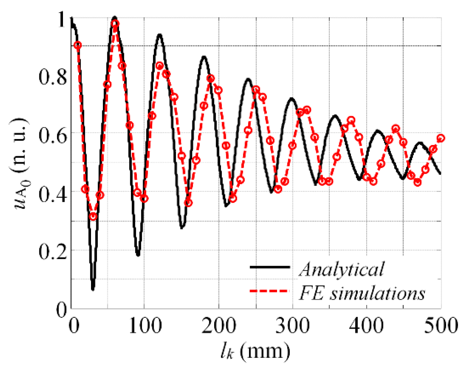
A reference dependency estimation technique was developed which allows predicting the magnitude variation patterns of A₀ mode at different depths and lengths of a delamination-type defect. It was shown that, in comparison with the experimental measurements, the reference dependencies can be used to extract the absolute depth of the delamination. The proposed delamination depth estimation technique exploits the phase velocity dependency of A₀ mode on the thickness of the sub-laminate, thus, different magnitude variation patterns at different excitation frequencies are observed. As a result, the proposed method provides improved depth estimation accuracy even in the presence of significant dispersion. Furthermore, finite element verification demonstrated that the defect depth can be estimated with a high accuracy even in those cases when the thickness of the sub-laminate that is created by the presence of the defect is relatively thin in comparison with the wavelength of A₀ mode. The performance of the proposed method was demonstrated and verified in detecting and describing delamination-type defects of various lengths and depths.

It was demonstrated that the length of delamination at a fixed depth can be reliably estimated from the delay time between the converted and direct A₀ modes by exploiting the conversion of the incident A₀ mode to S₀ mode within the defect. The proposed approach uses previously obtained information about the depth of the defect, which allows for the determination of the phase velocities of A₀ and S₀ modes in the upper and lower sub-laminates. The results of our numerical validation demonstrated that the size of the defect can be reconstructed with an error of approximately 6%.

The main value of the proposed technique lies in multi-frequency excitation, which leads to different magnitude patterns of A₀ mode for delamination depth assessment and more accurate velocity values for defect length estimation. Hence, such a technique can be used even in the presence of the dispersion of A₀ mode and provide information about the absolute depth and length of the damage by employing a few time traces measured at slightly different frequencies.

References

1. Ip, K.; Mai, Y. Delamination Detection in Smart Composite Beams using Lamb Waves. Smart Mater. Struct. 2004, 13, 544–551. [Google Scholar] [CrossRef]
2. Shoja, S.; Berbyuk, V.; Boström, A. Delamination Detection in Composite Laminates using Low Frequency Guided Waves: Numerical Simulations. Compos. Struct. 2018, 203, 826–834. [Google Scholar] [CrossRef]
3. Ramadas, C.; Balasubramaniam, K.; Joshi, M.; Krishnamurthy, C.V. Characterisation of Rectangular Type Delaminations in Composite Laminates through B- and D-Scan Images Generated using Lamb Waves. NDT E Int. 2011, 44, 281–289. [Google Scholar] [CrossRef]
4. Santos, M.; Perdigão, J. Leaky Lamb Waves for the Detection and Sizing of Defects in Bonded Aluminium Lap Joints. NDT E Int. 2005, 38, 561–568. [Google Scholar] [CrossRef]
5. Sohn, H.; Dutta, D.; Yang, J.Y.; Park, H.J.; DeSimio, M.; Olson, S.; Swenson, E. Delamination Detection in Composites through Guided Wave Field Image Processing. Compos. Sci. Technol. 2011, 71, 1250–1256. [Google Scholar] [CrossRef]
6. Zhao, G.; Wang, B.; Wang, T.; Hao, W.; Luo, Y. Detection and Monitoring of Delamination in Composite Laminates using Ultrasonic Guided Wave. Compos. Struct. 2019, 225, 111161. [Google Scholar] [CrossRef]
7. Panda, R.S.; Rajagopal, P.; Balasubramaniam, K. Characterization of Delamination-Type Damages in Composite Laminates using Guided Wave Visualization and Air-Coupled Ultrasound. Struct. Health Monit. 2017, 16, 142–152. [Google Scholar] [CrossRef]
8. Feng, B.; Ribeiro, A.L.; Ramos, H.G. Interaction of Lamb Waves with the Edges of a Delamination in CFRP Composites and a Reference-Free Localization Method for Delamination. Measurement 2018, 122, 424–431. [Google Scholar] [CrossRef]
9. Hayashi, T.; Kawashima, K. Multiple Reflections of Lamb Waves at a Delamination. Ultrasonics 2002, 40, 193–197. [Google Scholar] [CrossRef]
10. Guo, N.; Cawley, P. The Interaction of Lamb Waves with Delaminations in Composite Laminates. J. Acoust. Soc. Am. 1993, 94, 2240–2246. [Google Scholar] [CrossRef]
11. Li, F.; Peng, H.; Sun, X.; Wang, J.; Meng, G. Wave Propagation Analysis in Composite Laminates Containing a Delamination using a Three-Dimensional Spectral Element Method. Math. Probl. Eng. 2012, 2012. [Google Scholar] [CrossRef]
12. Ramadas, C.; Balasubramaniam, K.; Joshi, M.; Krishnamurthy, C.V. Interaction of the Primary Anti-Symmetric Lamb Mode (Ao) with Symmetric Delaminations: Numerical and Experimental Studies. Smart Mater. Struct. 2009, 18, 085011. [Google Scholar] [CrossRef]
13. Ramadas, C.; Balasubramaniam, K.; Joshi, M.; Krishnamurthy, C.V. Interaction of Guided Lamb Waves with an Asymmetrically Located Delamination in a Laminated Composite Plate. Smart Mater. Struct. 2010, 19, 065009. [Google Scholar] [CrossRef]
14. Ramadas, C.; Janardhan Padiyar, M.; Balasubramaniam, K.; Joshi, M.; Krishnamurthy, C.V. Delamination Size Detection using Time of Flight of Anti-Symmetric (Ao) and Mode Converted Ao Mode of Guided Lamb Waves. J. Intell. Mater. Syst. Struct. 2010, 21, 817–825. [Google Scholar] [CrossRef]
15. Schaal, C.; Zhang, S.; Samajder, H.; Mal, A. An Analytical Study of the Scattering of Ultrasonic Guided Waves at a Delamination-Like Discontinuity in a Plate. Proc. Inst. Mech. Eng. Part C 2017, 231, 2947–2960. [Google Scholar] [CrossRef]
16. Hu, N.; Shimomukai, T.; Yan, C.; Fukunaga, H. Identification of Delamination Position in Cross-Ply Laminated Composite Beams using S0 Lamb Mode. Compos. Sci. Technol. 2008, 68, 1548–1554. [Google Scholar] [CrossRef] [Green Version]
17. Shkerdin, G.; Glorieux, C. Lamb Mode Conversion in a Plate with a Delamination. J. Acoust. Soc. Am. 2004, 116, 2089–2100. [Google Scholar] [CrossRef]
18. Birt, E.A. Damage Detection in Carbon-Fibre Composites using Ultrasonic Lamb Waves. Insight 1998, 40, 335. [Google Scholar]
19. Liu, Z.; Yu, H.; He, C.; Wu, B. Delamination Detection in Composite Beams using Pure Lamb Mode Generated by Air-Coupled Ultrasonic Transducer. J. Intell. Mater. Syst. Struct. 2014, 25, 541–550. [Google Scholar] [CrossRef]
20. Li, B.; Ye, L.; Li, Z.; Ma, Z.; Kalhori, H. Quantitative Identification of Delamination at Different Interfaces using Guided Wave Signals in Composite Laminates. J. Reinf. Plast. Compos. 2015, 34, 1506–1525. [Google Scholar] [CrossRef]
21. Petculescu, G.; Krishnaswamy, S.; Achenbach, J.D. Group Delay Measurements using Modally Selective Lamb Wave Transducers for Detection and Sizing of Delaminations in Composites. Smart Mater. Struct. 2007, 17, 015007. [Google Scholar] [CrossRef]
22. Eremin, A.; Golub, M.; Glushkov, E.; Glushkova, N. Identification of Delamination Based on the Lamb Wave Scattering Resonance Frequencies. NDT E International 2019, 103, 145–153. [Google Scholar] [CrossRef]
23. Munian, R.K.; Mahapatra, D.R.; Gopalakrishnan, S. Lamb Wave Interaction with Composite Delamination. Compos. Struct. 2018, 206, 484–498. [Google Scholar] [CrossRef]
24. Gupta, S.; Rajagopal, P. Effect of Ply Orientation and through-Thickness Position of Delamination on the Reflection of Fundamental Symmetric S0 Lamb Mode in GFRP Composite Plate Structures. Ultrasonics 2018, 90, 109–119. [Google Scholar] [CrossRef]
25. Murat, B.I.S.; Khalili, P.; Fromme, P. Guided Waves for the Detection and Classification of Impact Damage in Composites. In Proceedings of the AIP Conference Proceedings, Bolse, Idaho, 20–25 July 2014; AIP Publishing: Melville, NY, USA, 2015; Volume 1650, pp. 1064–1071. [Google Scholar]
26. Murat, B.I.S.; Khalili, P.; Fromme, P. Scattering of Guided Waves at Delaminations in Composite Plates. J. Acoust. Soc. Am. 2016, 139, 3044–3052. [Google Scholar] [CrossRef]
27. Veit, G.; Bélanger, P. An Ultrasonic Guided Wave Excitation Method at Constant Phase Velocity using Ultrasonic Phased Array Probes. Ultrasonics 2020, 102, 106039. [Google Scholar] [CrossRef]
28. Xu, B.; Giurgiutiu, V. Single Mode Tuning Effects on Lamb Wave Time Reversal with Piezoelectric Wafer Active Sensors for Structural Health Monitoring. J. Nondestruct. Eval. 2007, 26, 123. [Google Scholar] [CrossRef] [Green Version]
29. Bellan, F.; Bulletti, A.; Capineri, L.; Masotti, L.; Yaralioglu, G.G.; Degertekin, F.L.; Khuri-Yakub, B.T.; Guasti, F.; Rosi, E. A New Design and Manufacturing Process for Embedded Lamb Waves Interdigital Transducers Based on Piezopolymer Film. Sens. Actuators A Phys. 2005, 123–124, 379–387. [Google Scholar] [CrossRef]
30. Grondel, S.; Paget, C.; Delebarre, C.; Assaad, J.; Levin, K. Design of Optimal Configuration for Generating A0 Lamb Mode in a Composite Plate using Piezoceramic Transducers. J. Acoust. Soc. Am. 2002, 112, 84. [Google Scholar] [CrossRef]
31. Seung, B.K.; Hoon, S. Instantaneous Reference-Free Crack Detection Based on Polarization Characteristics of Piezoelectric Materials. Smart Mater. Struct. 2007, 16, 2375. [Google Scholar]
32. Rokhlin, S.I.; Lewis, D.K.; Graff, K.F.; Adler, L. Real-time Study of Frequency Dependence of Attenuation and Velocity of Ultrasonic Waves during the Curing Reaction of Epoxy Resin. J. Acoust. Soc. Am. 1986, 79, 1786–1793. [Google Scholar] [CrossRef]
33. Ryan, S.; Wicklein, M.; Mouritz, A.; Riedel, W.; Schäfer, F.; Thoma, K. Theoretical Prediction of Dynamic Composite Material Properties for Hypervelocity Impact Simulations. Int. J. Impact Eng. 2009, 36, 899–912. [Google Scholar] [CrossRef] [Green Version]
34. Wilcox, P.; Lowe, M.; Cawley, P. The Effect of Dispersion on Long-Range Inspection using Ultrasonic Guided Waves. NDT E Int. 2001, 34, 1–9. [Google Scholar] [CrossRef]
Figure 1. Schematic diagram of considered example of a composite plate with delamination-type damage.
Applsci 10 05236 g001
Figure 2. Phase velocity dispersion curves of 4 mm glass fibre reinforced plastic (GFRP) plate (a) and excitation angle versus frequency using Plexiglas as coupling medium (b).
Applsci 10 05236 g002
Figure 3. Graphic representation of A0 mode interaction with delamination-type defect at the leading (a) and trailing edge (b).
Applsci 10 05236 g003
Figure 4. Illustration of A0 mode interaction with delamination: B-scan images of vertical ux (a) and longitudinal uz (b) component of particle velocity along the top surface of 4 mm thickness GFRP sample.
Applsci 10 05236 g004
Figure 5. Bscan image of the vertical component of particle velocity, which shows delay between converted and direct A0 modes beyond the defect.
Applsci 10 05236 g005
Figure 6. Magnitude variation of transmitted A0 mode versus frequency at different defect depths in case the length of defect is equal to x1 = 50 mm (a) and x2 = 70 mm (b).
Applsci 10 05236 g006
Figure 7. Magnitude variation of transmitted A0 mode versus frequency at different defect depths in case the length of defect is equal to x3 = 90 mm (a) and x4 = 110 mm (b).
Applsci 10 05236 g007
Figure 8. Sketch of the numerical model used for the validation of predictions (the sketch of the model is not to scale).
Applsci 10 05236 g008
Figure 9. Magnitude variation of A0 mode due to the size of the defect at a fixed depth: comparison between analytical calculations and finite element modeling.
Applsci 10 05236 g009
Figure 10. Illustration of experimental setup used to validate the predictions (a), spring type adjusters used in the experiment to ensure reliable acoustic contact (b).
Applsci 10 05236 g010
Figure 11. Magnitude variation of A0 mode due to the size of defect at fixed depth: comparison between analytical calculations and experiment.
Applsci 10 05236 g011
Figure 12. Graphic representation of investigated cases: sample No. 1 with 70 mm wide delamination located 1 mm below the surface (a), sample No. 2 with delamination of 90 mm at depth of 1.5 mm (b).
Applsci 10 05236 g012
Figure 13. Deviation values of difference between the experimental and reference dependency: the results for sample No. 1 with a defect located 1 mm below the surface (a), the results for sample No. 2 with delamination situated at a depth of 1.5 mm (b).
Applsci 10 05236 g013
Figure 14. The vertical component of the particle velocity at nodal point r2 for sample No. 1 (a) and sample No. 2 (b) showing the converted and direct A0 modes along with estimated delay values.
Applsci 10 05236 g014
Figure 15. Sketch of 3D GFRP numerical model which was used for the verification of the damage size and the depth estimation technique.
Applsci 10 05236 g015
Figure 16. Comparison between simulated magnitude variation of A0 mode (the magenta solid line) and the predicted variations and different depths and damage length of 90 mm.
Applsci 10 05236 g016