Simulation of Evapotranspiration at a 3-Minute Time Interval Based on Remote Sensing Data and SEBAL Model

Featured Application

Our research not only provides a method for estimating evapotranspiration, but also provides the possibility for additional remote sensing models to appear on a “minute” or even “second” time scale.

Abstract

Using remote sensing to estimate evapotranspiration minute frequency is the basis for accurately calculating hourly and daily evapotranspiration from the regional scale. However, from the existing research, it is difficult to use remote sensing data to estimate evapotranspiration minute frequency. This paper uses GF-4 and moderate-resolution imaging spectroradiometer (MODIS) data in conjunction with the Surface Energy Balance Algorithm for Land (SEBAL) model to estimate ET at a 3-min time interval in part of China and South Korea, and compares those simulation results with that from field measured data. According to the spatial distribution of ET derived from GF-4 and MODIS, the texture of ET derived from GF-4 is more obvious than that of MODIS, and GF-4 is able to express the variability of the spatial distribution of ET. Meanwhile, according to the value of ET derived from both GF-4 and MODIS, results from these two satellites have significant linear correlation, and ET derived from GF-4 is higher than that from MODIS. Since the temporal resolution of GF-4 is 3 min, the land surface ET at a 3-min time interval could be obtained by utilizing all available meteorological and remote sensing data, which avoids error associated with extrapolating instantaneously from a single image.

1. Introduction

Evapotranspiration (ET) is an important climatic factor besides solar radiation and atmospheric circulation, which controls the energy and mass exchange between the earth’s ecosystem and the atmosphere, thus affecting the water balance of the ecosystem [1,2,3]. The accurate estimation of ET minute frequency at a regional scale is crucial to better understand detailed surface hydrological processes and provide more efficient catchment water management [4,5]. Traditionally ET is estimated for points or patches on the land surface but spatial heterogeneity in land surface characteristics precludes robust upscaling to the regional scale [6,7,8]. However, surface energy balance models using remote sensing data (specifically terrain, soil humidity, air and land surface temperature) enables accurate ET estimates at the regional scale [6,9,10,11]. For example, in the Haihe River Basin of China, ground verification studies suggested the root mean square error associated with estimates of ET was approximately 0.32 mm/3 h [12]. Further, land-atmosphere interactions in California Delta of USA, showed that the root mean square error was within 0.98 mm/day when calculating the one-day ET value [13].

Accurate estimation of evapotranspiration in irrigation areas is the basis for optimal management of water resources and water-saving irrigation. Remote sensing evapotranspiration model is of great significance for improving irrigation water use efficiency and simulating crop yield [14,15]. At present, remote sensing evapotranspiration model is mainly combined with meteorological data to evaluate irrigation water demand, irrigation efficiency and crop water monitoring in water resources management in irrigation areas [16,17,18]. In the above research, the input data with high temporal resolution played a very important role in the fine description of the above process. At present, the precipitation and temperature at minute frequency can already be obtained through the measured data of meteorological stations, and then the spatial distribution of temperature and precipitation in the irrigation area can be obtained through spatial interpolation, but the evapotranspiration is “cumulative data”, which is different from “instantaneous data” such as temperature and precipitation, and the change at minute frequency is difficult to measure[19,20,21,22]. At present, most of the data measured by meteorological stations are the evaporation measured by the evaporation pan, not the evapotranspiration. Although lysimeter, scintillometer, flux tower and other methods can be used to measure the evapotranspiration with time interval of minutes, the cost of measuring instruments is huge and it is difficult to realize widespread arrangement like meteorological stations [21,23]. Therefore, using remote sensing data to simulate evapotranspiration at minute frequency has very significant potential applications.

However, limited by the current temporal resolution of satellites, the minimum time interval for simulating evapotranspiration using remote sensing data is hourly. Moreover, estimating ET with 1 h intervals is at the expense of expanding the spatial resolution of ET, for example (Liu et al., 2015), using FY meteorological satellite images simulated the evapotranspiration of Tibetan Plateau at 1 h interval, but the spatial resolution of ET was 1000 m, and the result could not accurately reflect the spatial diversity of ET [24]. Ideally, to obtain accurate ET at a regional scale, satellite data with both high temporal (i.e., hourly) and spatial (i.e., <100 m) resolution would be used. However, current satellite imagery either has a high temporal resolution and low spatial resolution (e.g., the time resolution of moderate-resolution imaging spectroradiometer is less than half a day, but its spatial resolution is 250 m to 1000 m.) or has a low temporal resolution and high spatial resolution (e.g., the spatial resolution of Landsat 8 is 15 m to 100 m, but its time resolution is 16 days). Consequently, it is almost impossible to use remote sensing data to obtain ET within 100 m spatial resolution with a temporal resolution of less than 1 h.

The high temporal and spatial resolution, and large width of the GF-4 data, offers significant potential to advance the understanding of ET on a regional scale, in addition to more accurate understanding of land surface energy balances and exchanges. However, due to the lack of thermal infrared band of GF-4, we cannot obtain the land surface temperature at the coincidence time with the visible bands of GF-4. In addition, we find that because there was no remote sensing data with time resolution of minutes, the existing evapotranspiration models do not consider using these remote sensing data, and the existing evapotranspiration models are not suitable for simulating ET with time interval of minutes. Researchers have been unable to take advantage of GF-4 application in simulating ET, and most of the papers were focused on weather monitoring and land target recognition [25,26]. Consequently, the aim of this research was to simulate ET based on GF-4, MODIS data and SEBAL (Surface Energy Balance Algorithm for Land) model, and compared the ET estimates derived from both MODIS and GF-4 imagery. The objectives are: (1) to characterize the variation at 3-min interval in ET estimated based on GF-4, MODIS and meteorological data across different land covers. (2) To compare ET estimates derived from MODIS and GF-4 captured at approximately the same time. (3) To verify MODIS and GF-4 simulated ET using field measured data.

2. Materials and Methods

2.1. Materials

2.1.1. Remote Sensing Data

The GF-4 satellite (launched on 29 December 2015) has a geosynchronous orbit fixed at 105.6° E, an altitude of 36,000 km and a swath width of 400 km [27]. GF-4 can acquire remote sensing images in the extent of 2° S–68° N and 20° E–180° E. The GF-4 satellite is an important addition to the civil series of Chinese high-resolution earth observing satellites, as it provides both high spatial resolution (<100 m) and temporal (20 s) resolution visible, and near and medium wave infrared imagery with a pixel resolution of down to 50 m (

Table 1. Primary characteristics of each payload of GF-4.

	Band	Spectral Range (μm)	Spatial Resolution (m)
Visible and near infrared (VNIR)	1	0.45~0.90 (pan)	50
	2	0.45~0.52 (blue)
	3	0.52~0.60 (green)
	4	0.63~0.69 (red)
	5	0.76~0.90 (near-infrared)
Medium-wave infrared (MWIR)	6	3.5~4.1	400

).

GF-4 images were obtained from (http://data.cma.cn/). Land surface temperature (LST) products and surface reflectance products of MODIS were obtained from (https://ladsweb.modaps.eosdis.nasa.gov). Digital elevation model (DEM) was obtained from (https://search.earthdata.nasa.gov/). Considering that weather should be sunny or cloudless at the imaging time, the imaging time should be close enough, and the imaging area of two images should be overlapped as much as possible. The imaging time of MODIS and GF-4 were shown in

Table 2. Imaging time of MODIS and GF-4 ¹.

Region	CB,CG,CF	KB,KE,KD
Imaging date of MODIS and GF-4	2 December 2016	29 April 2017
Imaging time of MODIS (Local solar time)	11:35 (MT0) 13:10 (MT1)	12:10 (${\mathrm{MT}}_0^{\prime }$) 13:45 (${\mathrm{MT}}_1^{\prime }$)
Imaging time of GF-4 (Local solar time)	11:14 (T1)/11:17 (T2)/11:20 (T3) /11:23 (T4)/11:26 (T5)/11:29 (T6) /11:32 (T7)/11:36 (T8)/11:39 (T9) /11:42 (T10)/11:45 (T11)/11:48 (T12) /11:51 (T13)/11:54 (T14)/11:57 (T15)	11:14 (${\mathrm{T}}_1^{\prime }$)/11:16 (${\mathrm{T}}_2^{\prime }$)/11:19 (${\mathrm{T}}_3^{\prime }$) /11:22 (${\mathrm{T}}_4^{\prime }$)/13:50 (${\mathrm{T}}_5^{\prime }$)/13:55 (${\mathrm{T}}_6^{\prime }$) /13:58 (${\mathrm{T}}_7^{\prime }$)

¹ Although the temporal resolution of GF-4 is 20 s, these data are only provided to specific institutions. The GF-4 data for the 3-min time interval used in this paper is open to all researchers, but the number of images and imaging time in each region will not be the same. Therefore, the number of GF-4 images in Table 2 is different between China and South Korea.

. LST and DEM data were resized or resampled, using the nearest neighbor method, to either 50 or 250 m to match the spatial resolution of the GF-4 and MODIS imagery, respectively.

2.1.2. Meteorological and Flux Data

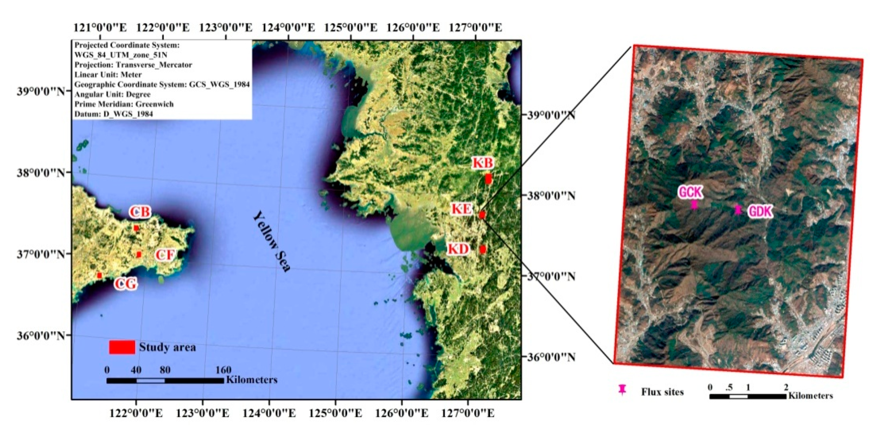
The time of sunrise, sunset was obtained from (http://www.sunrisesunset.com/). Daily maximum LST, maximum wind speed, mean wind speed, minimum air temperature, and maximum air temperature at 6 km resolution were obtained from the China Meteorological Administration (http://new-cdc.cma.gov.cn). Meteorological data were resized, using the nearest neighbor method, to either 50 or 250 m to match the spatial resolution of the GF-4 and MODIS imagery, respectively. The flux data of GDK and GCK sites were provided by Korea Flux Monitoring Network (KoFlux), they were used to verify simulated ET, with a 30 min measuring interval. The position of GDK is 37°44′56″ N, 127°08′57″ E, and the position of GCK is 37°44′54″ N, 127°09′44″ E (Figure 1). More details about GDK and GCK sites can be obtained from Asia Flux website (http://asiaflux.net/).

2.1.3. Location and Study Area

The study area is located in China and South Korea (Figure 1). The study area ranges from an altitude of 100 m–1100 m, comprising a hilly area and regions of flat terrain. Climatologically, it belongs to the north temperate continental monsoon climate, and experiences distinct seasonal variation as well as impacts from the monsoon advancing and retreating. To minimize the influences of undulating terrain and hill shade, six study areas were selected: (CB) mainly cultivated land and built-up areas, (CG) mainly of garden and urban construction land, (CF) mainly cultivated land and forest land, (KB) mainly cultivated land and village construction land, (KE) mainly forest land and river wetland (GDK and GCK Flux sites were in KE region), and (KD) mainly cultivated land and forest land (Figure 1).

2.2. Methods

2.2.1. SEBAL Model

The SEBAL model is a physically based land surface energy balance model that uses remotely sensed input and has been widely used to calculate ET [28,29,30,31,32]. Input data to the SEBAL model include: ground elevation, visible light and near infrared bands from remote sensing images (used to calculate the Normalized Difference Vegetation Index, NDVI value), the thermal infrared band (used to calculate the Land Surface Temperature, LST), and temperature and wind speed at the imaging time. The two papers were referred for the sensible heat calculation, hot and cold pixel selection, net radiation and soil head flux calculation [33,34]. Then, we calculated the ET of MODIS and GF-4 at imaging time in Table 2 using SEBAL model.

2.2.2. Calculation of NDVI

The MODIS NDVI was calculated by [35]:

$$NDVI=\frac{{\rho }_{nir}-{\rho }_{red}}{{\rho }_{nir}+{\rho }_{red}},$$

(1)

in Equation (1), the NDVI denotes the normalized vegetation index, and ${\rho }_{nir}$ and ${\rho }_{red}$ denote surface reflectance in the near infrared band and the red band, respectively.

The GF-4 NDVI was calculated as for the MODIS NDVI, shown in Equation (1), but the apparent reflectance of the near infrared (the red band) was derived by [36]:

$${\rho }_{\lambda }=\frac{\pi L_{\lambda }{d}^2}{\cos {\theta }_{s}ESU{N}_{\lambda }}$$

(2)

in Equation (2), where ${\rho }_{\lambda }$is the at-satellite reflectance, $ESU{N}_{\lambda }$ is the mean solar exoatmospheric irradiance in W·(m²·ster·μm)⁻¹, θ_s is the solar zenith angle in degrees, and d is the earth-sun distance in astronomical units. $L_{\mathsf{\lambda }}$is the at-satellite spectral radiance in W·(m²·ster·μm)⁻¹. θ_s can be obtained from the head file. The ESUN value for each GF-4 band has not been published yet, but can be calculated using the spectral response function of the solar spectrum curve and the sensor, as shown in Equation (3) [37].

$$ESUN=\frac{{\int }_{{\lambda }_1}^{{\lambda }_2}E\left(\lambda \right)S\left(\lambda \right)d_{\lambda }}{{\int }_{{\lambda }_1}^{{\lambda }_2}S\left(\lambda \right)d_{\lambda }},$$

(3)

In Equation (3), ESUN denotes the band average solar radiation outside of the atmosphere; λ₁ and λ₂ denote the upper and the lower integration limit of wavelength of band range; E(λ) denotes the solar spectrum radiation of the remote sensor out of the atmosphere at band λ, where different solar spectrum curves have different E(λ) values. Current studies show that the World Radiation Center (WRC) solar spectrum curve is the most favorable for the calculation of the ESUN using this sensor at a medium resolution in China [38]. According to the WRC solar spectrum curve, the E(λ) value could be in the range of λ₁ and λ₂; and S(λ) denotes the spectral response function of the remote sensor at band λ. The ESUN values for all GF-4 bands calculated using Equation (3) are shown in

Table 3. Calculated ESUN values for all GF-4 bands.

Bands	B1	B2	B3	B4	B5
ESUN W·(m2·ster·μm)−1	1609.81	1634.44	1839.33	1578.12	1104.77

.

The equation converting the DN value of satellite images to radiance images using the absolute calibration coefficient is [39]:

$$L_{\lambda }=A\times DN,$$

(4)

where GF-4 provides gain values (A) under 5 statuses, for example, status 2-6-4-6-6 denotes an integration time for full color, blue, green, red, and near infrared of 2, 6, 4, 6, and 6 ms, respectively, the other statuses please see

Table 4. Gain values of all GF-4 bands under different statuses.

Status	Gain Values (A)
	B1	B2	B3	B4	B5
2-6-4-6-6	0.5215	0.9400	0.9885	0.7847	0.5641
4-16-12-16-16	0.3100	0.3484	0.3484	0.3095	0.2257
6-20-16-20-20	0.1681	0.3263	0.2472	0.2806	0.1997
6-40-30-40-40	0.1681	0.1252	0.1226	0.1102	0.0796
6-30-20-30-30	0.1235	0.1784	0.1878	0.1515	0.1080

. Users need to determine the status of image bands according to the appropriate XML file parameters of GF-4 images, and then select the corresponding calibration coefficient.

2.2.3. Calculation of Land Surface Temperature

Unlike MODIS, GF-4 has no thermal infrared band to directly obtain LST at imaging time. Thus, in order to attain the LST of GF-4 at imaging time, it is necessary to utilize two daily LST images to simulate LST at any time using following equations [40,41,42]. In this paper, two daily LST images after sunrise were as input from MODIS (Table 1).

Daytime LST variation after sunrise was derived by:

$$T\left(t\right){=T}_{B,\mathit{set}}{+(T}_{B,\mathit{max}}{-T}_{B,\mathit{set}})\times \sin (W_2{t+\phi }_2),$$

(5)

in which: $T\left(t\right)$ denotes the LST at the time t; T_B,set denotes the LST at sunset; T_B,max denotes the daily maximum LST; W₂ = π/(DL − 2p) denotes the angular frequency of the sinusoid in the second stage; DL denotes the daytime length; p = TIME_x − NOON, TIME_x denotes the time when the maximum LST appears, TIME_x can be attained from meteorological stations, NOON denotes the time when the largest solar altitude appears, which is usually selected as 12.0; and φ₂ = π/2 − W₂ × TIME_x denotes the phase angle.

$$T_{B,\mathit{set}}=\frac{{4p\times T}_{B,\mathit{max}}+\left(\mathit{DL}-2p\right){\times T}_{B,\mathit{min}}}{\mathrm{DL}+2p},$$

(6)

This paper used the MODIS LST at the overpass time as inputs to calculate T_B,max, T_B,min, and T_B,set, and then calculated the LST at GF-4 imaging time using Equations (5) and (6).

2.2.4. Calculation of Daytime Air Temperature

Since GF-4 do not take images at night, the general formula to calculate daytime air temperature is [42]:

$$T_a=T_{min}+(T_{max}-T_{min})\times S(t),$$

(7)

in which T_a denotes daytime air temperature, and T_min and T_max denote daily minimum and daily maximum air temperature. In Equation (11), S(t) is a function of time (t) with data range of 0–1, represented as:

$$S\left(t\right)=\sin (\pi \times \frac{t-\mathrm{NOON}-\frac{\mathit{DL}}{2}}{\mathit{DL}+2P}),$$

(8)

in which t denotes any time, NOON denotes the time when the largest solar altitude appears, DL denotes the daytime length, and P denotes the time difference between the highest air temperature and the largest solar altitude. The time difference results from the intrinsic difference in heat storage of soil and air. When air temperature rises, T_min denotes the lowest air temperature at present day in Equation (11); when air temperature decreases, T_min denotes the lowest air temperature on the next day.

2.2.5. Calculation of Wind Speed

Daily variation in wind speed has the following features: the wind speed is low from nighttime to a time (t₁) in the morning, at which point the wind speed gradually increases to the maximum value until a time (t₂) in the afternoon, then gradually decreases to the minimum value until a time (t₃) at night. The t₁, t₂, and t₃ vary with location: in the study area, t₁ = 1.0, t₂ = 14.0, and t₃ = 0.0, and the variation of wind speed with time is expressed by the following equation [42]:

$$W_a=W_{min}+W_{max}\times \sin (2\mathsf{\pi }\times \frac{t_a{-tw}_{1,2}}{{\mathrm{SF}}_{1,2}}),$$

(9)

in which: W_a denotes wind speed at any time (m/s), W_max and W_min denote daily maximum and daily minimum wind speed (m/s), respectively, t_a denotes any time, tw₁ = t₁, tw₂ = 2(t₂ − t₃), SF₁ = 4(t₂ − t₁), and SF₂ = 4(t₃ − t₂).

The daily minimum wind speed can be calculated by using the daily air movement distance and the daily maximum wind speed as input data:

$$W_{min}=\frac{1000\times \left[TO{T}_w-W_{max}\times \left(S{F}_1+S{F}_2\right)\times 3600/2000/3.1415926\right]}{24.0\times 3600.0},$$

(10)

in Equation (10): TOT_w denotes daily air movement distance (km/d), which can be calculated from the daily average wind speed (m/s) available from meteorological stations and the length of a day (24 h × 3600 s/h).

2.2.6. Verification and Evaluation of Simulation Results

We estimated ET from SEBAL model using MODIS and GF-4 at imaging time in Table 2 per minute by using the methods in Section 2.2. The following methods were used for verifying ET: (1) cross-validation ET obtained from different remote sensing data; (2) verify with ET data measured in field. In this paper, we first cross-verified ET of GF-4at 11:36 (T₈) using ET of MODIS at 11:35 (MT₀). Then ET at 13:50 (${\mathrm{T}}_5^{\prime }$) of GF-4 and 13:45 (${\mathrm{MT}}_1^{\prime }$) of MODIS were cross-verified. Finally, we used the field measured ET data to verify them from the Flux sites in South Korea, which was close to the imaging time of remote sensing images. Since the measuring time interval at KoFlux sites was 30 min, we chose the measured ET at 11:30 and 14:00 to verify the simulated ET at 11:22 (${\mathrm{T}}_4^{\prime }$) and 13:58 (${\mathrm{T}}_7^{\prime }$) of GF-4 respectively. Then, the field measure ET at 12:00 (${\mathrm{MT}}_0^{\prime }$) was used to verify the simulated ET of MODIS at 12:10 (${\mathrm{MT}}_0^{\prime }$).

In order to evaluate the difference between measured ET and remote sensing data, we use root mean square error (RMSE) and mean relative error (MRE) to analyze the error.

$$\mathrm{RMSE}=\sqrt{\frac{{\sum }^{}{(Y_i-Y_i^{\prime })}^2}{N}},$$

(11)

$$\mathrm{MRE}=\sqrt{\frac{{\sum }^{}{[(Y_i-Y_i^{\prime })/Y_i^{\prime }]}^2}{N}},$$

(12)

in Equations (11) and (12), Y_i is the measured value, Y_i′ is the simulated value obtained from the model, and n is the number of sample points [43,44]. The smaller the values of RMSE and MRE, the higher the simulation accuracy of the model [43,44].

3. Results

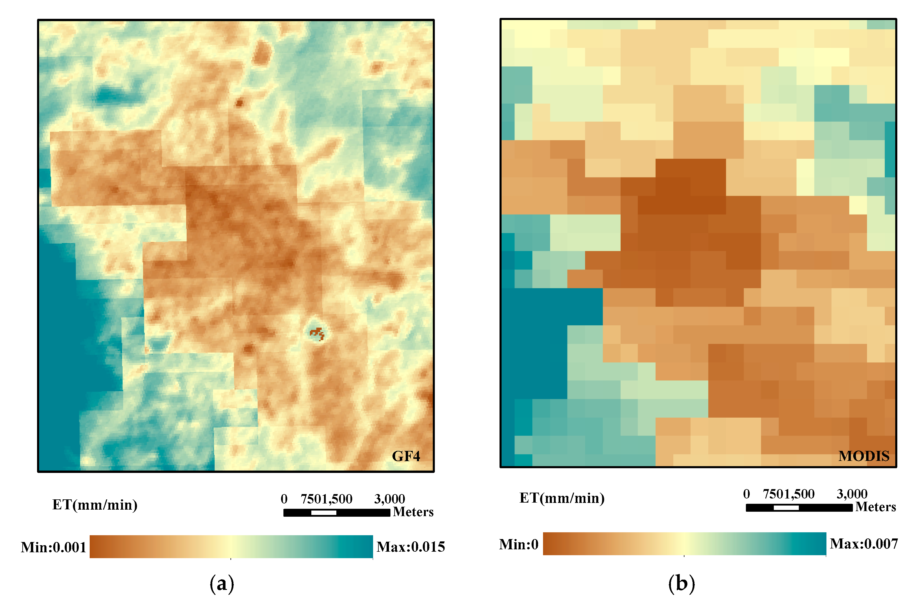
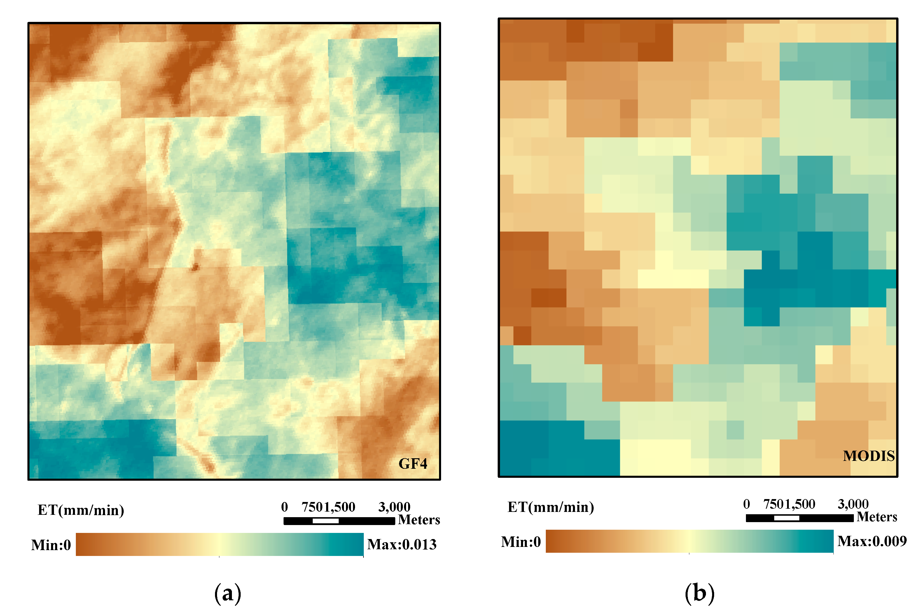
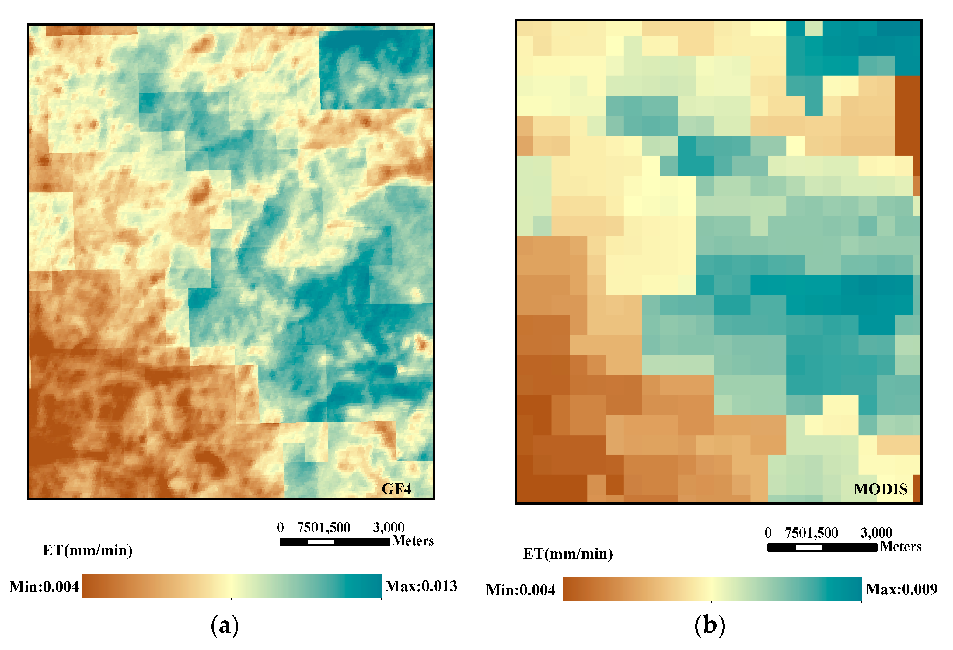
When the NDVI of GF-4 is taken as the input of SEBAL model, the spatial resolution of ET is 50 m, while when NDVI of MODIS is taken as the input of SEBAL model, the spatial resolution of ET is 250 m. Figure 2, Figure 3 and Figure 4 were the comparison of ET at 11:36 (T₈) of GF-4 and ET at 11:35 (MT₀) of MODIS in CB, CF and CG regions, respectively.

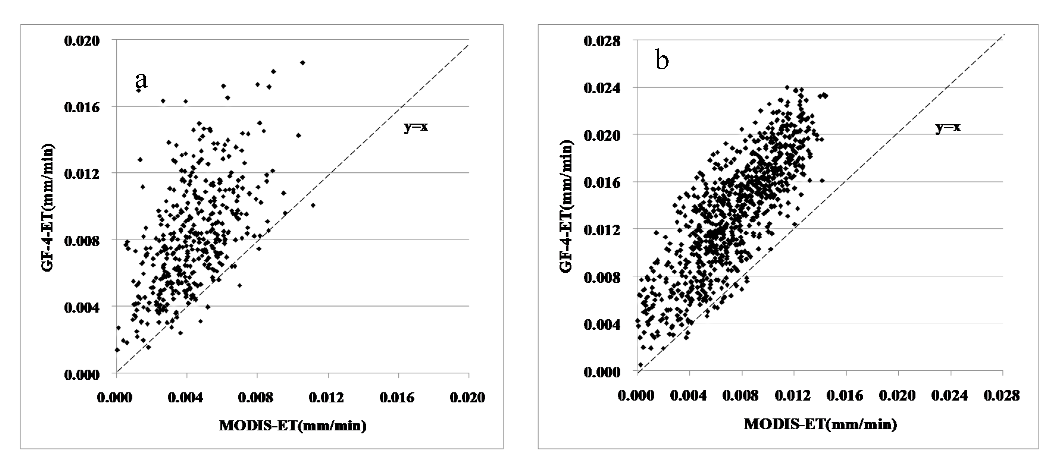
As seen in Figure 2, Figure 3 and Figure 4, since the spatial resolution of NDVI of GF-4 is higher than that of MODIS, the derived texture of ET is more obvious than that from MODIS. In order to cross-verify ET obtained from MODIS and GF-4, the bilinear method was used and the GF-4 ET data were resampled to 250 m, which was identical to the spatial resolution of MODIS. 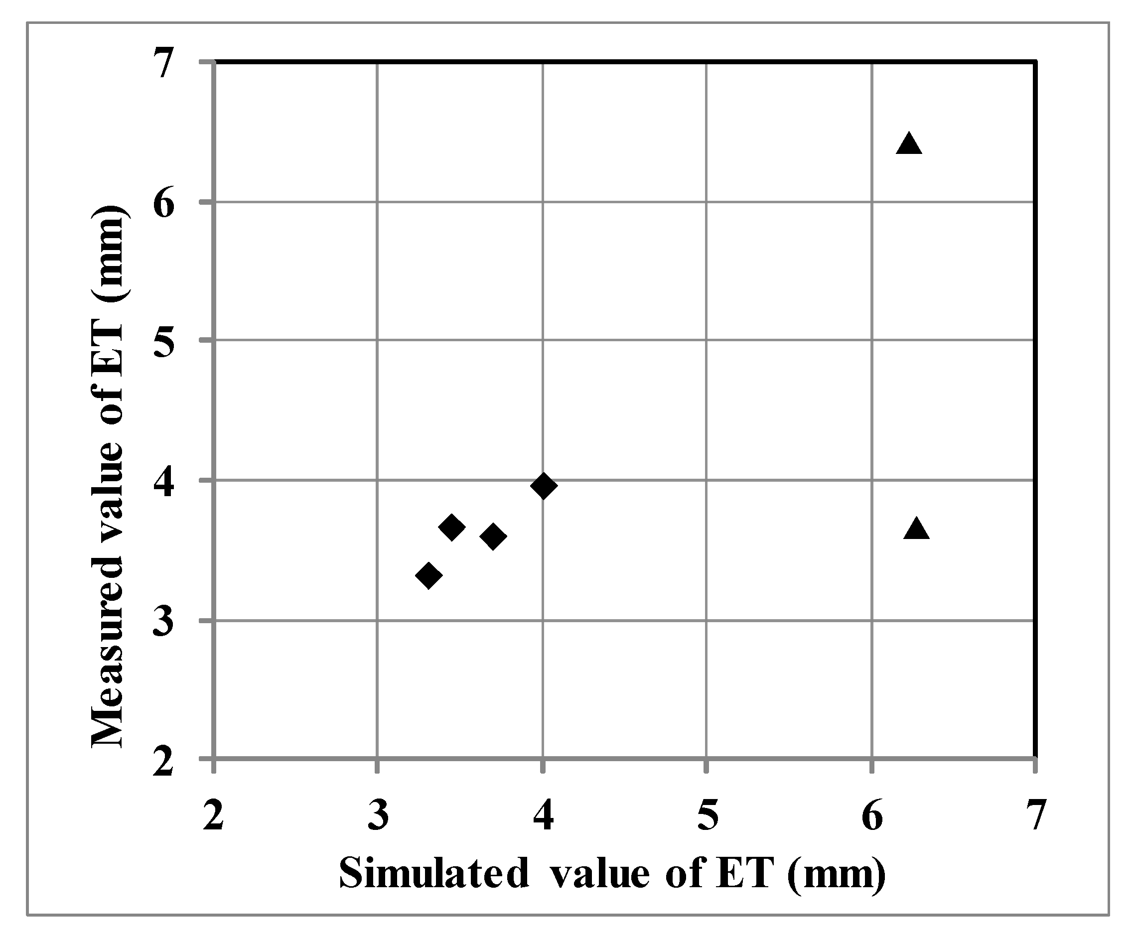As shown in Figure 5, 420 total sampling points were randomly selected in areas CB, CG and CF (Figure 5a), and 870 total sampling points were randomly selected in areas KB, KE and KD (Figure 5b) to find variability between the two ETs. Meanwhile we verified the simulated ET with the measured ET data of KoFlux as shown in Figure 6.

As can be seen from Figure 5, most ET simulation values of MODIS are less than that of GF-4’s, but there is a strong correlation between the ET derived from GF-4 and MODIS, R = 0.581 (p < 0.001) in areas CB, CG and CF, and R = 0.810 (p < 0.001) in areas KB, KE and KD. While the difference in imaging time of MODIS and that of GF-4 is 1 to 5 min, it is certain that the ETs derived from both satellites have a significant linear correlation at the same imaging time. In addition, as can be seen from Figure 6, the difference between the simulated and measured values of ET was not obvious.

The following two methods were used to verify the simulated ET. Firstly, we used the field measured data of KoFlux to verify the simulated ET of MODIS and GF-4. Then, we took the ET calculated by MODIS as the measured value, and the ET calculated by GF-4 as the simulated value. The verification results were shown in

Table 5. Using Flux data and MODIS to verify the accuracy of simulated ET.

Region	Data of Verification	MRE (%)	RMSE (mm/min)
KE	KoFlux data	16.95	0.00072
CB, CG and CF	MODIS	48.64	0.00451
KB, KE and KD	MODIS	48.33	0.00655

.

As can be seen from Figure 6 and Table 5, RMSE = 1.04 (mm/day) and the MRE was 16.95% when validating simulated ET values using KoFlux data, which showed that it was feasible to simulate ET using the methods in this paper, while most GF-4 simulated ET values were higher than those of MODIS’s, the MRE of ET when validating GF-4 using MODIS was less than 50%.

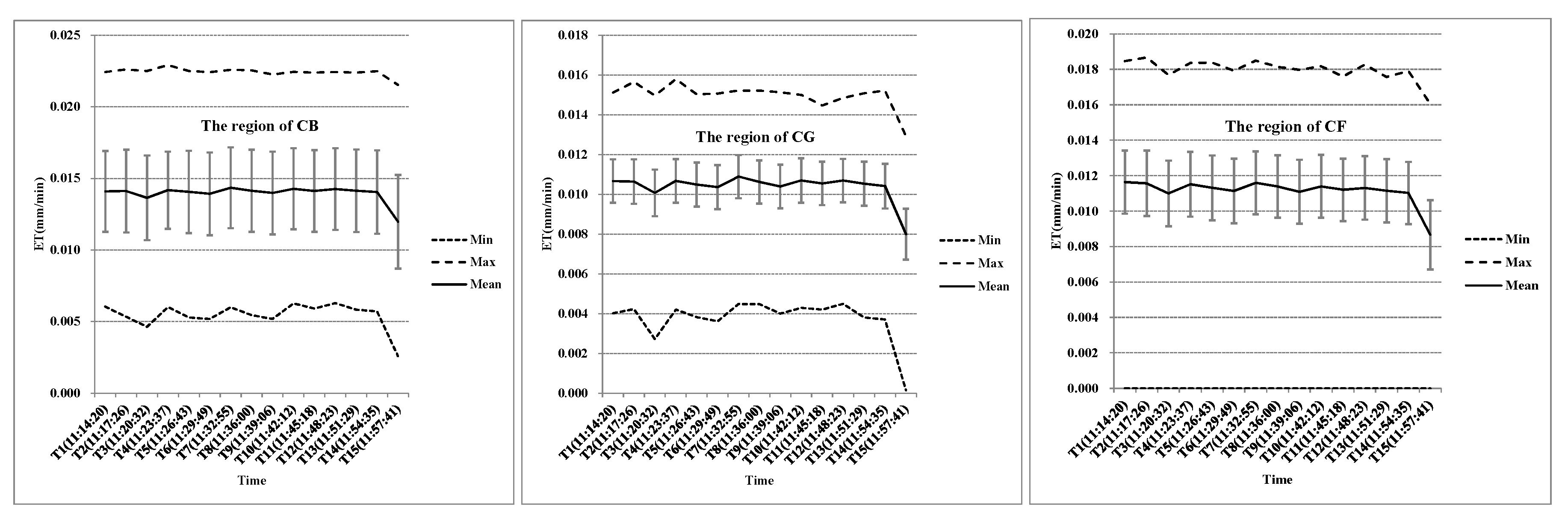
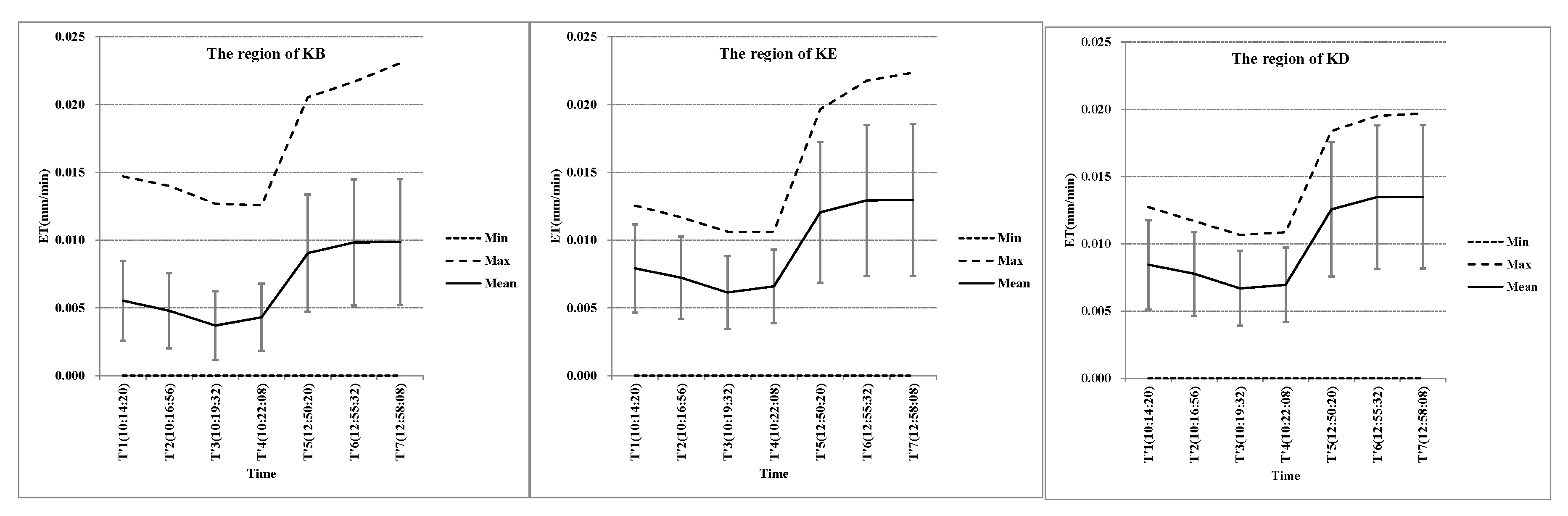
In order to further analyze the variation of ET in all study areas at time T₁–T₁₅ in areas CB, CG and CF, ${\mathrm{T}}_1^{\prime }-{\mathrm{T}}_7^{\prime }$in areas KB, KE and KD, the minimum, maximum, and average values, and the standard error of ET at above time was calculated by ArcMAP 10.3 for all pixels, as shown in Figure 7 and Figure 8.

As shown in Figure 7, the trends of the average, minimum, maximum and average ET in different study areas have significant differences, but the minimum ET in areas CF at time T₁–T₁₅ does not. The minimum ET does not vary in study area at time T₁–T₁₅, and the pixel with ET = 0 always exists. As shown in Figure 7 and Figure 8, the maximum value trend in all areas is the same as that of the average values, while the fluctuation in trend of the maximum and minimum value in all areas is different. This is mainly due to the difference among soil types and meteorological conditions in the six areas, causing the impacts on ET to vary [3,45]. This validates that due to the different of surface types and meteorological conditions, even two MODIS remote sensing images show daily variation in remote sensing pixel ETs. This daily variation does not follow the constant linear rule, meaning that extrapolating instantaneous ET at the imaging time to a hourly or daily time scale will cause relatively large errors [46,47]. Although GF-4 has no thermal infrared band and the LST at imaging time could not be obtained, its temporal resolution is relatively high and the land surface ET at a three-minute time interval can be attained by using all available meteorological and MODIS data. By using this method, the error associated with extrapolating instantaneous ET from one remote sensing image could be avoided and the real spatial diversity of ET at various imaging time could be obtained.

4. Discussion

While this paper compared ETs derived from GF-4 and MODIS using the SEBAL model, the extent of the differences from SEBAL model ET input data needs further analysis. The reason for the difference in ET simulation results between the two sensors needs further discussion, and the validation of ET simulation results requires careful consideration as well:

(1) Errors in SEBAL model input data lead to a decrease in ET simulation accuracy. However, in many areas, simulation is limited by available data, and often, the wind speed, LST, air temperature, and other data cannot be attained. While simulating the above parameters using the present model, various kinds of error must exist. If the above meteorological data could be replaced by observed data, the model accuracy could be significantly improved. In addition, the ESUN of GF-4 is not published yet, and the subsequent ESUN simulation that was used has errors which affected both the calculation of NDVI and the simulated values of ET.

(2) Besides the errors associated with SEBAL input data, the dependence on remote sensing data can lead to different ETs derived from the GF-4 and MODIS sensors. Many researchers have pointed out that the local variables of the SEBAL model would change with the scope of the remote sensing image, which could lead to additional uncertainty associated with the domain dependence of the remote sensing model accuracy [7,28,34,48]. On the other hand, remote sensing images with different spatial resolutions would also cause differences in local variables, and thus could lead to completely different dry-wet conditions, dependent upon the resolution of the remote sensing models. For all established models based on remote sensing images, the model outputs may have uncertainties if the determination of variables or input parameters depends on the scope and resolution of those images.

(3) The objective of this paper was not to validate whether the GF-4 or MODIS remote sensor has higher accuracy in ET retrieval, but to quantify the similarities and differences between ETs derived from both satellites by comparing their retrievals. It is clear that more efficient ground observations are essential to validate model results. Currently, widely used ET remote sensing model validation techniques include the lysimeter method, the field water balance method, the Bowen ratio method, the eddy covariance method and the large aperture scintillometer method [23,49,50,51,52]. However, in practical operation, the spatio-temporal scale of the observed data does not always match with that of the model retrievals. Therefore, we can only use KoFlux data with 2–10 minutes difference in remote sensing images for verification. The GF-4 is only the beginning of high orbit and high temporal-spatial resolution satellite technology, and as more research and data are gathered, new observational approaches will emerge.

(4)It is also necessary to consider cross-validation using remote sensing data with higher spatial resolution. We tried to verify GF-4 imaged at 11:14 in regions CB, CG and CF by using Landsat 8 imaged at 10:29. Meanwhile in regions KB, KE and KD, Landsat 8 imaged at 10:04 was used to verify GF-4 imaged at 11:14, the verification results of ET were shown in

Table 6. Using Landsat 8 data to cross-verify the simulated ET of GF-4.

Region	Data of Verification	MRE (%)	RMSE (mm/min)
CB, CG and CF	Landsat 8	79.21	0.00462
KB, KE and KD	Landsat8	190.36	0.00383

.

As can be seen from Table 6, when the simulated ET of GF-4 was verified by Landsat 8, the MRE of ET of GF-4 was very large. The imaging time of Landsat 8 was 44 min earlier than that of GF-4 in regions CB, CG and CF, and the imaging time of Landsat 8 was 70 min earlier than that of GF-4 in region KB, KE and KD. With such a long time difference, we think that the results of Table 6 can not accurately represent the actual accuracy of GF-4. However there is still a strong correlation between the ET derived from GF-4 and Landsat 8, R = 0.548 (p < 0.001).

5. Conclusions

(1) The spatial distribution of ET derived from MODIS and GF-4 showed that the texture of ET derived from GF-4 was more obvious than that from MODIS, and GF-4 was able to express the variability of ET spatial distribution. The correlation between ETs derived from two sensors showed significant linear correlation; and the ET values derived from GF-4 were higher than that of MODIS.

(2) Even in the same study area, trends in the maximum value, the average value, and the standard error of ET at different times were not the same. This validates that even if in two MODIS remote sensing images scope, due to different surface types and meteorological conditions, the daily variation of ET in the remote sensing pixel scale does not follow the constant linear rule.

(3) Since the temporal resolution of GF-4 is 3 minutes in our paper, the land surface ET every three-minutes could be obtained by using all available meteorological data and other remote sensing data. At this scale, the extrapolation of instantaneous ET from a single image was avoided, and the spatial diversity at each imaging time was attained.

(4) This paper has validated ET derived from GF-4 and MODIS, and the verification results also showed that the error was within the normal range, but more observational methods to validate ET estimation results of GF-4 are needed, which should be a major goal for future studies.

6. Perspectives

The GF-4 satellite can not only collect images with a large scope and at high temporal and spatial resolutions, but can also carry out “staring observation” in a specific region according to user instructions, which will play an important role in disaster reduction, meteorology, earthquake, forestry, and obtaining precise measurements in other fields. For example, GF-4 could practically observe a typhoon, since middle and low orbit satellites have high spatial resolution, but the retrogression time is relatively long, and the continuous observation of interesting areas is difficult. Compared with present high orbit continuous observation meteorological satellites, GF-4 could not only continuously provide information on the development of a typhoon, but could also take observations and measurements of details like typhoon textures.

In addition, GF-4 will further accelerate the development of advanced models supported by remote sensing data. Currently, models in disparate fields such as ecology, hydrology, geochemistry, and meteorology are driven by remote sensing data, but are limited by the temporal and spatial resolution of available remote sensing data, and face issues of fulfilling simultaneous goals such as having “short time”, “high accuracy”, and “large space” [53,54,55]. Most models driven by remote sensing are on time scales of days, months, or years. Even if a part of these models could realize hourly time scales from meteorological satellites such as those available from NOAA, the spatial resolution of their simulation results is over 1 km, which could not accurately estimate the spatial diversity of observation pixels [56,57,58]. The comprehensive advantages of GF-4 of increased temporal and spatial resolution and large widths would facilitate the appearance of various kinds of remote sensing models on fine time scales at minutes or even seconds.

References

- Wei, Z.; Yoshimura, K.; Wang, L.; Miralles, D.G.; Jasechko, S.; Lee, X. Revisiting the contribution of transpiration to global terrestrial evapotranspiration. Geophys. Res. Lett. 2017, 44, 2792–2801. [Google Scholar] [CrossRef]
- Borges Júnior, J.C.F.; Pinheiro, M.A.B. Daily Reference Evapotranspiration Based on Temperature for Brazilian Meteorological Stations. J. Irrig. Drain. Eng. 2019, 145, 04019029. [Google Scholar] [CrossRef]
- Karimi, S.; Kisi, O.; Kim, S.; Nazemi, A.H.; Shiri, J. Modelling daily reference evapotranspiration in humid locations of South Korea using local and cross-station data management scenarios. Int. J. Climatol. 2017, 37, 3238–3246. [Google Scholar] [CrossRef]
- Karlsen, R.H.; Bishop, K.; Grabs, T.; Ottosson-Löfvenius, M.; Laudon, H.; Seibert, J. The role of landscape properties, storage and evapotranspiration on variability in streamflow recessions in a boreal catchment. J. Hydrol. 2019, 570, 315–328. [Google Scholar] [CrossRef]
- Lian, X.; Piao, S.; Huntingford, C.; Li, Y.; Zeng, Z.; Wang, X.; Ciais, P.; McVicar, T.R.; Peng, S.; Ottle, C. Partitioning global land evapotranspiration using CMIP5 models constrained by observations. Nat. Clim. Chang. 2018, 8, 640–646. [Google Scholar] [CrossRef]
- Zhang, B.; He, C.; Di, X.; Li, F. Methods to estimate daily evapotranspiration from hourly evapotranspiration. Biosyst. Eng. 2017, 153, 129–139. [Google Scholar] [CrossRef]
- Bastiaanssen, W.G.M.; Noordman, E.J.M.; Pelgrum, H.; Davids, G.; Thoreson, B.P.; Allen, R.G. SEBAL model with remotely sensed data to improve water-resources management under actual field conditions. J. Irrig. Drain. Eng. 2005, 131, 85–93. [Google Scholar] [CrossRef]
- Awada, H.; Ciraolo, G.; Maltese, A.; Provenzano, G.; Hidalgo, M.A.M.; Còrcoles, J.I. Assessing the performance of a large-scale irrigation system by estimations of actual evapotranspiration obtained by Landsat satellite images resampled with cubic convolution. Int. J. Appl. Earth Obs. Geoinf. 2019, 75, 96–105. [Google Scholar] [CrossRef]
- Ramírez-Cuesta, J.M.; Cruz-Blanco, M.; Santos, C.; Lorite, I.J. Assessing reference evapotranspiration at regional scale based on remote sensing, weather forecast and GIS tools. Int. J. Appl. Earth Obs. Geoinf. 2017, 55, 32–42. [Google Scholar] [CrossRef]
- Talsma, C.; Good, S.; Miralles, D.; Fisher, J.; Martens, B.; Jimenez, C.; Purdy, A.J.R.S. Sensitivity of Evapotranspiration Components in Remote Sensing-Based Models. Remote Sens. 2018, 10, 1601. [Google Scholar] [CrossRef]
- He, M.; Kimball, J.S.; Yi, Y.; Running, S.W.; Guan, K.; Moreno, A.; Wu, X.; Maneta, M. Satellite data-driven modeling of field scale evapotranspiration in croplands using the MOD16 algorithm framework. Remote Sens. Environ. 2019, 230, 111201. [Google Scholar] [CrossRef]
- Zhao, J. Estimate Hourly and Daily Evapotranspiration Using Remote Sensing Technology for Haihe River Basin. Master’s Thesis, Twente Universiteit, Enschede, The Netherland, February 2017. [Google Scholar]
- Anderson, M.; Diak, G.; Gao, F.; Knipper, K.; Hain, C.; Eichelmann, E.; Hemes, K.S.; Baldocchi, D.; Kustas, W.; Yang, Y. Impact of Insolation Data Source on Remote Sensing Retrievals of Evapotranspiration over the California Delta. Remote Sens. 2019, 11, 216. [Google Scholar] [CrossRef]
- Knipper, K.R.; Kustas, W.P.; Anderson, M.C.; Alfieri, J.G.; Prueger, J.H.; Hain, C.R.; Gao, F.; Yang, Y.; McKee, L.G.; Nieto, H. Evapotranspiration estimates derived using thermal-based satellite remote sensing and data fusion for irrigation management in California vineyards. Irrig. Sci. 2019, 37, 431–449. [Google Scholar] [CrossRef]
- Mahmoud, S.H.; Gan, T.Y. Irrigation water management in arid regions of Middle East: Assessing spatio-temporal variation of actual evapotranspiration through remote sensing techniques and meteorological data. Agric. Water Manag. 2019, 212, 35–47. [Google Scholar] [CrossRef]
- Glenn, E.P.; Neale, C.M.U.; Hunsaker, D.J.; Nagler, P.L. Vegetation index-based crop coefficients to estimate evapotranspiration by remote sensing in agricultural and natural ecosystems. Hydrol. Process. 2011, 25, 4050–4062. [Google Scholar] [CrossRef]
- Foster, T.; Gonçalves, I.Z.; Campos, I.; Neale, C.M.U.; Brozović, N. Assessing landscape scale heterogeneity in irrigation water use with remote sensing and in situ monitoring. Environ. Res. Lett. 2019, 14. [Google Scholar] [CrossRef]
- Dalezios, N.R.; Blanta, A.; Loukas, A.; Spiliotopoulos, M.; Faraslis, I.N.; Dercas, N. Satellite methodologies for rationalising crop water requirements in vulnerable agroecosystems. Int. J. Sustain. Agric. Manag. Inform. 2019, 5, 37–58. [Google Scholar] [CrossRef]
- Ochoa-Sánchez, A.; Crespo, P.; Carrillo-Rojas, G.; Sucozhañay, A.; Célleri, R. Actual evapotranspiration in the high Andean grasslands: A comparison of measurement and estimation methods. Front. Earth Sci. 2019, 7, 55. [Google Scholar] [CrossRef]
- Carlson, T.N.; Petropoulos, G.P. A new method for estimating of evapotranspiration and surface soil moisture from optical and thermal infrared measurements: The simplified triangle. Int. J. Remote Sens. 2019, 40, 7716–7729. [Google Scholar] [CrossRef]
- Alfieri, J.G.; Kustas, W.P.; Anderson, M.C. A Brief Overview of Approaches for Measuring Evapotranspiration. Agroclimatol. Link. Agric. Clim. 2020, 60, 109–127. [Google Scholar] [CrossRef]
- Pützc, T.; Hannesd, M.; Wollschlägere, U. Estimating precipitation and actual evapotranspiration from precision lysimeter measurements. Procedia Environ. Sci. 2013, 19, 543–552. [Google Scholar] [CrossRef]
- Rosa, R.; Dicken, U.; Tanny, J. Estimating evapotranspiration from processing tomato using the surface renewal technique. Biosyst. Eng. 2013, 114, 406–413. [Google Scholar] [CrossRef]
- Liu, R.; Wen, J.; Wang, X.; Hu, Z.Y.; Kang, Y. Hourly variation of evapotranspiration estimated by visible infrared and microwave data over the northern Tibetan Plateau. J. Infrared Millim. Waves 2015, 34, 211–217. [Google Scholar] [CrossRef]
- Liu, Y.; Yao, L.; Xiong, W.; Zhou, Z. GF-4 Satellite and Automatic Identification System Data Fusion for Ship Tracking. IEEE Geosci. Remote Sens. Lett. 2019, 16, 281–285. [Google Scholar] [CrossRef]
- Liu, J.; Zheng, G.; Yang, J.; Wang, J. Top Cloud Motion Field of Typhoon Megi-2016 Revealed by GF-4 Images. IEEE Trans. Geosci. Remote Sens. 2019, 57, 4427–4444. [Google Scholar] [CrossRef]
- Wang, M.; Cheng, Y.; Tian, Y.; He, L.; Wang, Y. A New On-Orbit Geometric Self-Calibration Approach for the High-Resolution Geostationary Optical Satellite GaoFen4. IEEE J. Sel. Top. Appl. Earth Obs. Remote Sens. 2018, 11, 1670–1683. [Google Scholar] [CrossRef]
- Li, S.; Zhao, W. Satellite-based actual evapotranspiration estimation in the middle reach of the Heihe River Basin using the SEBAL method. Hydrol. Process. 2010, 24, 3337–3344. [Google Scholar] [CrossRef]
- Bastiaanssen, W.G.M.; Menenti, M.; Feddes, R.A.; Holtslag, A.A.M. A remote sensing surface energy balance algorithm for land (SEBAL). 1. Formulation. J. Hydrol. 1998, 212, 198–212. [Google Scholar] [CrossRef]
- Timmermans, W.J.; Kustas, W.P.; Anderson, M.C.; French, A.N. An intercomparison of the Surface Energy Balance Algorithm for Land (SEBAL) and the Two-Source Energy Balance (TSEB) modeling schemes. Remote Sens. Environ. 2007, 108, 369–384. [Google Scholar] [CrossRef]
- Grosso, C.; Manoli, G.; Martello, M.; Chemin, Y.; Pons, D.; Teatini, P.; Piccoli, I.; Morari, F. Mapping Maize Evapotranspiration at Field Scale Using SEBAL: A Comparison with the FAO Method and Soil-Plant Model Simulations. Remote Sens. 2018, 10, 1452. [Google Scholar] [CrossRef]
- Gobbo, S.; Lo Presti, S.; Martello, M.; Panunzi, L.; Berti, A.; Morari, F. Integrating SEBAL with in-Field Crop Water Status Measurement for Precision Irrigation Applications—A Case Study. Remote Sens. 2019, 11, 2069. [Google Scholar] [CrossRef]
- Rahimzadegan, M.; Janani, A. Estimating evapotranspiration of pistachio crop based on SEBAL algorithm using Landsat 8 satellite imagery. Agric. Water Manag. 2019, 217, 383–390. [Google Scholar] [CrossRef]
- Yang, Y.; Zhou, X.; Yang, Y.; Bi, S.; Yang, X.; Liu, D.L. Evaluating water-saving efficiency of plastic mulching in Northwest China using remote sensing and SEBAL. Agric. Water Manag. 2018, 209, 240–248. [Google Scholar] [CrossRef]
- Huete, A.; Didan, K.; Miura, T.; Rodriguez, E.P.; Gao, X.; Ferreira, L.G. Overview of the radiometric and biophysical performance of the MODIS vegetation indices. Remote Sens. Environ. 2002, 83, 195–213. [Google Scholar] [CrossRef]
- Li, G.; Li, X.; Li, G.; Wen, W.; Wang, H.; Chen, L.; Yu, J.; Deng, F. Comparison of Spectral Characteristics Between China HJ1-CCD and Landsat 5 TM Imagery. IEEE J. Sel. Top. Appl. Earth Obs. Remote Sens. 2013, 6, 139–148. [Google Scholar] [CrossRef]
- Pandya, M.R.; Singh, R.P.; Murali, K.R.; Babu, P.N.; Kirankumar, A.S.; Dadhwal, V.K. Bandpass solar exoatmospheric irradiance and Rayleigh optical thickness of sensors on board Indian remote sensing satellites-1B,-1C,-1D, and P4. IEEE Trans. Geosci. Remote Sens. 2002, 40, 714–718. [Google Scholar] [CrossRef]
- Zhang, L.; Shi, R.; Xu, Y.; Li, L.; Gao, W. Calculation of Mean Solar Exoatmospheric Irradiances of Several Sensors Onboard of Chinese Domestic Remote Sensing Satellites. J. Geo-Inf. Sci. 2014, 16, 621–627. (In Chinese) [Google Scholar] [CrossRef]
- Yang, A.; Zhong, B.; Wu, S.; Liu, Q. Radiometric cross-calibration of GF-4 in multispectral bands. Remote Sens. 2017, 9, 232. [Google Scholar] [CrossRef]
- Cong, Z.T. Study on the Coupling between the Winter Wheat Growth and the Water-Heat Transfer in Soil-Plant-Atmosphere Continuum. Ph.D. Thesis, Tsinghua University, Beijing, China, June 2003. [Google Scholar]
- Parton, W.J.; Logan, J.A. A model for diurnal variation in soil and air temperature. Agric. Meteorol. 1981, 23, 205–216. [Google Scholar] [CrossRef]
- Ephrath, J.E.; Goudriaan, J.; Marani, A. Modelling diurnal patterns of air temperature, radiation wind speed and relative humidity by equations from daily characteristics. Agric. Syst. 1996, 51, 377–393. [Google Scholar] [CrossRef]
- Trajkovic, S.; Gocic, M.; Pongracz, R.; Bartholy, J. Adjustment of Thornthwaite equation for estimating evapotranspiration in Vojvodina. Theor. Appl. Climatol. 2019, 138, 1231–1240. [Google Scholar] [CrossRef]
- Khedkar, D.; Singh, P.; Bhakar, S. Estimation of evapotranspiration using neural network approach. J. Agrometeorol. 2019, 21, 233–235. [Google Scholar]
- Wang, S.; Fu, B.J.; Gao, G.Y.; Yao, X.L.; Zhou, J. Soil moisture and evapotranspiration of different land cover types in the Loess Plateau, China. Hydrol. Earth Syst. Sci. 2012, 16, 2883–2892. [Google Scholar] [CrossRef]
- Ebenezer, A.O.; Okogbue Emmanuel, C.; Akinluyi Frank, O. Mapping evapotranspiration for different landcover in the Lake Chad region of Nigeria using landsat datasets. J. Remote Sens. Technol. 2016, 4, 58–69. [Google Scholar] [CrossRef]
- Peng, L.; Zeng, Z.; Wei, Z.; Chen, A.; Wood, E.F.; Sheffield, J. Determinants of the ratio of actual to potential evapotranspiration. Glob. Chang. Biol. 2019, 25, 1326–1343. [Google Scholar] [CrossRef]
- Long, D.; Singh, V.P. A modified surface energy balance algorithm for land (M-SEBAL) based on a trapezoidal framework. Water Resour. Res. 2012, 48, 2528. [Google Scholar] [CrossRef]
- Qiu, G.Y.; Momii, K.; Yano, T.; Lascano, R.J. Experimental verification of a mechanistic model to partition evapotranspiration into soil water and plant evaporation. Agric. For. Meteorol. 1999, 93, 79–93. [Google Scholar] [CrossRef]
- Pelosi, A.; Medina, H.; Villani, P.; D’Urso, G.; Chirico, G.B. Probabilistic forecasting of reference evapotranspiration with a limited area ensemble prediction system. Agric. Water Manag. 2016, 178, 106–118. [Google Scholar] [CrossRef]
- Lee, Y.; Kim, S. The modified SEBAL for mapping daily spatial evapotranspiration of South Korea using three flux towers and terra MODIS data. Remote Sens. 2016, 8, 983. [Google Scholar] [CrossRef]
- VH da Motta Paca, V.H.; Espinoza-Dávalos, G.E.; Hessels, T.M.; Moreira, D.M.; Comair, G.F.; Bastiaanssen, W.G. The spatial variability of actual evapotranspiration across the Amazon River Basin based on remote sensing products validated with flux towers. Ecol. Process. 2019, 8, 6. [Google Scholar] [CrossRef]
- Lees, K.J.; Quaife, T.; Artz, R.R.E.; Khomik, M.; Clark, J.M. Potential for using remote sensing to estimate carbon fluxes across northernpeatlands—A review. Sci. Total Environ. 2018, 615, 857–874. [Google Scholar] [CrossRef] [PubMed]
- Frohn, R.C.; Lopez, R.D. Remote Sensing for Landscape Ecology: New Metric Indicators for Monitoring, and Assessment of Ecosystems; CRC Press: Boca Raton, FL, USA, 2017. [Google Scholar]
- Lekula, M.; Lubczynski, M.W. Use of remote sensing and long-term in-situ time-series data in an integrated hydrological model of the Central Kalahari Basin, Southern Africa. Hydrogeol. J. 2019, 27, 1541–1562. [Google Scholar] [CrossRef]
- Fallahi, S.; Amanollahi, J.; Tzanis, C.G.; Ramli, M.F. Estimating solar radiation using NOAA/AVHRR and ground measurement data. Atmos. Res. 2018, 199, 93–102. [Google Scholar] [CrossRef]
- Chao, Y.; Farrara, J.D.; Zhang, H.; Armenta, K.J.; Centurioni, L.; Chavez, F.; Girton, J.B.; Rudnick, D.; Walter, R.K. Development, implementation, and validation of a California coastal ocean modeling, data assimilation, and forecasting system. Deep Sea Res. Part II Top. Stud. Oceanogr. 2018, 151, 49–63. [Google Scholar] [CrossRef]
- Ford, T.W.; Quiring, S.M. Comparison of Contemporary In Situ, Model, and Satellite Remote Sensing Soil Moisture With a Focus on Drought Monitoring. Water Resour. Res. 2019, 55, 1565–1582. [Google Scholar] [CrossRef]
© 2020 by the authors. Licensee MDPI, Basel, Switzerland. This article is an open access article distributed under the terms and conditions of the Creative Commons Attribution (CC BY) license (http://creativecommons.org/licenses/by/4.0/).