Abstract
Bicycles and motorcycles are characterized by large rider-to-vehicle mass ratios, thus making estimation of the rider’s inertia especially relevant. The total inertia can be derived from the body segment inertial properties (BSIP) which, in turn, can be obtained from the prediction/regression formulas available in the literature. Therefore, a parametric multibody three-dimensional rider model is devised, where the four most-used BSIP formulas (herein named Dempster, Reynolds-NASA, Zatsiorsky–DeLeva, and McConville–Young–Dumas, after their authors) are implemented. After an experimental comparison, the effects of the main posture parameters (i.e., torso inclination, knee distance, elbow distance, and rider height) are analyzed in three riding conditions (sport, touring, and scooter). It is found that the elbow distance has a minor effect on the location of the center of mass and moments of inertia, while the effect of the knee distance is on the same order magnitude as changing the BSIP data set. Torso inclination and rider height are the most relevant parameters. Tables with the coefficients necessary to populate the three-dimensional rider model with the four data sets considered are given. Typical inertial parameters of the whole rider are also given, as a reference for those not willing to implement the full multibody model.
Keywords:
rider; body segment inertial parameters; biomechanics; human body; motorcycle; bicycle; multibody 1. Introduction
It is well-known that motorcycles and bicycles are characterized by a large rider-to-vehicle mass ratio. On motorcycles, this ratio is usually in the range of 0.25–0.35, the lower figure being related to heavy bikes and the upper to sport bikes; while, on bicycles, the ratio is always greater than one. The inertial properties of the rider are, thus, especially relevant when it comes to dynamic simulations, such as those carried out in a multibody environment for handling and stability analyses of the vehicle–rider system [1,2,3,4,5,6].
Historically, motorcycle–rider and bicycle–rider systems have been simulated by considering the rider to be rigidly fixed to the chassis, while it has now become standard to consider the rider ‘suspended’ on the chassis (with springs tuned to give the typical frequencies and damping ratios of riders) with their hands interacting with the handlebar [7,8,9,10,11,12,13,14,15,16,17,18,19,20]. Regardless of the approach (i.e., fixed or suspended rider), estimation of the rider’s inertial properties is necessary in both cases. Moreover, in the most advanced motorcycle driving simulators [21,22,23,24,25,26,27], the contribution of the rider’s motion on the saddle to the vehicle dynamics are accounted for. Most of the time, such motion is monitored by cameras. The related inertial effects are introduced into the vehicle model after the inertial properties of the rider driving the simulator are assumed. Even in this case, estimation of the inertial properties is relevant.
There are different methods to estimate the body segment inertial parameters (BSIP) of a given subject [28,29,30,31,32,33,34], including direct measurements on cadavers [35,36,37] or photogrammetry and medical imaging on living humans [38,39,40,41,42,43,44,45,46,47,48]; however, they are more generally estimated by regression and scaling equations (which are derived from such measurements). The inertial properties of the whole body can, then, be computed after defining the subject’s posture. A practical approach is to build a three-dimensional multibody model of the whole human body, which consists of the body segments, properly connected to one another. The next step is defining the formulas to be used to estimate the properties of such segments.
A number of studies have been reported in the literature focused on the calculation of the inertial properties (e.g., mass, center of mass, moments of inertia, or gyration radii) and lengths of body segments of human bodies using regression/prediction formulas, which are given as functions of the mass and height (see, e.g., Reference [43,49,50,51,52,53,54,55,56]). Most of the time, the center of mass is assumed to lie on the longitudinal axis of each body segment, and the longitudinal and transverse axes are assumed principal of inertia.
The regression/prediction formulas of body segments in Reference [49] were derived based on the combination of the data sets in Reference [28,57]: the first considered a sample of American males in the age range of 20–40 years, while the second considered a random selection of adults, young males and females 20–30 years of age, some females in the 40–50 age bracket, and a number of subjects with disabilities in all age ranges. The center of mass was assumed along the longitudinal axis and a single gyration radius was given for each body segment.
Nine old male cadavers (average age 69) were used in Reference [50] to estimate the inertial properties of body segments from the human mass and height; a total of 14 body segments were considered (head, trunk, arms, forearms, hands, thighs, shanks, feet). This model is very popular for the two-dimensional estimation of inertial properties of human bodies. The center of mass was assumed along the longitudinal axis, but no moments of inertia were given (as they were deferred to future studies). This paper updates the results of Reference [35], which are still in use (see, e.g., Reference [33]), combined with those of Reference [58].
The lengths of body segments were obtained by combining the data of Reference [35,59,60,61] in Reference [51]. The location of the center of mass of each segment was derived from Reference [35,36,37,62,63], while the inertial properties were derived from Reference [37] (6 male cadavers, average age 54). The number of body segments is 14.
The data reported in Reference [36] were adjusted, in Reference [52], to reference the body segment proportions to joint centers, instead of the originally employed bony landmarks. The original data were taken by measuring thirteen cadavers; the body segments affected by these adjustments were the trunk, upper arms, forearms, thigh, and calves.
In Reference [53], the mean relative center of mass positions and radii of gyration reported by Reference [43] were adjusted, in order to reference them to the joint centers or other commonly used landmarks; 14 body segments were considered. The population consisted of 100 young males (average age 24) and 15 young females (average age 19), whose biomechanical properties were identified in-vivo by gamma-ray scanning techniques. Three gyration radii for each body segment were given and the center of mass was assumed to be aligned with the longitudinal axis of the segment.
In Reference [54,55], similarly to Reference [43,53], the data reported in Reference [39] (31 adult males, mean age 27.5) and [40] (46 women, mean age 31) were adjusted in order to reference them to the joint centers or other commonly used landmarks, according to the recommendations in Reference [64,65]. A relevant characteristic of these latter data sets is that they did not assume that the center of mass lay on the longitudinal axis of the segment, nor that the segment axes were principal of inertia. Therefore, the related regression/prediction formulas did not include such assumptions. Overall, 15 body segments were considered, as the trunk was divided in pelvis and torso. The body model was further updated in Reference [56], where an adjustment procedure to split the torso into thorax and abdomen segments was included.
When it comes to the literature specifically related to motorcycles, the works in Reference [18,19] are considered two classics. In Reference [19], data collected in vivo by the Japan Automobile Research Institute and data from cadavers of Reference [37] were combined to estimate the distribution of mass in 15 body segments. The resulting positions of the centers of mass and moments of inertia of riders were obtained by means of photographic measurements of rider positions. In Reference [18], an experimental characterization of 35 riders was carried out, with the locations of footrest, saddle, and handgrip corresponding to four motorcycles. The centers of mass and moments of inertia were given; however, the footpegs, saddle, and handgrip positions were not. Finally, in Reference [66], a multibody rider model was briefly described, although no reference to the data set used was given.
Regarding the literature specifically related to bicycles, in Reference [67], a rider model based on the mass data of Reference [35] and 31 grid points (mapping the skeleton of the rider and the bicycle) was presented. The inertial properties of each body segment, aligned along lines connected to appropriate grid points, was computed by assuming its shape (e.g., spheres and cuboids).
A review of the literature shows that at least three works have been alternatively widely employed for the estimation of the inertial properties of a human body in a generic configuration: Reference [50,51,53]. These are hereafter referred to as ‘Dempster-Model’, ‘Reynolds-NASA-Model’, and ‘Zatsiorsky–DeLeva-Model’, respectively, after their authors. In addition, the more recent [54,55] was also included in the multibody models considered, and is referred to as the ‘McConville–Young–Dumas’ model.
The aim of this work was to compare the four most widespread regression/prediction formulas available in the literature, in order to estimate the BSIP of human bodies in the case of the typical rider postures (sport, touring, and scooter). Unfortunately, such formulas are provided using different reference frames, landmarks, and even slightly different assumptions, thus making a direct comparison based only on their coefficients impossible. Therefore, a three-dimensional parametric multibody model is built, and the four selected regression/prediction formulas are adjusted to reference them to the same set of frames and landmarks. Tables are given to make it easier for other researchers to build the four models discussed in this work. As the target application is the estimation of the inertial properties of motorcycle and bicycle riders, the subject’s posture is defined by giving the location of the footpegs, saddle, and handgrips together with the torso inclination, the knee distance, and the elbow distance. However, the model can potentially also be used for car/truck drivers. In this latter scenario, the footpegs become the positions of feet near the gas and brake pedals, the saddle becomes the seat, the handgrips become the hand positions on the steering wheel, and the torso inclination becomes the inclination of the seat. The numerical findings of the numerical model are compared against experimental estimations of rider inertial properties, for validation purposes. Finally, a sensitivity analysis on the most important model parameters is carried out, in order to identify the most relevant factors and compare the trends provided by the four different models considered, as well as to compare the trends of the different data sets.
The work is organized as follows: In Section 2, the multibody model is built, while the model is validated against experiments in Section 3. Section 4 discusses the sensitivity analysis on the main model parameters, and Section 5 provides a set of baseline rider parameters for multibody simulations.
2. Multibody Model
The multibody model of the whole human body is built as an assembly of body segments, using the BSIP computed from the rider mass and height through four different regression/prediction formulas. In the following sections, the key aspects of the model are given, namely the frames and bodies used, the constraints and degrees of freedom considered, the data sets considered, and the implementation details.
2.1. Frames and Bodies
Whole-body inertial properties are usually given with respect to a reference frame centerd on the pelvis. Three planes are defined through such point for a standing body: the sagittal plane (body symmetry plane), the transverse plane (parallel to the floor), and the frontal or coronal plane (normal to the other two planes); see Figure 1a. The x-axis (sagittal axis) is the intersection between the sagittal and transverse plane and points forward, the z-axis (longitudinal axis) is the intersection between the sagittal and frontal plane and points upward, and the y-axis (transverse axis) is defined such that .
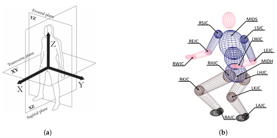
Figure 1.
Rider multibody model: reference frame for the whole body [51], with the sagittal (x), transverse (y), and longitudinal (z) axes and planes (a); and main points of the multibody model (b).
The multibody model of a human body consists of 14 body segments, namely trunk, forearms (), arms (), thighs (), shanks (), hands (), feet (), and head (including neck). Some authors have employed 16 segments by dividing the trunk into upper and lower trunk and not including the neck as part of the head. The location and orientation of each segment is defined using a reference frame centerd on the proximal point of the segment, as reported in Table 1. The reference frame of each body segment is parallel to that centerd in the pelvis, as shown in Figure 1a, when the human body is in the standard anatomical position (i.e., standing with the arms and legs parallel to the trunk and the palms pointing forward).

Table 1.
Proximal and distal points for each body segment. * indicates the origin of the reference frames attached to each body segment, while/indicates that the distal point is not defined, as it is not necessary for the model construction.
When the hands are placed on the handgrips, the x-axis (palm direction) points downward (vertically), the z-axis (fingers direction) points backward (horizontally), and the y-axis completes the frame. When the feet are on the footpegs, the x-axis points forward (horizontally), the z-axis upward (vertically), and the y-axis completes the frame.
2.2. Constraints
The multibody model consists of 84 unconstrained degrees of freedom (DOF), as there are 14 three-dimensional rigid bodies. The following points are introduced to define the configuration of the human body on the bike: the saddle point, the handgrip points (), and the footpeg points ().
The hands are fixed to the handlebar in the handgrip points, defined on the hands, and the feet are fixed to the chassis in the footpeg points, defined on the feet and, so, 24 DOF are constrained. The head center is fixed and aligned with the trunk’s longitudinal axis, at a given distance and, so, 6 DOF are constrained. All these fixed constraints are enforced by the following standard equations [68,69,70,71,72]:
where is the connection point on body i to which a frame with axes is attached, while is the connection point on body j to which a frame with axes is attached.
Spherical joints constrain the trunk to the arms on RSJC/LSJC and the forearms to the hands on RWJC/LWJC, constraining 12 DOF; see Figure 1b. Similarly, spherical joints constrain the thighs to the trunk on RHJC/LHJC and the shank to the feet on RAJC/LAJC, also constraining 12 DOF; see Figure 1b. The trunk is attached to the saddle point through a spherical joint, constraining 3 DOF. The equations related to all these 9 spherical joints are given as (1)–(3).
The arms are connected to the forearms through revolute joints centerd in REJC/LEJC, with the rotation axis perpendicular to the plane defined by SJC, EJC, and WJC, constraining 10 DOF. Similarly, the thighs are connected to the shanks through revolute joints centerd in RKJC/LKJC with the rotation axis perpendicular to the plane defined by HJC, KJC, and AJC, constraining 10 DOF. The equations related to these four revolute joints are given as (1)–(3), (5), and (6).
The remaining 7 DOF are the inputs for the numerical analyses (together with human height and mass) and can be related to the rotation of the trunk along the horizontal (roll), vertical (yaw), and transverse (pitch) axes through the saddle point; the distance between elbows and the distance between knees; and the distance between the right elbow and the sagittal plane and the distance between the right knee and the sagittal plane. In more detail, the trunk axes are constrained to have a fixed orientation with respect to the saddle point (and related frame), as follows:
where the indices i and j refer to the trunk and saddle frames, respectively, while , , and are the rider’s longitudinal lean (or pitch) angle, yaw angle, and roll angle, respectively, with respect to the saddle. The distance between elbows and knees and their position with respect to the sagittal plane are defined by the following equations:
where and are the left and right elbow points, is the distance between elbows, and is the distance between the right elbow and the sagittal plane, while and are the left and right knee points, is the distance between knees, and is the distance between the right knee and the sagittal plane. At this stage, the model is kinematically determinate.
2.3. Data Sets
The four most popular data sets reported in the literature were employed to compute the length of body segments, the location of the center of mass, and the moments of inertia. Details with the specific tables employed are reported in Appendix A, in order to make it easier to practically implement the model independently. Indeed, such data are spread throughout multiple references, which partially explains the confusion sometimes related to the definition of the exact sources employed for the computation of the inertial properties.
2.4. Implementation
The configuration of the multibody model is obtained by solution of the 84 non-linear algebraic equations associated to the constraints described in Section 2.2. The problem can either be solved using a root-finding solver or by implementation on one of the several available commercial multibody software packages. The authors decided to implement the model in the well-known Adams through a macro. Most constraints are standard and, thus, already available (e.g., fixed, spherical, and revolute joints); however, the related equations are given in Section 2.2, while others were written by hand using the function GCON (generic constraints). Again, such constraints are given in Section 2.2. The configuration was obtained without much trouble, with a solution error of in a number of steps which did not exceeds 50.
3. Validation
In this section, the numerical results of the multibody model described in Section 2 are compared against the experimental findings. The center of mass of nine riders (age in the range 24–27, mean body mass index (BMI) 23.87 kg/m with standard deviation 2.82 kg/m, mean height 1.76 m with standard deviation 0.05 m, mean mass 73.93 kg with standard deviation 6.87 kg, mean elbow distance 0.53 m with standard deviation 0.05 m, and knee distance 0.48 m, equal to the fuel tank width, for all riders) was measured in riding position using the testing rig developed at the University of Padova shown in Figure 2.
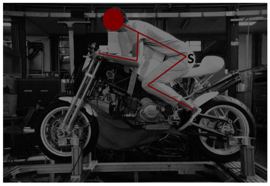
Figure 2.
A rider on the test rig, with the main kinematic points used in the multibody model indicated.
3.1. Test Procedure
The machine consisted of a rigid frame, four load cells (two fixed to the frame and two adjustable to fit the vehicle wheelbase), an inclinometer, and an hydraulic lifting system. The motorcycle was fixed to the load cells (two for each wheel) at the wheel axles. Both front and rear suspensions were locked, in order to avoid dynamic effects during measurements.
For the estimation of the center of mass components (horizontal and vertical , with respect to the rear wheel axle), the vehicle was pitched at different angles by lifting the rigid frame. For each position, a static measurement of the loads normal to the rigid frame (e.g., vertical when the pitch was zero) was taken and the results were interpolated as follows:
where w is the distance between the wheel axles, and are the front and rear loads (measured with the load cells), and is the vehicle pitch angle (measured with an inclinometer). The center of mass of the rider was obtained by subtraction of the measurement of the bike from the measurement of the bike and rider. Foam cushions between the trunk and the tank (visible in Figure 2) were employed to prevent involuntary rider motions when pitching the bike during the test, as well as to guarantee a comfortable riding position while standing in a static posture for a long time (the test duration was about 15 min). A sporty posture (mean lean angle 62 degrees with standard deviation 4.5 degrees) was chosen, allowing the rider to get a more sturdy leaning point on the bike, thus reducing vibration and, ultimately, yielding better measurements. For the same reasons, the maximum pitch angle during tests was limited to 16 degrees. The procedure consisted of 17 measures for each rider, from 0 degrees to 16 degrees and return, with steps of 2 degrees.
The elbow distance was measured during the test, in order to make sure that the rider kept a fixed posture with respect to the bike. Trunk lean angle and trochanter center position with respect to the saddle point were derived from photographic data. The photos taken (one at the beginning of each test) were elaborated to correct distortions and aberration phenomena. This was done by means of a reference photo depicting a chessboard, through which a scaling matrix (pixel to mm) was built using a standard open source software for image processing. As a further check, for each rider’s photo, three measures are verified: front and rear wheel radii and wheels axle distance. Finally, it was assumed that the rider’s sagittal plane was on the bike’s vertical symmetry plane. The model MIDH is the mean point between the right and left throcanter anatomical landmarks; see point S in Figure 2. Therefore, different riders had slightly different postures, although sitting on the same bike.
3.2. Data Analysis
The comparison between the numerical model results and the experimental data for the four data sets considered is reported in Figure 3. The test subjects were selected among the students of the Department of Industrial Engineering of University of Padova, who had experience in cycling and possibly in motorcycle riding. Estimation of the measurement errors was done by repeating the entire procedure with the same rider eight times and evaluating the standard deviations of the measured center of mass coordinates. The measurement error calculated for both the x and z components was equal to mm with a degree of confidence of 99.7%. These errors were assumed to be independent of the rider measured.
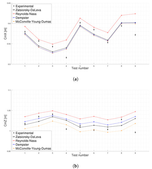
Figure 3.
Horizontal (a) and vertical (b) position of G: numerical vs. experimental.
The RMS of the difference (numerical vs. experimental) in the estimation of the center of mass x co-ordinate for the four data sets were: 4.72% for Reynolds-NASA, 2.78% for Dempster, 2.74% for Zatsiorsky–DeLeva, and 2.72% for McConville–Young–Dumas (with respect to the nominal experimental values). The RMS of the difference (numerical vs. experimental) in the estimation of the center of mass z co-ordinate for the four data sets were: 2.64% for Reynolds-NASA, 1.75% for Dempster, 1.66% for McConville–Young–Dumas, and 1.56% for Zatsiorsky–DeLeva (with respect to the nominal experimental values).
The simulated x co-ordinate of G was almost identical in all data sets, with the exception of Reynolds-NASA, which gave larger estimates (i.e., G shifted towards the front wheel). More than half of the experiments lay in between Reynolds-NASA and the other models, while the remaining experimental estimates were smaller (i.e., shifted towards the rear wheel) than all of the numerical estimates. The predictions of the four models were clearly distinguished from one another in the z co-ordinate. The tallest estimation was with Reynolds-NASA and the shortest with McConville–Young–Dumas, while the other two models lay in between. Two-thirds of the experiments lay in between the Reynolds-NASA and McConville–Young–Dumas models, while the remaining experiments were shorter than all the numerical estimates. The maximum difference between the simulations and experiments was 0.05 m (both horizontally and vertically), obtained with the Reynolds-NASA model (test 9).
4. Sensitivity Analysis
The multibody model was employed to investigate the effect of the main model parameters—namely knee distance, elbow distance, lean angle, and rider height—on the rider’s inertial properties. The rider’s yaw and roll ( and in (8) and (9)) were assumed to be zero, while the elbows and knees were assumed to be symmetric with respect to the sagittal plane ( and ). The analysis was performed over three different types of motorcycle: sport (tucked position), touring, and a scooter (upright position). A 74 kg rider was assumed, whose posture was defined with the parameters in Table 2. Four data sets were considered.
Table 2.
Baseline parameters for the rider on the three bikes. The coordinates are given with respect to the saddle point.
Sensitivity with respect to the rider mass was not considered, ase the center of mass does not change with it, while the gyration radii are linearly proportional to it. Indeed, the position of the whole center of mass can be computed from the positions of the center of mass of its i components :
The mass of each body segment is proportional to the whole-body mass m through the coefficient (Table A1, Table A2, Table A3 and Table A5), while the position of the center of mass of each body segment is proportional to the body segment length through the coefficients , , and (Table A1, Table A2, Table A3 and Table A5), when expressed in the local reference frame. The projection onto the global reference frame is obtained through a roto-translation matrix , which has the rotation matrix of the local reference frame in its upper-left corner (whose columns consist of the unit vectors of the local reference frame, expressed in the global reference frame) and the location of the origin of the reference frame in its fourth column (again expressed in the global frame); the (4,4) value is always one [1,70]. Finally, the length of the body segment is proportional to the body height h through the coefficient (Table A1, Table A2, Table A3 and Table A5). Equation (15) indicates that the position of the center of mass of the whole body only depends on the height (and, of course, on the data set selected for the coefficients , and ). Similarly, the whole-body inertia matrix, , can be obtained from the parallel axis theorem as:
where , and are the gyration radii in the segment reference frame, which are proportional to the segment length through the coefficients , and (Table A1 and Table A2, Table A4, Table A5, Table A6); is the identity matrix; and is the distance between the center of mass of the body segment and the whole center of mass
which has been shown to be dependent on h only; see (15). Therefore, given the data set of regression/prediction coefficients, the moments of inertia of the whole body are proportional to m (given the posture and height) and change with h (indeed, the posture changes with height).
4.1. Effect of Knees Distance
The knee distance was varied throughout the range 0.20–0.70 m in 0.01 m increments, keeping all other parameters constant. Figure 4 shows the variation of for the four data sets for each rider posture. When the knee distance increased, moved rearward in all bikes, while the vertical displacement depended on the bike. The mean variations (end-to-end) in the x direction were: −0.96 cm for sport posture, −1.08 cm for touring posture, and −1.31 cm for scooter posture. The mean variations in the z direction were: 0.70 cm for sport posture, 0.53 cm for touring posture, and −0.33 cm for scooter posture. Overall, the variation in the location of , as related to the variation of the knee distance, was of the same order of magnitude of the variation in the location of related to changes between McConville–Young–Dumas and Reynolds-NASA data sets (up to 4 cm).
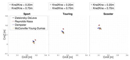
Figure 4.
Position of the center of mass as a function of knee distance.
Figure 5 shows the variation of the gyration radii for the four data sets for each rider posture. An increase of the knee distance corresponded to an increase of (roll) and (yaw)—as intuition suggests—while had a slightly decreasing trend. The mean variations (end-to-end) in were: 2.16 cm for sport posture, 1.46 cm for touring posture, and 2.36 cm for scooter posture. The mean variations in were: −0.32 cm for sport posture, −0.73 cm for touring posture, and −0.40 cm for scooter posture. The mean variations in were: 3.30 cm for sport posture, 3.44 cm for touring posture, and 2.06 cm for scooter posture. The variations of the components between models (up to 6 cm) were, again, on the same order of magnitude of the variations related to the knee distance. The model at the upper end depended on the component and posture selected, while the lower-end model was always the Dempster; probably due to the lack of local inertia tensors for body segments. As expected, on the sport bike, (roll) and (pitch) were minimum, due to the tucked position. The touring position had the maximum , due to the erect position (similarly to scooter), combined with the larger distance between saddle and footpegs.
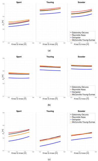
Figure 5.
Roll (a), pitch (b), and yaw (c) gyration radii as a function of knee distance.
4.2. Effect of Elbow Distance
The elbow distance was varied, in 0.01 m steps, throughout the range 0.30–0.70 m, keeping all other parameters constant. Figure 6 shows the variation of for the four data sets for each rider posture. With an increase in elbow distance, moved slightly upward, while the horizontal displacement depended on the posture (moved slightly rearward in touring and slightly forward in sport/scooter). The mean variations (end-to-end) in the x direction were: 0.08 cm for sport posture, −0.21 cm for touring posture, and 0.04 cm for scooter posture. The mean variations in the z direction were: 0.18 cm for sport posture, 0.15 cm for touring posture, and 0.25 cm for scooter posture. The variations in the location of related to the elbow distance were an order of magnitude smaller than the variations related to changes in the data set.
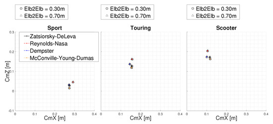
Figure 6.
Position of the center of mass as a function of elbow distance.
Figure 7 shows the variation of the gyration radii for the four data sets for each rider posture. An increase of the elbow distance value corresponded to a slight increase of and , while was almost independent from this parameter. The mean variations in were: 0.82 cm for sport posture, 0.69 cm for touring posture, and 0.75 cm for scooter posture. The mean variations in were: 0.06 cm for sport posture, 0.06 cm for touring posture, and 0.12 cm for scooter posture. The mean variations in were: 0.96 cm for sport posture, 1.08 cm for touring posture, and 0.96 cm for scooter posture.
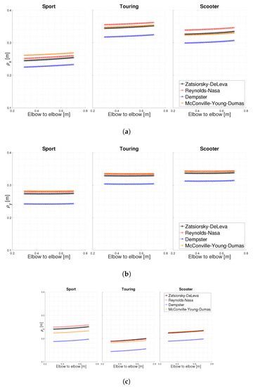
Figure 7.
Roll (a), pitch (b), and yaw (c) gyration radii as a function of elbow distance.
4.3. Effect of (Longitudinal) Lean Angle
The lean angle was varied, in 1 degree steps, throughout the range 45–85 degrees for sport posture, 5–45 degrees for touring posture, and from −5 (slightly leaned rearward) to +35 degrees for scooter posture, keeping all other parameters constant. Figure 8 shows the variation of for the four data sets for each rider posture. With an increase of the lean angle, moved significantly forward (except for the sport posture, due to the high lean angle values) and significantly downward (except for the scooter posture, due to the low lean angle values). The mean variations (end-to-end) in the x direction were: 6.09 cm for sport posture, 12.75 cm for touring posture, and 13.58 cm for scooter posture. The mean variations in the z direction were: −14.19 cm for sport posture, −6.79 cm for touring posture, and −4.10 cm for scooter posture. The variations of between models (up to 4 cm) were almost a third of the variations related to the lean angle.
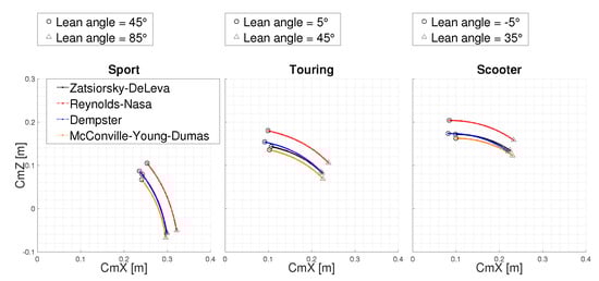
Figure 8.
Position of the center of mass as a function of lean angle.
Figure 9 shows the variation of the gyration radii for the four data sets for each rider posture. An increase in the lean angle value corresponded to a decrease of (roll) and (pitch)—as intuition suggests—while exhibited a decreasing behavior for small lean-angle values (<20 degrees) and then increased for high lean-angle values (>40 degrees). The mean variations (end-to-end) in were: −8.52 cm for sport posture, −4.95 cm for touring posture, and −2.98 cm for scooter posture. The mean variations in were: −4.74 cm for sport posture, −4.44 cm for touring posture, and −5.05 cm for scooter posture. The mean variations in were: 3.55 cm for sport posture, 1.18 cm for touring posture, and −3.07 cm for scooter posture.
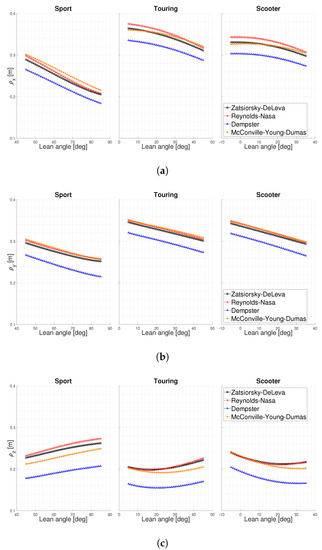
Figure 9.
Roll (a), pitch (b), and yaw (c) gyration radii as a function of lean angle.
4.4. Effect of Rider Height
The rider height was varied throughout the range 1.55–1.95 m in 0.01 m steps, keeping all other parameters constant. Figure 10 shows the variation of for the four data sets for each rider posture. When increasing the rider height, moved forward and upward, with a slope that depended on the rider posture (maximum for scooter and minimum with sport). The mean variations (end-to-end) in the x direction were: 5.88 cm for sport posture, 3.66 cm for touring posture, and 1.88 cm for scooter posture. The mean variations in the z direction were: 2.34 cm for sport posture, 4.67 cm for touring posture, and 6.40 cm for scooter posture. The variations of between models (up to 4 cm) were comparable with the variations related to the rider height.
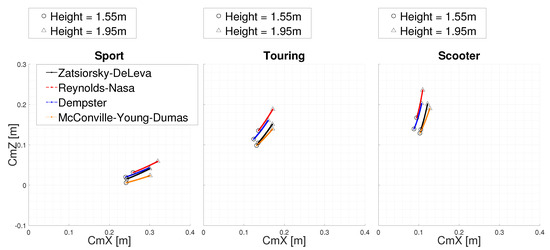
Figure 10.
Position of the center of mass as a function of rider height.
Figure 11 shows the variation of the gyration radii for the four data sets for each rider posture. An increase of rider height value corresponded to an increase of all components. The mean variations (end-to-end) in were: 2.27 cm for sport posture, 3.88 cm for touring posture, and 2.83 cm for scooter posture. The mean variations in were: 2.85 cm for sport posture, 4.06 cm for touring posture, and 3.59 cm for scooter posture. The mean variations in were: 2.29 cm for sport posture, 1.69 cm for touring posture, and 2.79 cm for scooter posture.
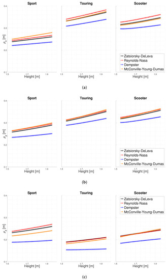
Figure 11.
Roll (a), pitch (b), and yaw (c) gyration radii as a function of rider height.
5. Baseline Parameters
Typical inertial parameters for sport, touring, and scooter postures are given in Table 3 for all four data sets considered, as a reference for multibody simulations. The posture parameters, the mass and height used, as well as the location of the saddle points, footpeg points, and handgrip points, are given in Table 2. For the four data sets considered, had the highest position in the case of the scooter and the lowest in the case of the sport posture; when it came to the horizontal position, the sequence of locations was scooter–touring–sport, when moving from the rear- to the front-end. The sport posture gave the minimum values of both roll and pitch gyration radii for all data sets, while the maximum values are obtained with the touring (maximum roll) and scooter (maximum pitch) postures, respectively. The touring posture also gave the minimum values for the pitch gyration radii.
Table 3.
Typical rider parameters for sport, touring, and scooter postures. coordinates are given with respect to the saddle reference frame.
In Reference [3], the typical sport rider gyration radii are given. The roll and pitch radii were in the range 0.23–0.28 m, which the values computed in this work fell within; see the sport column of Table 3. The yaw radius in Reference [3] was in the range 0.15–0.19 m, a bit smaller than the values computed in this work (all larger than 0.19 m); see again the sport column of Table 3.
The centers of mass, together with the roll and yaw moments of inertia, of 35 riders were measured in Reference [18], both in upright and leaned posture. The locations of footpegs, handgrips, and saddles were not given. For the upright posture, the mean coordinates were m and m (with respect to the saddle), while the mean gyration radii were m and m. These values were close to those reported in the scooter column of Table 3. For the leaned posture, the mean coordinates were m and m, while the computed mean gyration radii were m and m. These values were between those reported in the sport and touring columns of Table 3.
The rider posture of a typical bicycle rider was analyzed in Reference [67]. Comparison of the locations of the saddle, footpegs, and handgrips suggests that the posture was close to that of the touring vehicle considered in this work. Indeed, in Reference [67], the computed radii were m, m, and m, which were close to the values reported in the touring column of Table 3.
6. Discussion
The investigation carried out showed that there are four main BSIP formulas available and that such formulas need to be adjusted to a common set of frames and assumptions before being employed. After such an adjustment (see Appendix A), the BSIP coefficients are not far from one another and provide similar trends (although with slightly different figures) when varying the main posture parameters of motorcycle and bicycle riders. The numerical estimates provided in this work for baseline riders were consistent with those in similar studies reported in the literature. The minor effect related to elbow distance and the small effect related to knee distance suggest that the inertial estimation of riders based only on the height and lean is sufficient, in most cases. When it comes to the BSIP models selected, the ‘McConville–Young–Dumas’ model offers clearer implementation, together with the ‘Dempster’ model. The ‘Reynolds-NASA’ model requires the inspection of different sources, where there are different conventions even within the main source. The ‘Zatsiorsky–DeLeva’ model has some missing points and requires some assumptions during implementation. Finally, the ‘McConville–Young–Dumas’ model was the only model featuring a center of mass away from the longitudinal axis of the body segment and cross moments of inertia. However, such effects are secondary when compared with the transportation moments related to the parallel axis theorem.
7. Conclusions
The main BSIP prediction/regression formulas available in the literature were reviewed, with special emphasis on implementations for two-wheelers. A parametric rider model suitable for multibody applications has been developed. The BSIP prediction/regression formulas of the four most-used models were employed to investigate the estimation of the location of the center of mass and gyration radii. The location of the center of mass was also compared against experimental data on a sample of riders. It was found that all four BSIP data sets considered gave similar trends, although with slightly different figures. The sport posture had the minimum roll and pitch moments of inertia, the touring posture had the maximum roll, and the scooter posture had the maximum pitch moment of inertia. The elbow distance had a minor effect in the estimation of the location of the center of mass and the gyration radii, while the effect of the knee distance was on the same order of magnitude as changing the data set. The (longitudinal) lean angle and the rider height were the most relevant factors. Leaning forward lowers and moves forward the center of mass—this lowering is the main effect in the case of the sport motorcycle, while forward motion is the main effect in the case of touring and scooter postures. The lean angle also lowered the roll and pitch gyration radii, while the yaw gyration radius increased only for high values of lean angle (above 40 degrees). Increasing the height of the rider moved the center of mass forward and upward—the forward motion is the main effect in the case of the sport bike, while rising is the main effect in the case of the touring and scooter. Height also increased all gyration radii. Finally, typical parameters for a sport posture, touring posture, and scooter posture were provided.
This work, in addition to suggesting the main parameters to be considered when estimating the variation of the inertial properties of bicycle and motorcycle riders, provides tables for the implementation of the most popular BSIP formulas in a consistent set of frames and landmarks, in order to serve as a practical reference for future analyses by other researchers.
Author Contributions
Conceptualization, M.M. and N.P.; methodology, M.B., M.M. and N.P.; software, M.B.; validation, M.B. and M.M.; formal analysis, M.B. and M.M.; investigation, M.B. and M.M.; resources, M.M.; data curation, M.B.; writing—original draft preparation, M.B. and M.M.; writing—review and editing, M.B. and M.M.; visualization, M.B. and M.M.; supervision, M.M.; project administration, M.M. All authors have read and agreed to the published version of the manuscript.
Funding
This research received no external funding.
Conflicts of Interest
The authors declare no conflict of interest.
Appendix A
The coefficients of the data sets are reported in Table A1, Table A2, Table A3, Table A4, Table A5 and Table A6. Given a human body with height h and mass m, the length of segment i is , which has mass , center of mass in co-ordinate (expressed in the local reference frame), gyration radii of the main moments of inertia (again in the local reference), and the radii of the cross moments of inertia are (Dumas model only). Details on the specific models are given in the sections below.
Appendix A.1. Zatsiorsky–DeLeva Model Implementation
Most of the data necessary to build the Zatsiorsky-De Leva model are taken from Table 4 in Reference [53]. For arms, forearms, hands, thighs, shanks, and feet, the upper part of the table is used (male columns) without any adjustment, while alternative endpoints are selected for the head and trunk: the head is measured from the vertex to cervicale (CERV) and the trunk from CERV to MIDH. Implementation in the multibody model requires replacing CERV with MIDS: these two points are vertically aligned (along the trunk longitudinal axis) and their distance can be computed using Table 4 in Reference [53], which gives the trunk in terms of MIDS and MIDH.The HEEL point is not defined with respect to the shank endpoint (LMAL). However, this point is given in Reference [73], to which [53] also refers. In addition, the HEEL point is assumed to be vertically aligned with LMAL and shifted downward by half of the LMAL height, which is measured in Table 75 (male mean value has been used) of Reference [73]. The ratio, with respect to the foot length, is evaluated using Table 51, again from Reference [73]. Tables from Reference [73] are also used to estimate the lateral displacements of SJC and HJC with respect to MIDS and MIDH, respectively. The lateral displacement of SJC is assumed to be equal to half of the biacromial breadth (Table 10), while the lateral displacement of HJC is assumed to be equal to half of the bispinous breadth (Table 14). The ratios are evaluated using Table 99 for the stature. Handgrip points are assumed coincident with the hand endpoints, while footpeg points are assumed vertically aligned with LMAL and shifted downward of LMAL height (Table 75).
Table A1.
Zatsiorsky–DeLeva model parameters for each body segment.
Table A1.
Zatsiorsky–DeLeva model parameters for each body segment.
| Head and neck | 6.94 | 18.99 | 0 | 0 | 63.26 | 22.26 | 23.14 | 19.17 |
| Trunk | 43.46 | 29.61 | 0 | 0 | 56.90 | 38.39 | 35.81 | 19.78 |
| Arm | 2.71 | 16.18 | 0 | 0 | −57.72 | 28.50 | 26.90 | 15.80 |
| Forearm | 1.62 | 15.45 | 0 | 0 | −45.74 | 27.60 | 26.50 | 12.10 |
| Hand | 0.61 | 4.95 | 0 | 0 | −79.00 | 62.80 | 51.30 | 40.10 |
| Thigh | 14.16 | 24.25 | 0 | 0 | −40.95 | 32.90 | 32.90 | 14.90 |
| Shank | 4.33 | 24.93 | 0 | 0 | −44.59 | 25.50 | 24.90 | 10.30 |
| Foot | 1.37 | 14.82 | 44.15 | 0 | −12.44 | 12.40 | 24.50 | 25.70 |
Appendix A.2. Dempster Model Implementation
The data necessary to build the Dempster model are taken from Reference [50]. Mass percentages of body segments are taken from Table 4 (Dempster column), with the exception of the trunk coefficient, which is obtained by subtracting the other segments from the whole body; otherwise, the total mass is more than 100% (a well-known issue). The segments lengths and co-ordinate coefficients are taken from Tables 2 and 3 and Figure 3 in [50]. The trunk center of mass distance from MIDH is evaluated as the weighted average of thorax, shoulder, and lumbocoxal segment CoM positions. The gyration radii are not reported and, thus, are assumed to be zero. Handgrip points are assumed to be coincident with the hand centers of mass, while footpeg points are assumed coincident with AJC points.
Table A2.
Dempster model parameters for each body segment.
Table A2.
Dempster model parameters for each body segment.
| Head and neck | 7.92 | 20.33 | 0 | 0 | 63.85 | 0 | 0 | 0 |
| Trunk | 50.412 | 27.98 | 0 | 0 | 55.63 | 0 | 0 | 0 |
| Arm | 2.64 | 17.35 | 0 | 0 | −43.74 | 0 | 0 | 0 |
| Forearm | 1.531 | 15.72 | 0 | 0 | −42.93 | 0 | 0 | 0 |
| Hand | 0.612 | 3.422 | 0 | 0 | −100 | 0 | 0 | 0 |
| Thigh | 10.008 | 23.99 | 0 | 0 | −42.78 | 0 | 0 | 0 |
| Shank | 4.612 | 25.05 | 0 | 0 | −42.64 | 0 | 0 | 0 |
| Foot | 1.431 | 3.694 | 100 | 0 | 0 | 0 | 0 | 0 |
Appendix A.3. Reynolds-NASA Model Implementation
The data necessary to build the Reynolds-NASA model are taken from Reference [51,74]. Mass percentages of body segments are taken from Table 15 in Reference [51], while position and components are taken from Tables 12 and 28, respectively. For some body segments, the lengths given in these tables have different definitions (e.g., bone lengths instead of link lengths). Therefore, data are taken from Tables 1 and 3 in Reference [51] for the location of the center of mass and from tables in Reference [74] for the moments of inertia (the mean of the data contained in each table are used, taking into account only western males). As in the Zatsiorsky–DeLeva model, the heel is not defined with respect to the shank endpoint: similar assumptions are thus made. The heel point is assumed to be vertically aligned with AJC and shifted downward by half of the LMAL height, which is measured in Reference [74], Table 543. The ratio, with respect to the foot length, is evaluated using Table 362. The same reference is used to estimate the lateral displacements of SJC and HJC with respect to MIDS and MIDH, respectively. The lateral displacement of SJC is assumed to be equal to half of the biacromial breadth (Table 103), while the lateral displacement of HJC is assumed to be equal to half of the biliocristale breadth (Table 130). Handgrip points are assumed coincident with the hand centers of mass, while footpeg points are assumed to be vertically aligned with AJC and shifted downward of the LMAL height.
Table A3.
Reynolds-NASA model parameters for each body segment (mass, length, and center of mass).
Table A3.
Reynolds-NASA model parameters for each body segment (mass, length, and center of mass).
| Head and neck | 8.40 | 18.07 | 0 | 0 | 65.41 |
| Trunk | 50.00 | 29.31 | 0 | 0 | 58.00 |
| Arm | 2.80 | 0 | 0 | −48.00 | |
| Forearm | 1.698 | 0 | 0 | −41.00 | |
| Hand | 0.602 | 6.19 | 0 | 0 | −51.00 |
| Thigh | 10.00 | 0 | 0 | −41.00 | |
| Shank | 4.30 | 0 | 0 | −44.00 | |
| Foot | 1.40 | 15.18 | 44.00 | 0 | −12.80 |
Table A4.
Reynolds-NASA model parameters for each body segment (length and gyration radii).
Table A4.
Reynolds-NASA model parameters for each body segment (length and gyration radii).
| Head and neck | 11.14 | 31.60 | 30.90 | 34.20 |
| Trunk | 29.31 | 43.00 | 35.20 | 20.80 |
| Arm | 18.64 | 26.10 | 25.40 | 10.40 |
| Forearm | 15.17 | 29.60 | 29.20 | 10.80 |
| Hand | 5.00 | 50.40 | 45.60 | 26.60 |
| Thigh | 27.03 | 27.90 | 28.40 | 12.20 |
| Shank | 25.12 | 28.20 | 28.20 | 7.60 |
| Foot | 15.18 | 12.20 | 24.90 | 26.10 |
Appendix A.4. McConville–Young–Dumas Model Implementation
The data necessary to build the McConville–Young–Dumas model are taken from Tables 1 and 2 in Reference [54], along with the corrections in Reference [55]. Torso and pelvis body segments are combined into a single trunk element. All the frames in Reference [54] have the y-axis pointing upward and the x-axis pointing forward in the standard anatomical position: a 90 -degree rotation along the x-axis is applied to make it consistent with the convention of the multibody model. The trunk and head bodies are defined with respect to a frame located in the cervical joint center (CJC), while the MIDS point is required. MIDS is assumed to lie along the trunk longitudinal axis and translated downward, with respect to CJC, as reported in Table 2 of Reference [54]. Handgrip points are assumed coincident with the projection of the hand centers of mass along the hand longitudinal axes, while footpeg points are assumed to be vertically aligned with AJC and horizontally aligned with the foot centers of mass.
Table A5.
McConville–Young–Dumas model parameters for each body segment.
Table A5.
McConville–Young–Dumas model parameters for each body segment.
| Head and neck | 6.70 | 19.77 | 1.58 | −0.08 | 63.28 | 22.16 | 23.74 | 16.62 |
| Trunk | 47.50 | 28.14 | −2.26 | 0.17 | 56.24 | 36.79 | 37.14 | 22.91 |
| Arm | 2.40 | 15.31 | 1.70 | 2.60 | −45.20 | 33.00 | 32.00 | 14.00 |
| Forearm | 1.70 | 15.99 | 1.00 | −1.40 | −41.70 | 28.00 | 27.00 | 11.00 |
| Hand | 0.60 | 4.52 | 8.20 | −7.40 | −83.90 | 61.00 | 56.00 | 38.00 |
| Thigh | 12.30 | 24.41 | −4.10 | −3.30 | −42.90 | 29.00 | 30.00 | 15.00 |
| Shank | 4.80 | 24.46 | −4.80 | −0.70 | −41.00 | 28.00 | 28.00 | 10.00 |
| Foot | 1.20 | 10.34 | 38.20 | −2.60 | −15.10 | 17.00 | 36.00 | 37.00 |
Table A6.
McConville–Young–Dumas model parameters for each body segment (cross gyration radii).
Table A6.
McConville–Young–Dumas model parameters for each body segment (cross gyration radii).
| Head and neck | 1.58 | −2.37 | −5.54 |
| Trunk | −0.99 | 3.16 | 15.89 |
| Arm | −5.00 | −2.00 | 6.00 |
| Forearm | −2.00 | 8.00 | 3.00 |
| Hand | −15.00 | 20.00 | 22.00 |
| Thigh | 2.00 | 7.00 | 7.00 |
| Shank | 2.00 | −5.00 | −4.00 |
| Foot | 8.00 | 0 | 13.00 |
References
- Limebeer, D.J.N.; Massaro, M. Dynamics and Optimal Control of Road Vehicles; Oxford University Press: Oxford, UK, 2018. [Google Scholar]
- Kooijman, J.D.G.; Schwab, A.L. A review on bicycle and motorcycle rider control with a perspective on handling qualities. Veh. Syst. Dyn. 2013, 51, 1722–1764. [Google Scholar] [CrossRef]
- Cossalter, V. Motorcycle Dynamics, 2nd ed.; Lulu.com: Morrisville, NC, USA, 2006. [Google Scholar]
- Sharp, R.S.; Evangelou, S.; Limebeer, D.J.N. Advances in the modelling of motorcycle dynamics. Multibody Syst. Dyn. 2004, 12, 251–283. [Google Scholar] [CrossRef]
- Pacejka, H.; Besselink, I.J.M. Tire and Vehicle Dynamics, 3rd ed.; Butterworth-Heinemann: Oxford, UK, 2012. [Google Scholar]
- Cossalter, V.; Lot, R.; Massaro, M. An advanced multibody code for handling and stability analysis of motorcycles. Meccanica 2011, 46, 943–958. [Google Scholar] [CrossRef]
- Doria, A.; Marconi, E.; Massaro, M. Identification of rider’s arms dynamic response and effects on bicycle stability. In Proceedings of the AMSE IDETC International Design Engineering Technical Conferences & Computers and Information in Engineering Conference, St. Louis, MO, USA, 16–19 August 2020. [Google Scholar]
- Tomiati, N.; Colombo, A.; Magnani, G. A nonlinear model of bicycle shimmy. Veh. Syst. Dyn. 2019, 57, 315–335. [Google Scholar] [CrossRef]
- Uchiyama, H.; Tanaka, K.; Nakagawa, Y.; Kinbara, E.; Kageyama, I. Study on Weave Behavior Simulation of Motorcycles Considering Vibration Characteristics of Whole Body of Rider; SAE Technical Paper; SAE International: Warrendale, PA, USA, 2018. [Google Scholar]
- Klinger, F.; Nusime, J.; Edelmann, J.; Plöchl, M. Wobble of a racing bicycle with a rider hands on and hands off the handlebar. Veh. Syst. Dyn. 2014, 52, 51–68. [Google Scholar] [CrossRef]
- Massaro, M.; Cole, D.J. Neuromuscular-Steering Dynamics: Motorcycle Riders vs. Car Drivers. In Proceedings of the ASME 2012 5th Annual Dynamic Systems and Control Conference, Fort Lauderdale, FL, USA, 17–19 October 2012; pp. 217–224. [Google Scholar]
- Massaro, M.; Lot, R.; Cossalter, V.; Brendelson, J.; Sadauckas, J. Numerical and experimental investigation of passive rider effects on motorcycle weave. Veh. Syst. Dyn. 2012, 50, 215–227. [Google Scholar] [CrossRef]
- Doria, A.; Formentini, M.; Tognazzo, M. Experimental and numerical analysis of rider motion in weave conditions. Veh. Syst. Dyn. 2012, 50, 1247–1260. [Google Scholar] [CrossRef]
- Schwab, A.L.; Meijaard, J.P.; Kooijman, J.D.G. Lateral dynamics of a bicycle with a passive rider model: Stability and controllability. Veh. Syst. Dyn. 2012, 50, 1209–1224. [Google Scholar] [CrossRef]
- Plöchl, M.; Edelmann, J.; Angrosch, B.; Ott, C. On the wobble mode of a bicycle. Veh. Syst. Dyn. 2012, 50, 415–429. [Google Scholar] [CrossRef]
- Cossalter, V.; Doria, A.; Lot, R.; Massaro, M. The effect of rider’s passive steering impedance on motorcycle stability: Identification and analysis. Meccanica 2011, 46, 279–292. [Google Scholar] [CrossRef]
- Sharp, R.S.; Limebeer, D.J.N. On steering wobble oscillations of motorcycles. Proc. Inst. Mech. Eng. Part J. Mech. Eng. Sci. 2004, 218, 1449–1456. [Google Scholar] [CrossRef]
- Katayama, T.; Aoki, A.; Nishimi, T.; Okayama, T. Measurements of Structural Properties of Riders; SAE Technical Paper; SAE International: Warrendale, PA, USA, 1987. [Google Scholar]
- Nishimi, T.; Aoki, A.; Katayama, T. Analysis of Straight Running Stability of Motorcycles; SAE Technical Paper; SAE International: Warrendale, PA, USA, 1985; p. 856124. [Google Scholar]
- Cossalter, V.; Lot, R.; Massaro, M. The influence of frame compliance and rider mobility on the scooter stability. Veh. Syst. Dyn. 2007, 45, 313–326. [Google Scholar] [CrossRef]
- Cheng, J.; Su, H.; Chen, K. Driver Posture Detection Method in Motorcycle Simulator. In Proceedings of the 2019 International Conference on Artificial Intelligence and Advanced Manufacturing (AIAM), Dublin, Ireland, 17–19 October 2019; pp. 622–626. [Google Scholar]
- Nagasaka, K.; Ichikawa, K.; Yamasaki, A.; Ishii, H. Development of a Riding Simulator for Motorcycles; SAE Technical Papers; SAE International: Warrendale, PA, USA, 2018. [Google Scholar] [CrossRef]
- Will, S.; Schmidt, E.A. Powered two wheelers’ workload assessment with various methods using a motorcycle simulator. IET Intell. Transp. Syst. 2015, 9, 702–709. [Google Scholar] [CrossRef]
- Massaro, M.; Cossalter, V.; Lot, R.; Rota, S.; Ferrari, M.; Sartori, R.; Formentini, M. A portable driving simulator for single-track vehicles. In Proceedings of the 2013 IEEE International Conference on Mechatronics (ICM), Vicenza, Italy, 27 February–1 March 2013; pp. 364–369. [Google Scholar] [CrossRef]
- Stedmon, A.W.; Brickell, E.; Hancox, M.; Noble, J.; Rice, D. MotorcycleSim: A user-centerd approach in developing a simulator for motorcycle ergonomics and rider human factors research. Adv. Transp. Stud. 2012, 31–48. [Google Scholar] [CrossRef]
- Cossalter, V.; Lot, R.; Massaro, M.; Sartori, R. Development and validation of an advanced motorcycle riding simulator. Proc. Inst. Mech. Eng. Part J. Automob. Eng. 2011, 225, 705–720. [Google Scholar] [CrossRef]
- Nehaoua, L.; Arioui, H.; Mammar, S. Review on single track vehicle and motorcycle simulators. In Proceedings of the 2011 19th Mediterranean Conference on Control Automation (MED), Corfu Island, Greece, 20–23 June 2011; pp. 940–945. [Google Scholar]
- Drillis, R.; Contini, R. Body Segment Parameters; Technical Report 116.03; New York Univ. School of Engineering and Science: New York, NY, USA, 1964. [Google Scholar]
- Reid, J.G.; Jensen, R.K. Human body segment inertia parameters: A survey and status report. Exerc. Sport Sci. Rev. 1990, 18, 225–241. [Google Scholar] [CrossRef] [PubMed]
- Jensen, R.K. Human Morphology: Its role in the mechanics of movement. J. Biomech. 1993, 26, 81–94. [Google Scholar] [CrossRef]
- Pearsall, D.J.; Reid, G. The Study of Human Body Segment Parameters in Biomechanics: An Historical Review and Current Status Report. Sport. Med. Eval. Res. Exerc. Sci. Sport. Med. 1994, 18, 126–140. [Google Scholar] [CrossRef] [PubMed]
- Erdmann, W.S. Geometry and inertia of the human body-review of research. Acta Bioeng. Biomech. 1999, 1, 23–35. [Google Scholar]
- Winter, D.A. Biomechanics and Motor Control of Human Movement, 4th ed.; John Wiley & Sons: Hoboken, NJ, USA, 2009. [Google Scholar]
- Dumas, R.; Wojtusch, J. Handbook of Human Motion; chapter Estimation of the Body Segment Inertial Parameters for the Rigid Body Biomechanical Models Used in Motion Analysis; Springer International Publishing: Cham, Switzerland, 2017; pp. 1–31. [Google Scholar] [CrossRef]
- Dempster, W.T. Space Requirements of the Seated Operator; Technical Report WADC-TR-55-159; Wright Air Development Center, Wright-Patterson Air Force Base: Dayton, OH, USA, 1955. [Google Scholar]
- Clauser, C.E.; McConville, J.T.; Young, J.W. Weight, Volume and Center of Mass of Segments of the Human Body; Technical Report 69-70; Aerospace Medical Research Laboratories, Wright-Patterson Air Force Base: Dayton, OH, USA, 1969. [Google Scholar]
- Chandler, R.F.; Clauser, C.E.; McConville, J.T.; Reynolds, H.M.; Young, J.W. Investigation of Inertial Properties of the Human Body; Technical Report ADA016485; Air Force Aerospace Medical Research Lab Wright-Patterson AFB OH, Wright-Patterson Air Force Base: Dayton, OH, USA, 1975. [Google Scholar]
- Jensen, R.K. Estimation of the biomechanical properties of three body types using a photogrammetric method. J. Biomech. 1978, 11, 349–358. [Google Scholar] [CrossRef]
- McConville, J.T.; Churchill, T.D.; Kaleps, I.; Clauser, C.E.; Cuzzi, J. Anthropometric Relationships of Body and Body Segment Moments of Inertia; Technical Report AFAMRL-TR-80-119; Aerospace Medical Research Laboratory, Wright–Patterson Air Force Base: Dayton, OH, USA, 1980. [Google Scholar]
- Young, J.W.; Chandler, R.F.; Snow, C.C.; Robinette, K.M.; Zehner, G.F.; Lofberg, M.S. Anthropometric and Mass Distribution Characteristics of the Adults Female; Technical Report FA-AM-83-16; FAA Civil Aeromedical Institute: Oklaoma City, OK, USA, 1983.
- Ackland, T.R.; Blanksby, B.A.; Bloomfield, J. Inertial characteristics of adolescent male body segments. J. Biomech. 1988, 21, 319–327. [Google Scholar] [CrossRef]
- Mungiole, M.; Martin, P.E. Estimating segment inertial properties: Comparison of magnetic resonance imaging with existing methods. J. Biomech. 1990, 23, 1039–1046. [Google Scholar] [CrossRef]
- Zatsiorsky, V.M.; Seluyanov, V.N.; Chugunova, L.G. Contemporary Problems of Biomechanics; chapter Methods of determining mass-inertial characteristics of human body segments; CRC Press: Boca Raton, FL, USA, 1990; pp. 272–291. [Google Scholar]
- Pearsall, D.J.; Reid, J.G.; Livingston, L.A. Segmental inertial parameters of the human trunk as determined from computed tomography. Ann. Biomed. Eng. 1996, 24, 198–210. [Google Scholar] [CrossRef]
- Cheng, C.K.; Chen, H.H.; Chen, C.S.; Lee, C.L.; Chen, C.Y. Segment inertial properties of Chinese adults determined from magnetic resonance imaging. Clin. Biomech. 2000, 15, 559–566. [Google Scholar] [CrossRef]
- Durkin, J.L.; Dowling, J.J.; Andrews, D.M. The measurement of body segment inertial parameters using dual energy X-ray absorptiometry. J. Biomech. 2002, 35, 1575–1580. [Google Scholar] [CrossRef]
- Dumas, R.; Aissaoui, R.; Mitton, D.; Skalli, W.; De Guise, J.A. Personalized body segment parameters from biplanar low-dose radiography. IEEE Trans. Biomed. Eng. 2005, 52, 1756–1763. [Google Scholar] [CrossRef]
- Bauer, J.J.; Pavol, M.J.; Snow, C.M.; Hayes, W.C. MRI-derived body segment parameters of children differ from age-based estimates derived using photogrammetry. J. Biomech. 2007, 40, 2904–2910. [Google Scholar] [CrossRef]
- Contini, R. Body segment parameters. II. Artif. Limbs 1972, 16, 1–19. [Google Scholar] [PubMed]
- Dempster, W.T.; Gaughran, G.R.L. Properties of body segments based on size and weight. Am. J. Anat. 1967, 120, 33–54. [Google Scholar] [CrossRef]
- Reynolds, H.M. Chapter the Inertial Properties of the Body and Its Segments. In Anthropometric Source Book Volume I: Anthropometry for Designers; National Aeronautics and Space Administration, Scientific and Technical Information Office: Yellow Springs, OH, USA, 1978; Volume 1, pp. 1–75. [Google Scholar]
- Hinrichs, R.N. Adjustments to the segment center of mass proportions of Clauser et al. (1969). J. Biomech. 1990, 23, 949–951. [Google Scholar] [CrossRef]
- De Leva, P. Adjustments to zatsiorsky-seluyanov’s segment inertia parameters. J. Biomech. 1996, 29, 1223–1230. [Google Scholar] [CrossRef]
- Dumas, R.; Chèze, L.; Verriest, J.P. Adjustments to McConville et al. and Young et al. body segment inertial parameters. J. Biomech. 2007, 40, 543–553. [Google Scholar] [CrossRef] [PubMed]
- Dumas, R.; Chèze, L.; Verriest, J.P. Corrigendum to “Adjustments to McConville et al. and Young et al. body segment inertial parameters” [J. Biomech. (2006) in press] (doi:10.1016/j.jbiomech.2006.02.013). J. Biomech. 2007, 40, 1651–1652. [Google Scholar] [CrossRef]
- Dumas, R.; Robert, T.; Cheze, L.; Verriest, J.P. Thorax and abdomen body segment inertial parameters adjusted from McConville et al. and Young et al. Int. Biomech. 2015, 2, 113–118. [Google Scholar] [CrossRef]
- Contini, R. Body Segment Parameters (Pathological); Technical Report 1584.03; New York Univ. School of Engineering and Science: New York, NY, USA, 1970. [Google Scholar]
- Plagenhoef, S. Patterns of Human Motion: A Cinematographic Analysis; Prentice-Hall: Upper Saddle River, NJ, USA, 1971. [Google Scholar]
- Trotter, M.; Gleser, G.C. A re-evaluation of estimation of stature based on measurements of stature taken during life and of long bones after death. Am. J. Phys. Anthropol. 1958, 16, 79–123. [Google Scholar] [CrossRef] [PubMed]
- Dempster, W.T.; Sherr, L.A.; Priest, J.G. Conversion scales for estimating humeral and femoral lengths and the lengths of functional segments in the limbs of american caucasoid males. Hum. Biol. 1964, 36, 246–262. [Google Scholar]
- Geoffrey, S.P. A 2-D Mannikin—The Inside Story. X-Rays Used to Determine a New Standard for a Basic Design Tool. In Proceedings of the SAE International Congress and Exposition of Automotive Engineering, Detroit, MI, USA, 9–12 January 1961. [Google Scholar]
- Becker, E.B. Measurement of Mass Distribution Parameters of Anatomical Segments. SAE Trans. 1972, 81, 2818–2833. [Google Scholar]
- Braune, W.; Fischer, O. The center of gravity of the human body as related to the German infantryman. ATI 1889, 138, 452. [Google Scholar]
- Wu, G.; Siegler, S.; Allard, P.; Kirtley, C.; Leardini, A.; Rosenbaum, D.; Whittle, M.; D’Lima, D.D.; Cristofolini, L.; Witte, H.; et al. ISB recommendation on definitions of joint coordinate system of various joints for the reporting of human joint motion—Part I: Ankle, hip, and spine. J. Biomech. 2002, 35, 543–548. [Google Scholar] [CrossRef]
- Wu, G.; Van Der Helm, F.C.T.; Veeger, H.E.J.; Makhsous, M.; Van Roy, P.; Anglin, C.; Nagels, J.; Karduna, A.R.; McQuade, K.; Wang, X.; et al. ISB recommendation on definitions of joint coordinate systems of various joints for the reporting of human joint motion—Part II: Shoulder, elbow, wrist and hand. J. Biomech. 2005, 38, 981–992. [Google Scholar] [CrossRef] [PubMed]
- Imaizumi, H.; Fujioka, T.; Omae, M. Rider model by use of multibody dynamics analysis. JSAE Rev. 1996, 17, 75–77. [Google Scholar] [CrossRef]
- Moore, J.K.; Hubbard, M.; Kooijman, J.D.G.; Schwab, A.L. A method for estimating physical properties of a combined bicycle and rider. In Proceedings of the ASME IDETC/CIE International Design Engineering Technical Conferences & Computers and Information in Engineering Conference, San Diego, CA, USA, 30 August–2 September 2009. [Google Scholar]
- Wittenburg, J. Dynamics of Multibody Systems, 2nd ed.; Springer: Berlin/Heidelberg, Germany, 2007. [Google Scholar]
- Nikravesh, P.E. Computer-Aided Analysis of Mechanical Systems; Prentice Hall: Upper Saddle River, NJ, USA, 1988. [Google Scholar]
- Shabana, A.A. Dynamics of Multibody Systems, 4th ed.; Cambridge University Press: Cambridge, UK, 2013. [Google Scholar]
- de Jalon, G.; Bayo, J.E. Kinematic and Dynamic Simulation of Multibody Systems; Springer: Berlin/Heidelberg, Germany, 1994. [Google Scholar]
- Cheli, F.; Pennestrì, E. Cinematica e Dinamica dei Sistemi Multibody; CEA: Milan, IT, USA, 2006. [Google Scholar]
- Gordon, C.C.; Churchill, T.; Clauser, C.E.; Bradtmiller, B.; McConville, J.T.; Tebbetts, I.; Walker, R.A. Anthropometric Survey of US Army Personnel: Summary Statistics, Interim Report for 1988; Technical Report; Anthropology Research Project Inc.: Yellow Springs, OH, USA, 1989. [Google Scholar]
- Webb Associates, A.R.P. Anthropometric Source Book, Volume II: A Handbook of Anthropometric Data; NASA reference publication; National Aeronautics and Space Administration, Scientific and Technical Information Office: Yellow Springs, OH, USA, 1978.
© 2020 by the authors. Licensee MDPI, Basel, Switzerland. This article is an open access article distributed under the terms and conditions of the Creative Commons Attribution (CC BY) license (http://creativecommons.org/licenses/by/4.0/).