Short-Term Wind Speed Prediction Based on Principal Component Analysis and LSTM

Abstract

An accurate prediction of wind speed is crucial for the economic and resilient operation of power systems with a high penetration level of wind power. Meteorological information such as temperature, humidity, air pressure, and wind level has a significant influence on wind speed, which makes it difficult to predict wind speed accurately. This paper proposes a wind speed prediction method through an effective combination of principal component analysis (PCA) and long short-term memory (LSTM) network. Firstly, PCA is employed to reduce the dimensions of the original multidimensional meteorological data which affect the wind speed. Further, differential evolution (DE) algorithm is presented to optimize the learning rate, number of hidden layer nodes, and batch size of the LSTM network. Finally, the reduced feature data from PCA and the wind speed data are merged together as an input to the LSTM network for wind speed prediction. In order to show the merits of the proposed method, several prevailing prediction methods, such as Gaussian process regression (GPR), support vector regression (SVR), recurrent neural network (RNN), and other forecasting techniques, are introduced for comparative purposes. Numerical results show that the proposed method performs best in prediction accuracy.

1. Introduction

As one of the clean and renewable energy sources, wind power has developed rapidly all over the world during the last decade. In 2018, the global installed wind power capacity was 592 GW, which is expected to increase to 800 GW by the end of 2021 [1]. Wind speed is the most important factor affecting wind power generation [2]. Variability and uncertainty stemming from noncontrollable and nonadjustable wind speed bring tremendous difficulties to large-scale wind power integration and operation in power systems. A more accurate wind speed prediction can help reduce the negative impact of wind power integration and improve the efficacy and stability of power system operations [3,4,5].

To date, there have been three noteworthy approaches to wind speed prediction. The first approach is with respect to physical methods such as numerical weather prediction (NWP) models [6,7], which primarily use mathematical models of the atmosphere and oceans to obtain the estimates of wind speed forecasts. NWP is typically a physical model with the advantages of high precision and strong basis. However, there exist a variety of challenges facing NWP, such as the difficulty of collecting meteorological data, the requirement of large-scale computing resources, and so on.

The second approach is statistical methods, which make use of historical and measured data to establish input and output function models. These methods include the Kalman filter [8], autoregressive integrated moving average model (ARIMA), support vector regression (SVR), Gaussian regression, and grey prediction method [9,10,11,12]. Cassola et al. [13] verified that the Kalman filter can significantly improve the output results of the model by adjusting the time step and prediction range of the filter, especially in a short-term prediction. Aasim et al. [14] proposed an ARIMA model based on repeated wavelet transform and compared them on different time scales to show its superiority.

Finally, the third approach is to employ machine learning methods to establish a model between inputs and outputs, which is similar to the structure of synapse connection based on neural networks. Machine learning has been successfully applied to many domains such as cloud services [15,16,17], context classification [18], and wind power or wind speed forecasting [19,20,21,22]. Different machine learning methods have an apparent influence on forecasting performance. The nonlinear can lead to poor forecasting results when an unsuitable machine learning method is utilized. The back-propagation (BP) neural network is a typical artificial neural network. Zhang et al. [23] proposed a wind speed prediction method based on Lorentz perturbation to optimize the weights and thresholds of the BP neural network by means of an improved particle swarm optimization (PSO) algorithm. Liu et al. [24] proposed a wind speed prediction method based on singular spectrum analysis, convolutional neural network method, gated recurrent unit method, and support vector regression (SSA-CNNGRU-SVR). Deep learning has been widely applied to wind speed prediction recently. Ma et al. used the negative correlation neural network model optimized by the PSO algorithm to predict wind speed [25]. Pei et al. [26] adopted wavelet transform to process the original data of wind speed, and proposed a new cell update long short-term memory (LSTM) network to predict the future wind speed. Zhang et al. [27] presented an LSTM model with shared weights to forecast wind speed. Khosravi et al. [28] used a method of combined multilayer feed-forward neural network (MLFFNN), fuzzy inference system (FIS), and SVR to predict wind speed. An approach of combined multilayer perceptron neural network and extreme learning machine was presented to predict short-term wind speed [29]. A combined deep learning neural network based on convolutional neural network (CNN) and radial basis neural network was presented to predict wind power generation for the next day [30]. The above approaches discussed a variety of methods to show the improvement in modeling techniques for wind speed or power prediction. Nevertheless, these approaches ignore the fact that the wind speed is highly influenced by meteorological characteristics such as temperature, air pressure, wind speed, and humidity. Therefore, it is not sufficient and realistic to formulate prediction models only using the historical data of wind speed. It has been demonstrated that using meteorological features for wind speed prediction can improve its prediction accuracy [31,32,33]. A nonlinear autoregressive wind speed prediction model was proposed in [31], which employed meteorological time series as inputs. Fan et al. [32] put forward a wind farm prediction model based on dynamic Bayesian clustering of meteorological features and support vector regression. Factors such as wind direction, temperature, humidity, and altitude were used as model inputs. Zhang et al. [33] established a causal relationship between wind speed and meteorological factors to propose an LSTM network based on neighborhood gates structure; however, the hyperparameters of the LSTM networks are chosen empirically.

Wind speed prediction considering meteorological features usually involves a huge amount of high-dimensional data with massive redundant information, which leads to inaccurate prediction [34,35]. It is crucial to eliminate the redundant information in the features while reducing the complexity of prediction models. A recent study presented an effective principal component analysis (PCA)-based decision tree machine learning classification technique [36]. Following this framework, this paper proposes a hybrid wind speed prediction method based on PCA and LSTM networks. Specifically, a PCA algorithm is employed to process the original data for reducing the dimensions and redundant information. A differential evolution (DE) algorithm is presented to determine hyperparameters for LSTM networks. The main components processed by PCA and historical wind speed data are used as the input of LSTM. The main contributions of this work in comparison with the existing literature are as follows:

• A wind speed prediction algorithm considering meteorological features based on PCA and LSTM networks is presented. DE as a hyperparameter selection method is also included in the proposed method.
• The PCA preprocessing method can effectively reduce the dimensions and retain the features in the data, which lays an important foundation for more accurate prediction with improved computational efficiency.
• The proposed method is validated on three different cases considering real-world data, and experimental results show that the proposed method outperforms other popular forecasting methods.

The rest of this paper is organized as follows. The proposed hybrid prediction approach is described in Section 2. The experimental design and numerical validation are shown in Section 3. Conclusions and future work are provided in Section 4.

2. Methodology

In this section, the underlying theories and developed method are described, including the PCA algorithm, LSTM networks, and the hyperparameter selection based on DE, as well as the prediction framework proposed in this paper.

2.1. PCA Algorithm

In many cases, there is a correlated relationship among variables, which makes the problem under study very complicated. When there is a certain correlation between two variables, it can be explained that the two variables reflecting the information of this problem have a certain overlap. PCA is devised to delete redundant (closely related) variables and to establish as few new variables as possible, so that these new variables are irrelevant [37].

In the PCA algorithm, orthogonal transformation is used to convert a set of variables that may have linear correlation into a set of linearly uncorrelated variables. The converted variables are used as the principal components. Take a data matrix of $M\times N$ as shown in Equation (1), for example; it means that there are $N$ samples, and each sample has $M$ features.

$$T=\left[\begin{array}{cccc}{d}_{11}& d_{12}& \cdots & d_{1N}\\ d_{21}& d_{22}& \cdots & d_{2N}\\ ⋮& ⋮& \ddots & ⋮\\ d_{M1}& d_{M2}& \cdots & d_{MN}\end{array}\right]$$

(1)

The calculation process of the PCA algorithm to reduce the dimensions of T is as follows:

(1)

Calculate the covariance matrix of $T$ by Equation (2):

$$Q=\frac{{\sum }_{n=1}^N(T_n-\overline{T}){(T_n-\overline{T})}^{\prime }}{N-1}$$

(2)

where $Q$ is the covariance matrix; $T_n$ represents the nth sample vector; $\overline{T}$ denotes the mean value of the nth sample; and ${(T_n-\overline{T})}^{\prime }$ is the transposed matrix.

(2)

Calculate the eigenvalues and eigenvectors of $Q$ by Equation (3):

$$Q={\displaystyle \sum }_{m=1}^M{\lambda }_m{v}_m{v_m}^{\prime }=V\Lambda V^{\prime }$$

(3)

where $v_m$ is the mth eigenvector of $Q$ and ${\lambda }_m$ is the mth eigenvalue of $Q$. $V$ and $\mathsf{\Lambda }$ are composed of eigenvectors and eigenvalues of $Q$, respectively.

(3)

Arrange the eigenvalues from large to small and then calculate the contribution rate of each feature and cumulative contribution rate of all features by Equations (4) and (5) as follows:

$$p_l={\lambda }_l/{{\displaystyle \sum }}_{l=1}^M{\lambda }_l$$

(4)

$$\overline{p}={{\displaystyle \sum }}_{l=1}^M{p}_l$$

(5)

where $p_l$ is the contribution rate of the lth component, ${\lambda }_l$ is the lth eigenvalue arranged from large to small. $\overline{p}$ represents the cumulative contribution rate.

(4)

According to (3), select I (I ≤ M) components which contain the most information of $T$ from M components. The eigenvectors corresponding to the selected components constitute the transformation matrix U. The reduced dimension matrix Z is obtained by multiplying the original data matrix $T$ and the transformation matrix U as described in Equation (6)

$$Z=TU=T(V_1,V_2,\dots ,V_I)$$

(6)

where Z is the reduced dimension matrix m. $U$ represents the transformation matrix.

In this paper, up to 11 meteorological characteristics affecting wind speed are collected, including air temperature, air pressure, humidity, and so forth. The PCA algorithm above is employed to reduce the dimensions of the meteorological data. The data after dimensionality reduction can effectively keep the original meteorological information as much as possible.

2.2. LSTM and Hyperparameter Selection

2.2.1. LSTM

As a special kind of recurrent neural network (RNN), the LSTM neural network was first proposed by Hochreiter and Schmidhuber [38]. According to the LSTM structure in Figure 1, the current state of a cell will be affected by the previous cell state, which reflects the recurrent characteristics of LSTM. Based on RNN, the candidate cell, forget gate, input gate, and output gate are added to the hidden layer of LSTM. LSTM with such a structure does not cause the gradient to disappear or explode and can learn the information contained in time series data more effectively [39]. An LSTM unit composed of a candidate cell, an input gate, an output gate, and a forget gate is shown in Figure 2. The input gate controls the extent of the values which flow into the cell. The forget gate controls the extent of the values which remain in the cell. The output gate and the value in the cell determine the output of an LSTM unit [39].

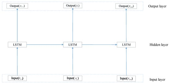
Figure 1. LSTM network.

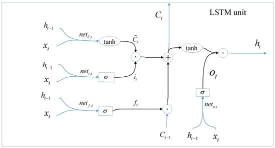
Figure 2. LSTM unit.

The calculation process of LSTM in Figure 2 is as follows:

(1)

Calculate the inputs for three gate units and the candidate cell by Equations (7)–(10):

$$ne{t}_{i,t}=W_i\cdot [x_t,h_{t-1}]+b_i$$

(7)

$$ne{t}_{f,t}=W_f\cdot [x_t,h_{t-1}]+b_f$$

(8)

$$ne{t}_{o,t}=W_o\cdot [x_t,h_{t-1}]+b_o$$

(9)

$$ne{t}_{\tilde{c},t}=W_{\tilde{c}}\cdot [x_t,h_{t-1}]+b_{\tilde{c}}$$

(10)

where $x_t$ represents the inputs at time $t$, and $h_{t-1}$ represents the cell output at time $t-1$. $ne{t}_{i,t}ne{t}_{f,t}ne{t}_{o,t}$$ne{t}_{\tilde{c},t}$ are input gate, forget gate, output gate, and the candidate cell, respectively. $W_i,W_f,W_o,W_{\tilde{c}}$ are the input gate, forget gate, output gate, and weight matrix of the candidate cell, respectively. $b_i,b_f,b_o,b_{\tilde{c}}$ are the bias of input gate, forget gate, output gate, and candidate cell, respectively.

(2)

Calculate the three gate units by Equations (11)–(15):

$$i_t=\sigma (ne{t}_{i,t})$$

(11)

$$f_t=\sigma (ne{t}_{f,t})$$

(12)

$${\tilde{C}}_t=\tan \mathrm{h}(ne{t}_{\tilde{c},t})$$

(13)

$$o_t=\sigma (ne{t}_{o,t})$$

(14)

$$C_t=f_t\cdot C_{t-1}+i_t\cdot {\tilde{C}}_t$$

(15)

where $i_t$, $f_t$, $C_t$, $o_t$, ${\tilde{c}}_t$ represent the input gate at time t, forget gate, unit state, output gate, and candidate cell vector unit output, respectively. $\sigma (\cdot )$ stands for sigmoid activation function and is expressed by Equation (16):

$$\sigma (x)=\frac{1}{1+e^{-x}}$$

(16)

tanh(·) stands for tanh activation function and is expressed by Equation (17):

$$\tan (x)=\frac{e^x-e^{-x}}{e^x+e^{-x}}$$

(17)

(3)

Calculate the output by Equation (18):

$$h_t=o_t\cdot \tan \mathrm{h}(C_t)$$

(18)

where $h_t$ is the unit output at time $t$.

2.2.2. Selection of Hyperparameters

Many parameters for LSTM can affect its accuracy and performance. The selected hyperparameters are a learning rate, the number of units of the hidden layer, and the number of batch size. If the selected learning rate is too small, the convergence will be too slow; otherwise, the cost function will oscillate. The number of units of the hidden layer will influence the effect of fitting. For the number of batch size, if this number is too small, then the training data will be extremely difficult to converge, which will lead to underfitting. If the number is too large, then the required memory will increase significantly. For example, when the number of units of the hidden layer is specified within (1, 100) and the range of the number of batch size is specified within (1, 500), a total of 50,000 combinations will be generated. Thus, to overcome the computational burden, a simple yet reliable algorithm should be utilized to select the optimal combination of parameters for balancing predictive performance and computational efficiency. In this paper, the hyperparameters of LSTM are determined by means of the DE algorithm. DE is a heuristic random search algorithm based on group differences [40]. The objective function of the optimization problem to select hyperparameters is the root mean square error (RMSE), which represents the sum of the squared deviations of the predicted value and the true value calculated by Equation (19):

$$RMSE=\sqrt{\frac{1}{s}{\displaystyle \sum }_{i=1}^s{({\tilde{y}}_i-y_i)}^2}$$

(19)

where ${\tilde{y}}_s$ is the sth predicted value, $y_s$ is the sth true value.

The process of the DE algorithm to select LSTM hyperparameters is shown below:

(1)

Initialization: Initialize the following parameters: length of individual D, number of iterations G, population size NP, crossover rate, and scaling or mutation factor. The population is randomly generated by Equation (20):

$$X_{\omega ,k}=X_{\omega ,k}^L+rand\ast (X_{\omega ,k}^U-X_{\omega ,k}^L)$$

(20)

where $\omega$ = 1, 2, …, NP; $k$ = 1, 2, …D; $X_{\omega ,k}^L$ and $X_{\omega ,k}^U$ are the upper and lower bounds of the k-th dimension, respectively.

(2)

Mutation: Mutation operator is used to generate the mutation vector (H_i) for the individual of the population using Equation (21).

$$H_i(g+1)=X_{r1}(g)+F\ast (X_{r2}(g)-X_{r3}(g))$$

(21)

where $x_{r1}(g)$, $x_{r2}(g)$, $x_{r3}(g)$ are individuals randomly selected from the population, and $r1\ne r2\ne r3$, F is the scaling factor and g represents the g-th generation.

(3)

Crossover: Crossover operation is to randomly select individuals using Equation (22)

$$U_{\omega ,k}(g+1)=\{\begin{array}{cc}{H}_{\omega ,k}(g+1)& if rand(0,1)\le CR\\ X_{\omega ,k}(g)& \mathit{otherwise}\end{array}$$

(22)

where $U_{\omega ,k}$ is the new individual generated in the crossover operation, $CR$ is the crossover rate.

(4)

Selection: In the selection operator as shown in Equation (23), for minimization problems, if the fitness value $f(U_{\omega ,k}(g+1))$ of the trial vector $U_{\omega ,k}(g+1)$ is less than or equal to the fitness value $f(X_{\omega ,k}(g))$ of the target vector $X_{\omega ,k}(g)$, the trial vector will replace the target vector and enter the population. Otherwise, the target vector is still retained.

$$X_{\omega ,k}(g+1)=\{\begin{array}{cc}{U}_{\omega ,k}(g+1)& if f(U_{\omega ,k}(g+1)\le f(X_{\omega ,k}(g))\\ & X_{\omega ,k}(g)\end{array}$$

(23)

The best individual is the three hyperparameters of the LSTM prediction network structure. In this paper, the best set of hyperparameters is selected by comparing the RMSE corresponding to different hyperparameter values generated by training.

2.3. Proposed Prediction Framework

The framework of the proposed prediction algorithm, shown in Figure 3, includes three parts. They are Part A (Data processing), Part B (Hyperparameters optimization), and Part C (Forecasting).

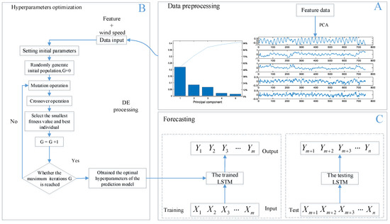
Figure 3. The proposed prediction framework.

In Part A, 11 types of meteorological data (feature data in Part A), such as temperature, humidity, air pressure, and wind level, are dimensionally reduced by PCA. The data processed by the PCA algorithm and historical wind speed data together form the input of Part B. Part B uses the hyperparameters selected by DE to obtain a new LSTM model. Part C first divides the processed data in part A into a training set and a test set, and then applies the LSTM model in part B to forecast wind speed.

2.4. Evaluation Metric of Prediction

In order to evaluate the performance of the proposed model, four different indicators, including RMSE (see Equation (19)), mean absolute error (MAE), mean absolute percentage error (MAPE), and coefficient of determination (denoted by $R^2$), are adopted as evaluation metrics.

(1) MAE

MAE is the average of the absolute error and can reflect the error between the predicted value and the actual value well. The smaller the MAE is, the higher the accuracy the prediction achieves. The formula is as follows.

$$MAE=\frac{1}{s}{\displaystyle \sum }_{i=1}^n|{\tilde{y}}_i-y_i|$$

(24)

(2) MAPE

MAPE represents the ratio between the error and the true value. The smaller the MAPE is, the closer the predicted value is to the true value. The formula is as follows.

$$MAPE=\frac{1}{s}{\displaystyle \sum }_{i=1}^s\frac{|{\tilde{y}}_i-y_i|}{y_i}$$

(25)

(3) Coefficient of determination

The coefficient of determination ($R^2$) is the square of the correlation between predicted values and true values. The range of $R^2$ is specified within [0,1]. The closer $R^2$ is to 1, the more perfect fit the prediction model has. Therefore, $R^2$ can be used as an important indicator. The formula is as follows.

$$R^2=\frac{{\sum }_{i=1}^s{({\tilde{y}}_i-\overline{Y})}^2}{{\sum }_{i=1}^s{(y_i-\overline{Y})}^2}$$

(26)

where $\overline{Y}$ is the mean of the observed value.

3. Case Study

In this section, the description of meteorological data is first introduced. Then, the experimental design and parameter settings are described. Finally, results and analysis are shown to validate the performance of the proposed method.

3.1. Data Description

The meteorological data came from Fuyun Meteorological Station (N 46.59°, E 89.31°) located at Xinjiang province in China [33]. The time span was one month (from 00:00 on the 15th of July, 2018 to 23:00 on the 14th of August). The total length of the sample was 744 with an hourly resolution. The basic information of meteorological factors is listed in Table 1. Hourly wind speed data shown in Figure 4 were divided into a training set (the first 624 points) and a test set (the last 120 points).

Table 1. Basic information of meteorological factors.

Feature Number	Factor	Unit	Min	Max	Mean	Std
1	Air pressure	hpa	902	919.5	909.96	3.42
2	Sea level pressure	hpa	993.9	1017.4	1004.5	4.37
3	Air temperature	°C	10.2	35.3	22.64	5.09
4	Apparent temperature	°C	9.16	32.32	21.74	4.85
5	Extreme wind speed	m/s	1.2	15.65	6.48	3.76
6	Wind level	\	1	6	2.62	1.27
7	Relative humidity	%	10	91	40.88	16.99
8	Minimum relative humidity	%	8	90	38.3	16.28
9	Vapor pressure	hpa	4.3	18.4	10.36	2.41
10	Precipitation	mm	0	0.7	0.00	0.04
11	Horizontal visibility	m	7500	35,000	34,462	2652.5

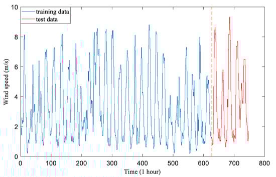
Figure 4. Training set and test set.

3.2. Experimental Design and Parameter Settings

We first used the PCA algorithm to calculate the contribution and cumulative contribution rate of each component as shown in Table 2. It can be seen that as the number of features increased, the correlation became more and more obvious, which means that there was no need to measure all the features. The cumulative contribution rate of the first five principal components was 0.9653. Therefore, these five principal components and wind speed were selected to form the input to the prediction models.

Table 2. Calculation results of each principal component.

Principal Component	Eigenvalues	Contribution Rate	Cumulative Contribution Rate
First	0.2189	0.5238	0.5238
Second	0.0843	0.2017	0.7255
Third	0.0661	0.1582	0.8837
Fourth	0.0203	0.0485	0.9322
Fifth	0.0138	0.0331	0.9653
Sixth	0.0091	0.0217	0.9870
Seventh	0.0027	0.0065	0.9935
Eighth	0.0021	0.0051	1.0
Ninth	0.0003	0.0007	1.0
Tenth	0.0003	0.0006	1.0
Eleventh	0	0	1.0

To validate the prediction performance of the proposed PCA-LSTM method, BPNN-, SVR-, GPR-, and RNN-based methods were selected for comparison. The following three cases were studied:

Case I: LSTM model optimized by DE algorithm and comparisons with BPNN, GPR, RNN, and SVR only using historical wind speed data

Case II: Feature-LSTM model optimized by DE algorithm and comparisons with Feature-BPNN, Feature-GPR, Feature-RNN, and Feature-SVR using all meteorological factors related to wind speed data

Case III: the proposed model and comparisons with PCA-BPNN, PCA-GPR, PCA-RNN, and PCA-SVR using meteorological factors processed by the PCA algorithm.

On the basis of several trials and similar works [40,41], the parameters of the DE algorithm were set as follows: population size NP = 10, number of iterations G = 20, scaling factor F = 0.6, and crossover factor CR = 0.8. For the LSTM network, the range of the learning rate was specified within [0, 1], the range of the number of hidden layer units was within [1, 100], and the range of the batch size was specified within [1, 100]. Table 3 shows parameter settings of LSTM determined by the DE algorithm and other models. Furthermore, the Adam algorithm was adopted to make calculation of the LSTM network more efficient [40]. For SVR and GPR, the results of each run were the same, hence, they ran once. For network-based methods, such as BPNN, LSTM, and RNN, the results obtained by each run were different; these models ran independently for 10 times, and the average was recorded as the final result.

Table 3. Parameter settings.

Model	Parameters	Value	Reason
LSTM Feature-LSTM Proposed Model	Learning rate	0.0047	Obtained by DE
	Hidden unit	68	Obtained by DE
	Batch size	29	Obtained by DE
	Epochs of training	1000	Converged
BPNN Feature-BPNN PCA-BPNN	Hidden unit	10	Common value
	Epochs of training	1000	Converged
SVR Feature-SVR PCA-SVR	Kernel function	Radial Basis Function	A competitive kernel function
	Parameter in Radial Basis Function	1	Common value
GPR Feature-GPR PCA-GPR	Kernel Function	Gaussian Function	A competitive kernel function
	Parameter in Gaussian Function	2	Common value
	Parameter in Gaussian Function	1	Common value
RNN Feature-RNN PCA-RNN	Hidden unit	10	Common value
	Epochs of training	1000	Converged

3.3. Prediction Result Analysis

Case I was to demonstrate the effectiveness of the LSTM model optimized by the DE algorithm compared with the BPNN, GPR, RNN, and SVR models. The forecasting indicators obtained from the above models are shown in Table 4, where the best results for each model are in bold. For the LSTM model, the average values of RMSE, MAE, MAPE, and $R^2$ were 0.3327, 0.2598, 0.1004, and 0.9655, respectively. Compared with other models, the LSTM model optimized by DE performed the best in RMSE, MAE, and $R^2$. In order to more intuitively compare the above five models, the forecasting wind speed and $R^2$ for each model are shown in Figure 5. The coefficient of determination of the LSTM model was the largest. So, the fitting effect was the best and the prediction was the most accurate. To summarize, the LSTM model optimized by the DE algorithm provided better performance than the other four traditional models.

Table 4. Evaluation prediction results in Case I.

Model	Statistical Indicators	RMSE	MAPE	MAE	R2
BPNN	Min	0.8038	0.2022	0.6138	0.6967
	Mean	0.8435	0.2109	0.6344	0.879
	Max	1.029	0.2447	0.721	0.9518
GPR	/	0.8034	0.2054	0.619	0.8688
LSTM	Min	0.3198	0.0930	0.2386	0.9471
	Mean	0.3327	0.1004	0.2598	0.9655
	Max	0.3483	0.1077	0.2753	0.9791
RNN	Min	0.8026	0.0507	0.6188	0.8601
	Mean	0.8044	0.0521	0.6193	0.8666
	Max	0.8075	0.0533	0.6199	0.8723
SVR	/	0.8292	0.1864	0.6099	0.8814

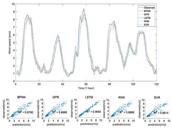
Figure 5. Forecast results in Case I.

In Case II, we used meteorological characteristics related to wind speed as input of the five forecasting models. Table 5 and Figure 6 show the performance metrics of forecasting results achieved by the above five different models. RMSE, MAPE, and MAE of the Feature-LSTM model were 0.1745, 0.0488, and 0.1212, respectively. $R^2$ of the Feature-LSTM was 0.9749, which was slightly smaller than that of Feature-BPNN. Overall, the comprehensive prediction performance of the Feature-LSTM was the best among all the above models. Compared with Case 1, all four indicators improved significantly.

Table 5. Evaluation of prediction results using meteorological characteristics model.

Model	Statistical Indicators	RMSE	MAPE	MAE	R2
Feature-BPNN	Min	0.2425	0.0702	0.1832	0.9650
	Mean	0.3352	0.0975	0.2498	0.9806
	Max	0.4575	0.1418	0.3218	0.9902
Feature-GPR	/	0.1898	0.0535	0.1379	0.9546
Feature-LSTM	Min	0.1577	0.0429	0.1057	0.9592
	Mean	0.1745	0.0488	0.1212	0.9749
	Max	0.1926	0.0535	0.1334	0.9942
Feature-RNN	Min	0.1693	0.0471	0.1232	0.9066
	Mean	0.2077	0.0613	0.1549	0.9648
	Max	0.2613	0.0871	0.1937	0.9997
Feature-SVR	/	0.9976	0.1726	0.5726	0.704

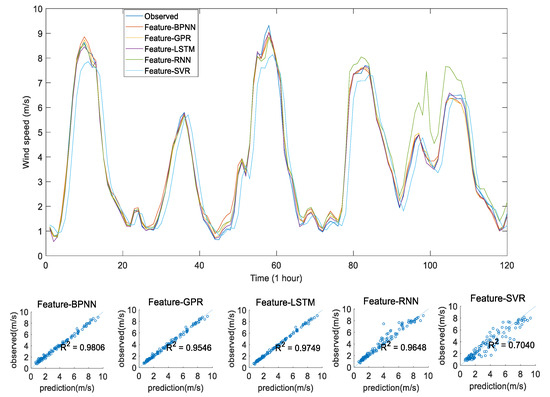
Figure 6. Forecast results in Case II.

The prediction results based on the PCA and LSTM methods of Case III are shown in Figure 7. The figure shows the true values and the predicted values of the five different models. Table 6 is the evaluation index value of each prediction model. Through comparing PCA-LSTM with the PCA-BPNN, PCA-GPR, PCA-RNN, and PCA-SVR models, it can be clearly observed that combined methods had an apparent influence on forecasting performance. From Table 6 and Figure 7, the proposed model outperformed the other four competitors for short-term wind speed forecasting with the smallest mean value of RMSE as 0.1474, MAPE as 0.0382, and MAE as 0.1015, as well as the highest mean value of $R^2$ as 0.9989, making it the best among all prediction models. Therefore, compared with Case I and Case II, the four indicators of the proposed PCA-LSTM method in this article were the best. The PCA-LSTM model achieved superiority in the 15 forecasting models in all cases.

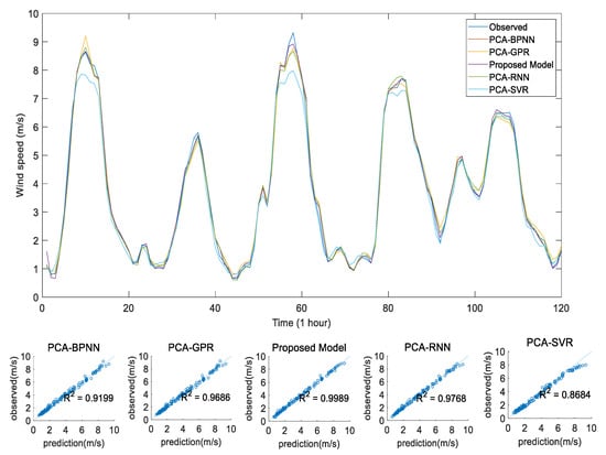
Figure 7. Forecast results in Case III.

Table 6. Evaluation index of prediction results.

Model	Statistical Indicators	RMSE	MAPE	MAE	R2
PCA-BPNN	Min	0.2058	0.0569	0.148	0.8455
	Mean	0.268	0.0793	0.2041	0.9199
	Max	0.4854	0.1155	0.3558	0.9739
PCA-GPR	Mean	0.1706	0.046	0.1231	0.9686
Proposed Model	Min	0.1380	0.0356	0.0958	F0.9988
	Mean	0.1474	0.0382	0.1015	0.9989
	Max	0.1592	0.0415	0.1088	0.9991
PCA-RNN	Min	0.1693	0.0471	0.1232	0.9167
	Mean	0.2077	0.0613	0.1549	0.9768
	Max	0.2613	0.0871	0.1937	0.9897
PCA-SVR	Mean	0.3071	0.0726	0.2218	0.8684

3.4. Discussion

In the above experiments, the BPNN, GPR, LSTM, RNN, and SVR methods were selected in Case I to predict wind speed using only historical wind speed data. Among them, the comprehensive performance of LSTM was the best, which reflects the strong fitting ability of the LSTM model to the nonlinear problem. By comparing Case I with Case II, the use of meteorological characteristics related to wind speed during wind speed prediction can improve the prediction results. In the comparison between Case II and Case III, the PCA algorithm was used to reduce the dimension of meteorological characteristics related to wind speed, and the prediction results were further improved in all prediction models.

4. Conclusions

In this paper, a hybrid PCA and LSTM prediction method is presented. PCA is used to process original meteorological data. LSTM is optimized by the DE algorithm to obtain the best prediction model. Combining PCA and LSTM shows great advantages. The proposed method is applied to predict wind speed and the results prove that the method has strong predictive ability for time series data. Based on the analyses of Cases I–III, the proposed model not only requires less data than other models, but also largely improves the accuracy of forecasting results.

In our future work, hybrid methods using different deep learning models will be considered for time series prediction. In addition, we will improve the PCA method to make it more applicable and efficient.

References

- Dyrholm, M.; Rebollo, A.; Backwell, B.; Aufderheide, B.; Ohlenforst, K. Global Wind Report 2018; Global Wind Energy Council (GWEC): Brussels, Belgium, 2019. [Google Scholar]
- Yang, X.Y.; Zhang, Y.F.; Yang, Y.W.; Lv, W. Deterministic and Probabilistic Wind Power Forecasting Based on Bi-Level Convolutional Neural Network and Particle Swarm Optimization. Appl. Sci. 2019, 9, 1794. [Google Scholar] [CrossRef]
- Zhang, S.H.; Liu, Y.W.; Wang, J.Z.; Wang, C. Research on Combined Model Based on multi-objective optimization and application in wind speed forecast. Appl. Sci. 2019, 9, 423. [Google Scholar] [CrossRef]
- Jaesung, J.; Robert, P.B. Current status and future advances for wind speed and power forecasting. Renew. Sustain. Energy Rev. 2014, 31, 762–777. [Google Scholar]
- Wang, Q.; Wu, H.; Florita, A.; Martinez, C.B.; Hodge, B.M. The value of improved wind power forecasting: Grid flexibility quantification, ramp capability analysis, and impacts of electricity market operation timescales. Appl. Energy 2016, 184, 696–713. [Google Scholar] [CrossRef]
- Chen, N.Y.; Zheng, Q.; Nabney, L.T.; Meng, X.F. Wind power forecasting using Gaussian Processes and Numerical weather prediction. IEEE Trans. Power Syst. 2014, 29, 656–665. [Google Scholar] [CrossRef]
- Piotrowski, P.; Baczyński, D.; Kopyt, M.; Szafranek, K.; Helt, P.; Gulczyński, T. Analysis of forecasted meteorological data (NWP) for efficient spatial forecasting of wind power generation. Electr. Power Syst. Res. 2019, 175, 105891. [Google Scholar] [CrossRef]
- Marta, P.; Pilar, P.; José, R.P. Automatic tuning of Kalman filters by maximum likelihood methods for wind energy forecasting. Appl. Energy 2013, 108, 349–362. [Google Scholar]
- Erdem, E.; Shi, J. ARMA based approaches for forecasting the tuple of wind speed and direction. Appl. Energy 2011, 88, 1405–1414. [Google Scholar] [CrossRef]
- Zhou, J.Y.; Shi, J.; Li, G. Fine tuning support vector machines for short-term wind speed forecasting. Energ. Convers. Manag. 2011, 52, 1990–1998. [Google Scholar] [CrossRef]
- Zhang, C.; Wang, H.K.; Zhao, X.; Liu, T.H.; Zhang, K.J. A Gaussian process regression based hybrid approach for short-term wind speed prediction. Energy Convers. Manag. 2016, 126, 1084–1092. [Google Scholar] [CrossRef]
- Xia, J.; Wu, W.Q.; Huang, B.L.; Li, W.P. Application of a new information priority accumulated grey model with time power to predict short-term wind turbine capacity. J. Clean. Prod. 2020, 244, 118573. [Google Scholar] [CrossRef]
- Cassiola, F.; Burlando, M. Wind speed and wind energy forecast through Kalman filtering of Numerical Weather Prediction model output. Appl. Energy 2012, 99, 154–166. [Google Scholar] [CrossRef]
- Singh, S.N.; Mohapatra, A. Repeated wavelet transform based ARIMA model for very short-term wind speed. Renew. Energy 2019, 136, 758–768. [Google Scholar]
- Rjoub, G.; Bentahar, J.; Wahab, O.A.; Bataineh, A. Deep Smart Scheduling: A Deep Learning Approach for Automated Big Data Scheduling Over the Cloud. In Proceedings of the 2019 7th International Conference on Future Internet of Things and Cloud (FiCloud), Istanbul, Turkey, 26–28 August 2019; pp. 189–196. [Google Scholar]
- Wahab, O.A.; Bentahar, J.; Otrok, H.; Mourad, A. Resource-Aware Detection and Defense System Against Multi-Type Attacks in the Cloud: Repeated Bayesian Stackelberg Game. IEEE Trans. Dependable Secur. Comput. 2019, 2907946. [Google Scholar] [CrossRef]
- Wahab, O.A.; Cohen, R.; Bentahar, J.; Otrok, H.; Mourad, A.; Rjoub, G. An endorsement-based trust bootstrapping approach for newcomer cloud services. Inf. Sci. 2020, 527, 159–175. [Google Scholar] [CrossRef]
- Sarker, I.H.; Kayes, A.S.M.; Watters, P. Effectiveness Analysis of Machine Learning Classification Models for Predicting Personalized Context-Aware Smartphone Usage. J. Big Data 2019, 6, 57. [Google Scholar] [CrossRef]
- Zameer, A.; Khan, A.; Javed, S.G. Machine Learning based short term wind power prediction using a hybrid learning model. Comput. Electr. Eng. 2015, 45, 122–133. [Google Scholar]
- Heinermann, J.; Kramer, O. Machine learning ensembles for wind power prediction. Renew. Energy 2016, 89, 671–679. [Google Scholar] [CrossRef]
- Treiber, N.A.; Heinermann, J.; Kramer, O. Wind power prediction with Machine Learning. Comput. Sustain. 2016, 645, 13–29. [Google Scholar]
- Hu, Y.L.; Chen, L. A nonlinear hybrid wind speed forecasting model using LSTM network, hysteretic ELM and Differential Evolution algorithm. Energy Convers. Manag. 2018, 173, 123–142. [Google Scholar] [CrossRef]
- Zhang, Y.G.; Chen, B.; Zhao, Y.; Pan, G. Wind Speed Prediction of IPSO-BP Neural Network Based on Lorenz Disturbance. IEEE Access 2018, 6, 53168–53179. [Google Scholar] [CrossRef]
- Liu, H.; Mi, X.W.; Li, Y.F.; Duan, Z.; Xu, Y.N. Smart wind speed deep learning based multi-step forecasting model using singular spectrum analysis, convolutional gated recurrent unit network and support vector regression. Renew. Energy 2019, 143, 842–854. [Google Scholar] [CrossRef]
- Ma, T.; Wang, C.; Wang, J.Z.; Cheng, J.J.; Chen, X.Y. Particle-swarm optimization of ensemble neural network with negative correlation learning for forecasting short-term wind speed of wind farms in western China. Inf. Sci. 2019, 505, 157–182. [Google Scholar] [CrossRef]
- Pei, S.Q.; Qin, H.; Zhang, Z.D.; Yao, L.Q.; Wang, Y.Q.; Wang, C.; Liu, Y.Q.; Jiang, Z.Q.; Zhou, J.Z.; Yi, T.L. Wind speed prediction method based on Empirical Wavelet Transform and New Cell Update Long Short-Term Memory network. Energy Convers. Manag. 2019, 196, 779–792. [Google Scholar] [CrossRef]
- Zhang, Z.D.; Ye, L.; Qin, H.; Liu, Y.Q.; Wang, C.; Yu, X.; Yin, X.L.; Li, J. Wind speed prediction method using Shared Weight Long Short-Term Memory Network and Gaussian Process Regression. Appl. Energy 2019, 247, 270–284. [Google Scholar] [CrossRef]
- Khosravi, A.; Machado, L.; Nunes, R.O. Time-series prediction of wind speed using machine learning algorithms: A case study Osorio wind farm, Brazil. Appl. Energy 2018, 224, 550–566. [Google Scholar] [CrossRef]
- Ronay, A.; Olga, F.; Enrico, Z. Two machine learning approaches for short-term wind speed time-series prediction. IEEE Trans. Neural Netw. Learn. Syst. 2015, 27, 1734–1747. [Google Scholar]
- Hong, Y.Y.; Paulo, P.; Rioflorido, C.L. A hybrid deep learning-based neural network for 24-h ahead wind power forecasting. Appl. Energy 2019, 250, 530–539. [Google Scholar] [CrossRef]
- Kumar, P.S.; Lopez, D. Feature Selection used for Wind Speed Forecasting with Data Driven Approaches. Res. J. Appl. Sci. Eng. Technol. 2015, 8, 921–926. [Google Scholar]
- Fan, S.; Liao, J.R.; Yokoyama, R.; Chen, L.N.; Lee, W.J. Forecasting the Wind Generation Using a Two-Stage Network Based on Meteorological Information. IEEE. Trans. Energy Conver. 2009, 24, 474–482. [Google Scholar] [CrossRef]
- Zhang, Z.D.; Qin, H.; Liu, Y.Q.; Wang, Y.Q.; Yao, L.Q.; Li, Q.Q.; Li, J.; Pei, S.Q. Long Short-Term Memory Network based on Neighborhood Gates for processing complex causality in wind speed prediction. Energy Convers. Manag. 2019, 192, 37–51. [Google Scholar] [CrossRef]
- Zhang, Y.G.; Zhang, C.H.; Zhao, Y.; Gao, S. Wind speed prediction with RBF neural network based on PCA and ICA. J. Electr. Eng. 2018, 69, 148–155. [Google Scholar] [CrossRef]
- Zhang, Y.G.; Chen, B.; Pan, G.F.; Zhao, Y. A novel hybrid model based on VMD-WT and PCA-BP-RBF neural network for short-term wind speed forecasting. Energy Convers. Manag. 2019, 195, 180–197. [Google Scholar] [CrossRef]
- Sarker, I.H.; Abushark, Y.B.; Khan, A.I. ContextPCA: Predicting Context-Aware Smartphone Apps Usage based on Machine Learning Techniques. Symmetry 2020, 12, 499. [Google Scholar] [CrossRef]
- Gupta, V.; Mittal, M. KNN and PCA classifier with Autoregressive modelling during different ECG signal interpretation. Procedia. Comput. 2017, 125, 18–24. [Google Scholar] [CrossRef]
- Hochreiter, S.; Schmidhuber, J. Long short-term memory. Neural. Comput. 1997, 9, 1735–1780. [Google Scholar] [CrossRef]
- Liu, Y.; Guan, L.; Hou, C.; Han, H.; Liu, Z.J.; Sun, Y.; Zheng, M.H. Wind Power Short-Term Prediction Based on LSTM and Discrete Wavelet Transform. Appl. Sci. 2019, 9, 1108. [Google Scholar] [CrossRef]
- Wang, L.; Zeng, Y.; Chen, T. Back propagation neural network with adaptive differential evolution algorithm for time series forecasting. Expert Syst. Appl. 2015, 42, 855–863. [Google Scholar] [CrossRef]
- Cui, L.Z.; Huang, Q.L.; Li, G.H.; Yang, S.; Ming, Z.; Wen, Z.K.; Lu, N.; Lu, J. Differential Evolution Algorithm with Tracking Mechanism and Backtracking Mechanism. IEEE Access 2018, 6, 44252–44267. [Google Scholar] [CrossRef]
© 2020 by the authors. Licensee MDPI, Basel, Switzerland. This article is an open access article distributed under the terms and conditions of the Creative Commons Attribution (CC BY) license (http://creativecommons.org/licenses/by/4.0/).