Estimation of Cyclic Demand in Metallic Yielding Dampers Installed on Frame Structures

Featured Application

Assessment and design of hysteric dampers considering the impulsive effects of earthquakes.

Abstract

The efficacy of hysteretic dampers can be formulated as the number or equivalent inelastic cycles, or the ratio of normalised dissipated energy to displacement ductility. This parameter is used in the design of framed structures with supplemental dampers and it is strongly influenced by the impulsive effects of earthquakes and other structural parameters. This paper presents an estimate of the cyclic demand of dampers installed in reinforced concrete frames, based on nonlinear time history analyses. Statistical analyses of the results are used to highlight relevant parameters and calibrate a predictive formula and upper-bound design values. The collapse pattern of the frames seems to have no effect on the efficacy of the dampers; thus, the seismological parameters that describe impulsivity should drive the design of hysteric dampers.

1. Introduction

Metallic yielding dampers are a cost-effective technology for passive seismic control of the vibration of structures. In buildings, these types of dampers are generally installed into new or retrofitted framed structures to ensure reliable seismic performance through inelastic energy dissipation. Unlike velocity dependent dampers such as viscous and viscoelastic or other design strategies [1,2], the force output and amount of dissipated energy does not depend on the loading rate [3], but rather on the magnitude of displacement and on accumulated displacement. Maholtra [4] observed that pulse-like ground motions have dramatic effects on structural response, such as reduced apparent flexibility of high-rise and base-isolated buildings, increased base shear and inter-storey drifts in high-rise buildings, reduced effectiveness of supplemental damping, and increased ductility demand.

Consequently, near-fault ground motions can expose aseismic devices to critical working conditions and a significant reduction in their efficacy. This issue has been studied in base isolated systems [5,6,7,8,9,10], raising concerns about the viability of base isolation and leading to specific design provisions in the near-fault to accommodate lateral deformation and optimise supplemental damping. The effects of near-fault seismicity on the seismic performance of aseismic dampers has also been addressed. Although dampers still provide seismic protection compared to bare frames in the near-fault [11], it has been shown that earthquake impulsive effects lead to the need for higher yield strength and to a decrease in the available local ductility in the dampers [12]. This results in lower energy dissipation capacity and requires specific design considerations [13,14,15,16,17]. The number of equivalent cycles of the hysteretic dampers is also relevant to fatigue issues related to heating due to the rate of energy dissipation.

Near-fault records are characterised by shorter durations and tend to produce less inelastic cycles than far-field records. In the case of hysteretic dampers, energy dissipation occurs due to metallic yielding and it is strongly related to cumulative inelastic deformation or cyclic demand in the damper. One approach to tackle cyclic demand is by considering the relationship between dissipated energy at a maximum or target displacement.

Zahran and Hall [18] investigated the response of elastic-perfectly plastic single-degree-of-freedom (SDOF) systems and noted that structures can absorb more or less energy despite experiencing the same peak displacement. Because energy dissipation must be related to cyclic or cumulative demand, they formulated the concept of equivalent number of yield cycles N. This is defined in Equation (1) and shown in Figure 1, as the ratio of the total energy, E_H that is dissipated by yielding within the structure when subjected to the ground motion of an earthquake to the area under the monotonic load-displacement curve at the same maximum displacement, δ_m, experienced during the vibration.

$$N=\frac{E_H}{Q_y\left({\delta }_m-{\delta }_y\right)}$$

(1)

Zahran and Hall’s results show that the equivalent number of yield cycles N is a useful parameter to define the severity or damage potential of the ground motion. It is influenced by (i) the characteristics of the ground motion: N increases with duration and tends to decrease for near-field records; (ii) the fundamental period: N increases for structures in the 0.2–2 Hz range; and (iii) ductility: N greatly increases as the displacement ductility increases. The number of equivalent cycles N is sometimes termed as n_eq in the literature.

Akiyama [19,20,21] addressed the correspondence between the cumulative inelastic deformation ratio, η defined in Equation (2) (i.e., dissipated hysteretic energy normalised to the yield force Q_y and displacement δ_y) and the inelastic deformation ratio μ defined in Equation (3) (i.e., plastic deformation normalised to δ_y) through numerical analyses with elastic-plastic systems with 5 degrees of freedom. Equation (4) shows that N and the ratio η/μ take the same value. The ratio η/μ is also referred to as the “efficacy” of the structural element.

$$\mathsf{\eta }=\frac{E_H}{Q_y{\delta }_y}$$

(2)

$$\mathsf{\mu }=\frac{{\delta }_m-{\delta }_y}{{\delta }_y}$$

(3)

$$N=\frac{E_H}{Q_y\left({\delta }_m-{\delta }_y\right)}=\frac{\mathsf{\eta }}{\mathsf{\mu }}$$

(4)

Akiyama highlighted that, if known in advance, the ratio η/μ allows us to estimate the maximum expected displacement for a certain amount of dissipated energy demand. Regardless of any other parameters, he proposed an approximate design value of η/μ = 2 for bare elastic-perfectly plastic frames with no strength deterioration. This expression suggests that the efficacy of the structure (in terms of the relationship between dissipated energy and maximum displacement) can be predicted for a certain lateral carrying system under the design earthquake.

Akiyama also proposed design values [19,20,21] of the ratio η/μ in Equation (5) for flexible-stiff mixed frame multi-storey systems, consisting of (i) a flexible part or frame element able to restrain the lateral deformations within the elastic range for the maximum drift expected under the seismic loading (Figure 2a), and (ii) a stiff part or energy absorbing elements (namely, dampers) with high elastic rigidity and large deformation capacity (Figure 2b). Figure 2c represents the behaviour of the mixed system. Because of the added complexity of the mixed multi-storey system, a parametric study was used to focus on structures with predetermined lateral stiffness and strength distributions, and changing the parameter r_q = _fQ_m/_sQ_y, that is, the ratio of the maximum force in the flexible part, _fQ_m, by the yield strength of the stiff part, _sQ_y. From the results of these studies, it can be concluded from Equation (5) that as r_q increases, the number of equivalent yield cycles in the dampers increases, leading to the following relationship:

$$N=\frac{\mathsf{\eta }}{\mathsf{\mu }}=\{\begin{array}{ll}4+r_q& r_q\le 1\\ 8~12& r_q>1\end{array}$$

(5)

Malhotra [22] proposed a cyclic demand spectra that specifies the number of cycles for which the seismic load must be resisted by a structure, and noted that both the amplitude and the number of cycles should be considered in assessing the damage potential of ground motions. Malhotra’s alternative definition of the number of cycles N_cy is based on dividing cumulative damage by the damage caused by a full cycle of largest amplitude u_max. The Coffin–Manson law was used for damage and damage is accumulated by the Miner’s rule. The number of equivalent cycles of amplitude u_max that cause the same damage to the structure as the entire deformation history of n half-cycles of amplitude u_i is given by Equation (6), where c is a structural damage parameter that requires experimental calibration. Cyclic demand spectra are site-specific, so they contain all uncertainties related to the ground motion and yield level, so, the only variable is the fundamental period. Exponent c must account for the rest of the structural characteristics. Based on the definition of the number of cycles in Equation (6), three cyclic spectral parameters N_A, N_V, N_D are introduced to characterise cyclic response, depending on whether the structural response is to be governed by acceleration, velocity or displacement histories. The assumption behind this reasoning is that cyclic response depends primarily on the stiffness of the system. It was found that N_A > N_V > N_D so a stiff structure is likely to experience a larger number of cycles than a flexible structure. Relative stiffness was measured by the ratio of the fundamental period to the earthquake central period.

$$N_{cy}=\frac{1}{2}{\displaystyle \sum }_{i=1}^{2n}{\left(\frac{u_i}{u_{max}}\right)}^c$$

(6)

Kunnath and Chai [23] claimed that the estimation of cyclic deformation demand resulting from earthquake load is crucial if the damage of the system needs to be evaluated, and they produced a cyclic demand spectra to assess the number of full inelastic cycles, N_f. The expression for N_f in Equation (7) includes an energy shape factor α_h that depends on both the ductility and the shape of the hysteresis loops. Structural properties such as Q_y and δ_y are eliminated from Equation (7) with a focus on seismic design by introducing the relationships between fundamental period T, displacement ductility μ, and the seismic response modification factor R. As a result, the number of inelastic cycles in a SDOF can be calculated with Equation (8) as a function of the hysteretic energy E_H, the mass m, the displacement ductility (μ + 1) = δ_max/δ_y, the force reduction factor R, fundamental period T, energy shape factor α_h, and spectral acceleration S_a. Use of Equation (8) implies prior knowledge of several variables including ground motion parameters, structural parameters, and target ductility. For each specific structural system, a series of empirical expressions can be calibrated to relate E_H, R, α_h, and μ, to arrive at simple expressions with only one variable.

$$N_f=\frac{E_H}{4{\alpha }_h{Q}_y{\delta }_y\left(\mu +1\right)}$$

(7)

$$N_f=\left(\frac{E_H}{m}\right)\frac{{\pi }^2}{\left(\mu +1\right){\alpha }_h}{\left(\frac{R}{T{S}_a}\right)}^2$$

(8)

Manfredi [24] underlined that the equivalent number of yield cycles varies largely depending on the characteristics of the ground motion, with values varying from 1 for impulsive records and up to 40 for long-duration records. Statistical regressions of nonlinear time history analyses using two components of 122 European ground motion records revealed that the equivalent number of yield cycles can be predicted with the exponential type expression in Equation (9). It was found that (i) the elastic behaviour is well described by the ratio τ of the fundamental period, T, to the corner period within short and medium/long periods in the spectrum, T_G, where the spectrum changes from the constant acceleration segment to the constant velocity segment; (ii) the plastic behaviour is described with the strength reduction factor R; and (iii) the seismological parameter with the highest correlation factor is the dimensionless parameter I_d = 2g·I_A/(π·PGA·PGV), where I_A is the Arias intensity, PGA is peak ground acceleration, and PGV is peak ground velocity.

Further research by Manfredi et al. [25] has shown that I_d correlates well to the equivalent number of yield cycles N both in the vicinity of the source and far from it. Using regression analyses with 128 near-fault and 122 far-field records, sets of parameters in Equation (9) were calibrated in order to assess the number of yield cycles experienced by a SDOF structure in the far-field and in the near-fault. They observed that N tends to increase with I_d and that I_d tends to increase with the distance to the earthquake source. These observations led them to conclude that the relative importance of the cyclic demand grows at higher distances from the fault, while structural response is governed by peak demand in the near-fault. Using this equation requires calibration of the regression parameters C, $\chi$, $\phi$, and $\kappa$.

$$N=1+C·{\tau }^{\chi }·{\left(R-1\right)}^{\phi }·I_d^{\kappa }$$

(9)

It can be deduced from Equations (6)–(9) that (i) accurate predictions of the number of inelastic cycles requires calibration of parameters for each specific structural system or hysteretic behaviour, (ii) all equations recognise the influence of the yield level (either via R or μ), and (iii) impulsive near-fault ground motions has been found to significantly reduce the number of inelastic cycles. This last point is of paramount importance in the design of structures with hysteretic dampers in the near-fault. Because the response of hysteric dampers is displacement dependent, the decrease in the number of yield cycles necessarily reduces the efficacy of the dampers.

The purpose of this investigation is to highlight the relevant parameters to predict the equivalent number of yield cycles (η/μ) of hysteretic dampers installed in reinforced frames within the framework of performance-based seismic design, with explicit consideration of near-fault effects. To this end, this paper analyses the seismic response of twelve representative reinforced concrete (RC) frames equipped with hysteretic dampers in a region with medium to high seismicity in Europe. The numerical models account for three building heights (3, 6, 9 stories), the collapse pattern of the bare RC frames (with or without capacity design), and two setups of hysteretic dampers (designed for near-fault or far-field seismicity).

2. Materials and Methods

The methodology is based on nonlinear time history analyses of 12 numerical models of RC frames equipped with hysteretic dampers. These analyses were performed using a research code to implement the stiffness method. The solver uses the well-known Newmark-beta method. The nonlinear behaviour was accounted for using a hysteretic model for RC sections with normal cyclic degradation, and a hysteretic model for yielding dampers accounting for the Bauschinger effect. The response of each model was analysed under two seismic scenarios, far-field (FF) or near-fault (NF). The main differences among the models were: (i) building height, 3, 6, and 9 storeys, and (ii) capacity design (CD), that is, enforcing or not of capacity design rules to achieve a weak beam strong column lateral collapse pattern in the RC frame. Capacity design rules to achieve a weak-beam strong-column lateral collapse pattern consist of a ratio of ultimate moment capacity of columns to beam that is larger than 1.71 [21].

Table 1. Summary of buildings models.

Storeys	Far-Field Seismicity	Near-Fault Seismicity
3	3FF-3FFCD	3NF-3NFCD
6	6FF-6FFCD	6NF-6NFCD
9	9FF-9FFCD	9NF-9NFCD

shows a summary of the 12 models, where each model is labelled as follows, number of storeys-seismic scenario-capacity design (e.g., 3 storeys under near-fault and designed without capacity rules would be 3NF. The same, with capacity rules would be 3NFCD)

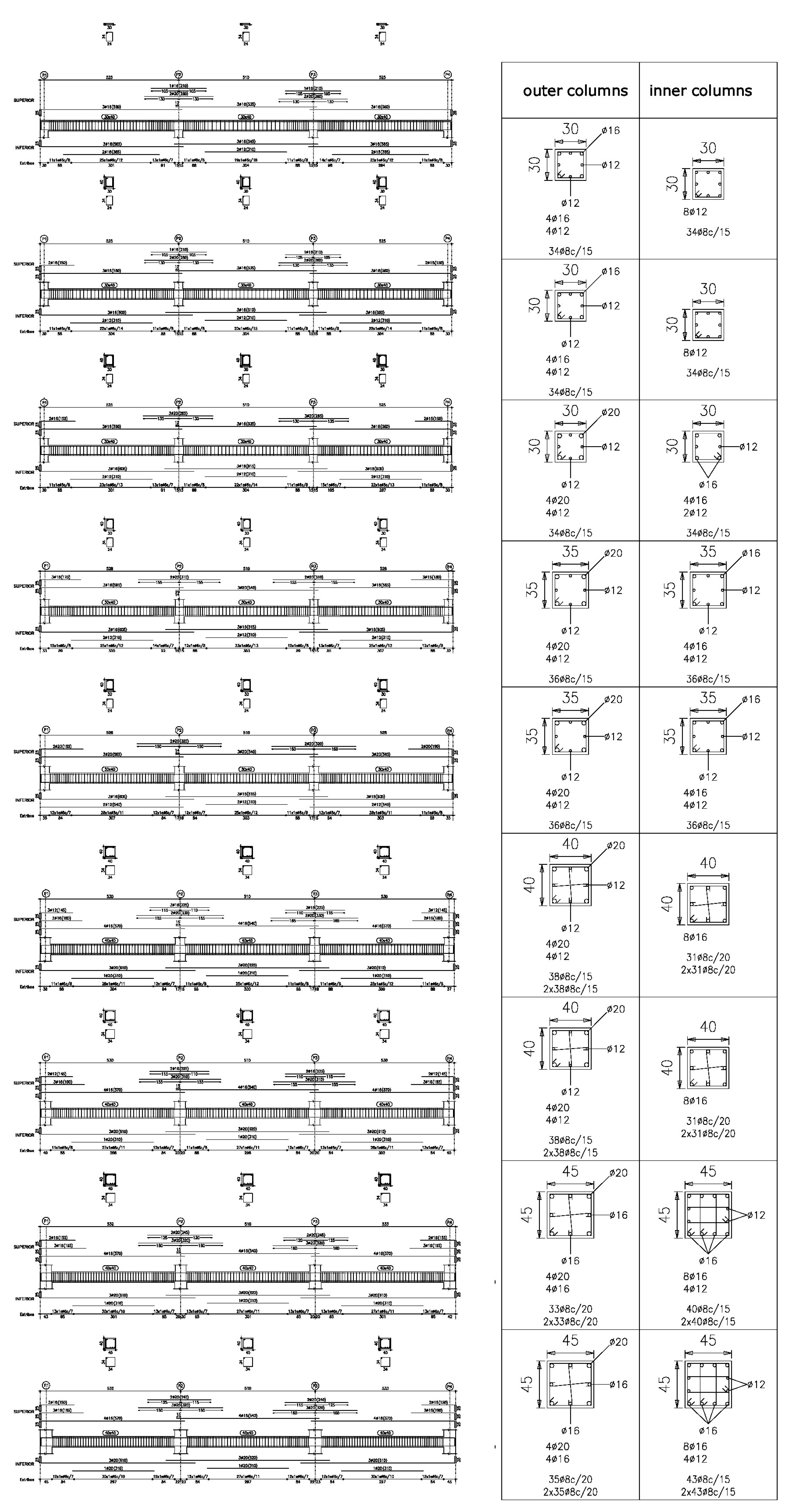
2.1. Design of Prototype Structures

Representative frames were extracted from 3, 6, and 9 storey prototype residential buildings with three 5.1 m bays and storey heights of 3.5 m in the lower floor and 3.1 m for the rest of the storeys. Figure A1, Figure A2 and Figure A3 in Appendix A show the dimensions and reinforcement of the frame elements. RC frames were designed to the limit states, with concrete C25/30 and steel B500S following the Eurocode 8 conventional force-based modal response spectrum analysis, with design ground acceleration a_g = 0.23 g, soil type C and a behaviour factor q = 3. The frames lateral behaviour is characterised by the parameters in

Table 2. Properties of reinforced concrete (RC) frames at floor level: lateral stiffness, yield displacement.

MODEL	9FF, 9FFCD, 9NF, 9NFCD		6FF, 6FFCD, 6NF, 6NFCD		3FF, 3FFCD, 3NF, 3NFCD
Storey	fk (kN/cm)	fδy (cm)	fk (kN/cm)	fδy(cm)	fk (kN/cm)	fδy (cm)
9	53.25	2.86
8	48.52	3.05
7	49.90	2.95
6	63.19	2.91	56.82	2.94
5	65.15	2.87	52.70	2.88
4	79.19	2.86	66.51	2.83
3	78.71	2.83	65.95	2.85	56.43	3.15
2	86.16	2.96	75.13	2.89	53.48	2.73
1	124.41	2.58	96.43	2.68	58.42	3.42

, that is, the storey lateral stiffness _fk, and the storey lateral yield displacement _fδ_y.

Hysteretic dampers in the RC structures are designed so that the RC frame remains elastic under the action of the design earthquake and damage concentrates on the dampers. This is achieved by applying an energy-based method [17] that spreads damage evenly in the dampers along the height of the building. In this procedure, the design earthquake is characterised in terms of a bilinear velocity spectrum with equivalent velocity V_E = 112.7 cm/s and V_D = 72 cm/s, and a number of seismological parameters: the initial period of the medium period range T_NH, the main period of the ground motion is T_G, the dimensionless parameter I_d, and the exponential regression parameters c₁ and c₂ as formulated by Manfredi et al. [25]. These values are: (i) far-field seismicity c₁ = 0.18; c₂ = 0.60; I_d = 10, T_NH = 0.16 s; T_G = 0.13 s, and (ii) near-fault seismicity c₁ = 0.23; c₂ = 0.40; I_d = 4; T_NH = 0.08 s; T_G = 0.07. The results of the hysteretic damper design for the prototype are summarised in

Table 3. Properties of hysteretic dampers at floor level: lateral stiffness, yield displacement.

MODEL	9FF,9FFCD		9NF,9NFCD		6FF,6FFCD		6NF,6NFCD		3FF,3FFCD		3NF,3NFCD
	sk	sδy	sk	sδy	sk	sδy	sk	sδy	sk	sδy	sk	sδy
9	764	0.22	869	0.23
8	696	0.38	792	0.38
7	716	0.44	81	0.44
6	906	0.38	1032	0.39	611	0.26	745	0.27
5	934	0.40	1064	0.40	566	0.44	691	0.44
4	1136	0.35	1293	0.35	715	0.42	872	0.42
3	1129	0.37	11,284	0.38	709	0.47	865	0.48	777	0.23	1193	0.13
2	1236	0.37	1407	0.37	808	0.46	985	0.46	737	0.37	1131	0.22
1	1784	0.28	1784	0.29	1036	0.40	1268	0.41	805	0.40	1235	0.24

, which shows the lateral stiffness _sk and lateral yield displacement _sδ_y of the dampers at each storey level.

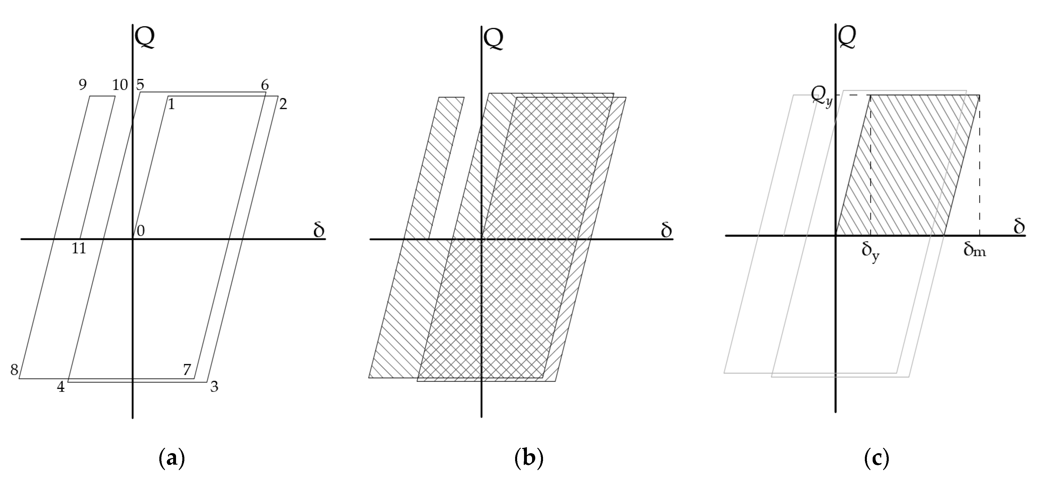
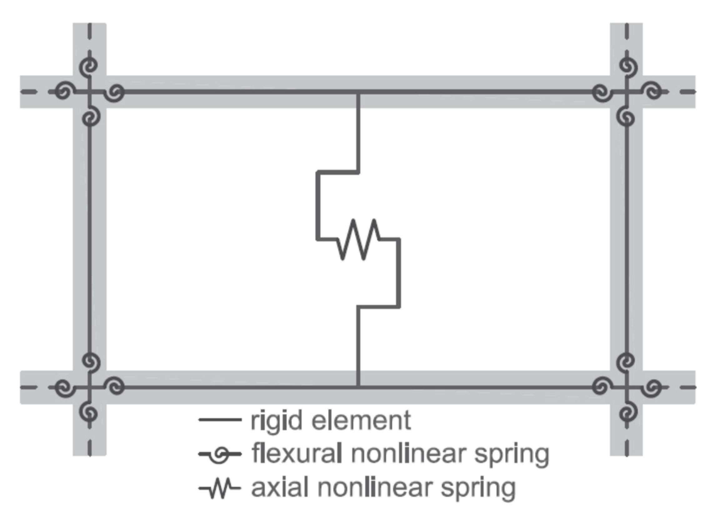
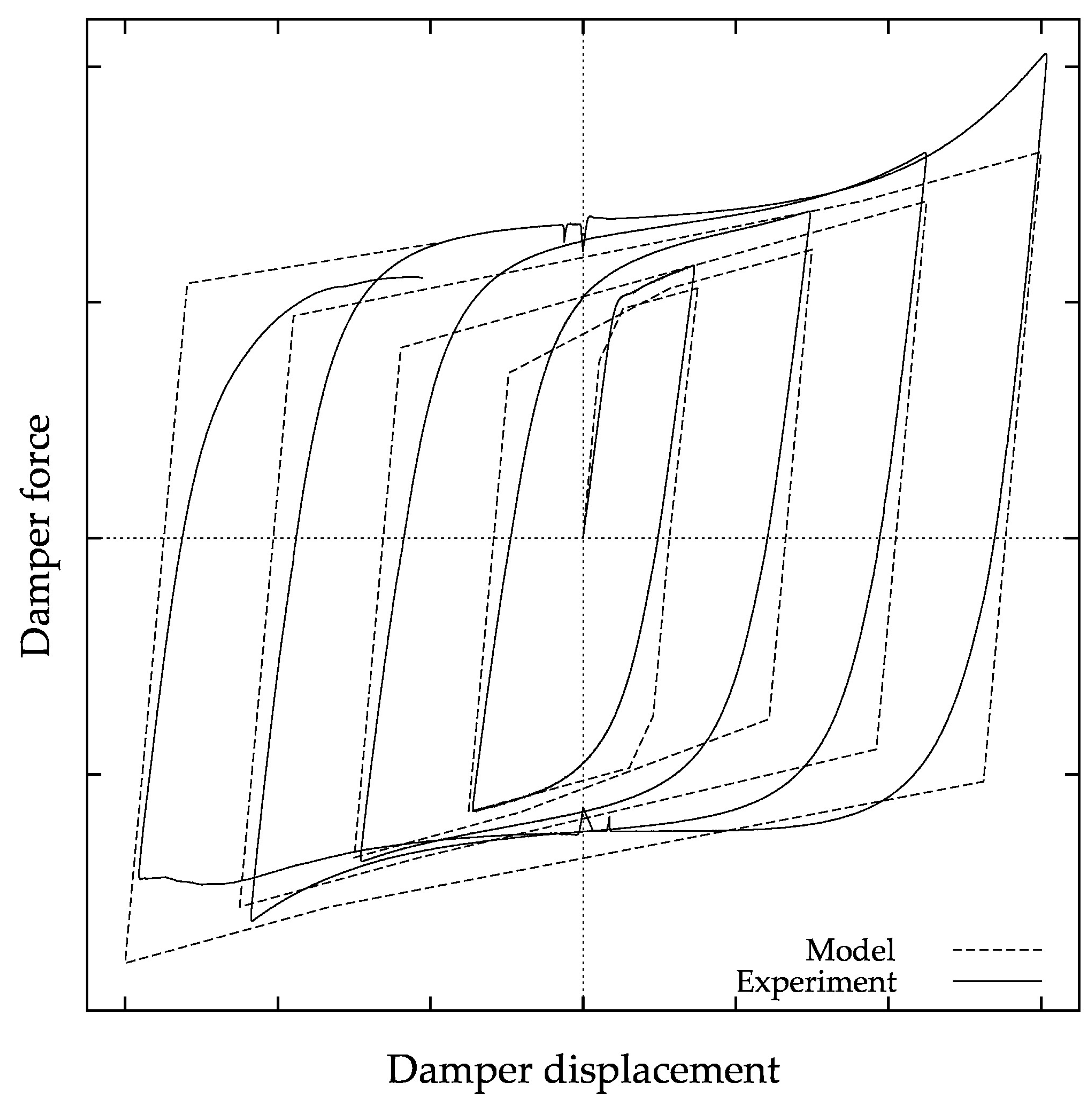
2.2. Numerical Models and Analysis

The RC frames with dampers were modelled as two nonlinear springs connected in parallel with lumped masses at each storey level as shown in Figure 3. Beams and columns in the frame (referred to as flexible elements) are idealised as rigid bars connected by rotational springs or hinges. The nonlinear behaviour of the hinges is given by elastic-perfectly plastic envelopes that are derived from their cross-section dimensions and reinforcement. Four parameters control the cyclic behaviour of the hinges to model the effects of pinching (HS = 0.50), stiffness degradation (HC = 2.00), and strength degradation (HBE = 0.10 and HBD = 0.10) in RC [26,27]. These parameters correspond to normal degradation of reinforced concrete elements. Hysteretic dampers are referred to as stiff elements, and their nonlinear load-deformation behaviour is idealised by a trilinear envelope proportional to the elastic stiffness _sk, and by two parameters (α = 0.66, β = 0.61) that account for the Bauschinger effect in steel. Damper properties are taken from available component testing [28]. An example of the hysteretic model of the dampers is depicted in Figure A4, which shows the nonlinear behaviour of a damper under incremental cyclic displacement.

Seismic action is represented by selecting two sets of ground motion records from the European Strong Motion Database [29]. One set includes 22 far-field records in

Table A2. Properties of ground motion records in the far fault set.

Code	Event	Station	Epic (km)	Local Geology	PGA (m/s2)	PGV (cm/s)	Id	TNH (s)	TG (s)
000948	Sicilia-Orientale	Catania-Piana	24	Soft Soil	2.483	9.86	5.95	0.22	0.2
001257	Izmit	Yarimca-Petkim	20	Soft Soil	2.903	52.68	6.21	0.979	0.84
000123	Friuli (aft)	Forgaria-Cornio	15	Stiff Soil	1.286	8.98	6.23	0.485	0.25
000159	Friuli (aft)	Forgaria-Cornio	7	Stiff Soil	2.365	10.85	6.57	0.347	0.36
000055	Friuli	Tolmezzo-Diga	23	Rock	3.499	20.99	6.79	0.324	0.32
000139	Friuli (aft)	Breginj-Fabri IGLI	25	Stiff Soil	1.558	10.00	7.37	0.423	0.14
000230	Montenegro (aft)	Budva-PTT	8	Stiff Soil	1.172	18.98	7.57	0.683	0.71
000333	Alkion	Korinthos-OTE	20	Soft Soil	2.257	22.45	7.88	0.631	0.5
000134	Friuli (aft)	Forgaria-Cornio	14	Stiff Soil	2.586	9.05	7.92	0.241	0.21
000199	Montenegro	Bar-Skupstina	16	Stiff Soil	3.68	42.5	7.93	1.051	0.96
000229	Montenegro (aft)	Petrovac-Rivijera	17	Stiff Soil	1.708	11.25	8.85	0.176	0.13
000067	Friuli (aft)	Forgaria-Cornio	4	Stiff Soil	1.836	11.46	8.94	0.392	0.39
000074	Gazli	Karakyr Point	11	Vsoft Soil	6.038	51.21	9.61	0.371	0.24
000187	Tabas	Tabas	57	Stiff Soil	9.084	84.36	9.75	0.429	0.33
00197	Montenegro	Ulcinj-H Olimpic	24	Stiff Soil	2.88	38.56	10.41	0.896	0.79
001249	Izmit	Ambarli-Termik	113	Vsoft Soil	2.58	22.11	10.5	0.767	0.82
000290	Campano Lucano	Sturno	32	Rock	2.121	33.52	11.45	0.867	0.49
001703	Duzce	Duzce-Meteoroloji	8	Soft Soil	3.699	35.8	12.15	0.466	0.45
000200	Montenegro	Hercegnovi Novi	65	Rock	2.197	13.75	15.22	0.454	0.37
000196	Montenegro	Petrovac-H Oliva	25	Stiff Soil	4.453	39.16	16.21	0.57	0.46
000182	Tabas	Dayhook	12	Rock	3.316	18.4	16.47	0.196	0.24
002015	Kefallinia	Argostoli-OTE	9	Stiff Soil	1.788	4.96	21.62	0.158	0.16

, and the other set includes other 22 near-fault or pulse-like records in

Table A1. Properties of ground motion in the near-fault set.

Code	Event	Station	Epic (km)	Local Geology	PGA (m/s2)	PGV (cm/s)	Id	TNH (s)	TG (s)
000228	Montenegro	Bar-Skupstina Opstine	33	Stiff Soil	4.985	15.33	1.98	0.516	0.51
000535	Erzincan	Erzincan-Meteorologij	13	Stiff Soil	3.814	101.4	2.54	1.874	1.04
001896	Timfristos	Karpenisi-Prefecture	8	Rock	2.846	7.47	2.56	0.143	0.12
000042	Ionian	Lefkada-OTE	15	Soft Soil	5.146	57.17	2.88	0.663	0.53
001895	Timfristos	Karpenisi-Prefecture	9	Rock	3.089	10.6	2.97	0.079	0.07
000420	Kalamata (aft)	Kalamata-OTE	3	Stiff Soil	2.355	22.03	3.39	0.43	0.4
000419	Kalamata (aft)	Kalamata-Prefecture	1	Stiff Soil	3.275	25.97	3.48	0.476	0.42
000122	Friuli (aft)	Buia	9	Soft Soil	2.261	21.56	3.5	0.598	0.73
000126	Friuli (aft)	Breginj-Fabrika IGLI	21	Stiff Soil	4.647	27.43	3.58	0.3	0.22
000158	Ardal	Naghan 1	7	Rock	8.907	56.85	4.01	0.214	0.12
001714	Ano Liosia	Athens-Sepolia	14	Stiff Soil	2.384	17.91	4.3	0.297	0.16
000146	Friuli (aft)	Forgaria-Cornio	14	Stiff Soil	3.395	22.81	4.34	0.353	0.24
000147	Friuli (aft)	San Rocco	14	Stiff Soil	1.384	11.93	4.55	0.461	0.26
000414	Kalamata	Kalamata-OTE Build	11	Stiff Soil	2.354	31.66	4.63	0.476	0.41
000558	Pyrgos	Pyrgos-AgriBank	10	Soft Soil	1.424	9.29	4.8	0.25	0.21
001313	Ano Liosia	Athens 3	16	Stiff Soil	2.601	16.07	5.05	0.323	0.25
005653	NE Banja Luka	Banja Luka- Institut	7	Vsoft Soil	4.34	12.47	5.09	0.078	0.07
001226	Izmit	Duzce-Meteoroloji	100	Soft Soil	3.038	41.43	5.1	0.776	0.78
001715	Ano Liosia	Athens-Sepolia	14	Stiff Soil	3.2	21.84	5.31	0.24	0.18
000413	Kalamata	Kalamata-Prefecture	10	Stiff Soil	2.108	32.89	5.38	0.782	0.49
006093	Kozani (aft)	Karpero- Town Hall	16	Stiff Soil	2.601	14.67	5.86	0.385	0.4

. The records are arranged in Appendix A by the parameter I_d, which is representative of the intensity of velocity pulses in the ground motion records. These accelerograms are scaled iteratively in amplitude to two seismic hazards levels: the first hazard level corresponds to the design earthquake and is characterised by an energy input in terms of equivalent velocity V_E = 112.7 cm/s. The scaling of the ground motion changes for each prototype structure as is shown in the elastic response spectra at 5% damping in Figure A5. The second hazard level corresponds to an extreme earthquake that takes the structure to the onset of strength degradation due to the capacity loss of one of the dampers.

3. Results

The results for the two sets of analyses are presented separately. The first set corresponds to the design earthquake. At this hazard level, seismic damage and inelastic energy dissipation is sustained by the dampers and the results correlate to the efficacy _sη/_sμ of the dampers with significant structural and seismological parameters. The second sets of analyses correspond to the ultimate capacity of the mixed structural system under the action of very rare earthquakes. In this case, the results are upper bound values of the efficacy of the two parts of the structural system.

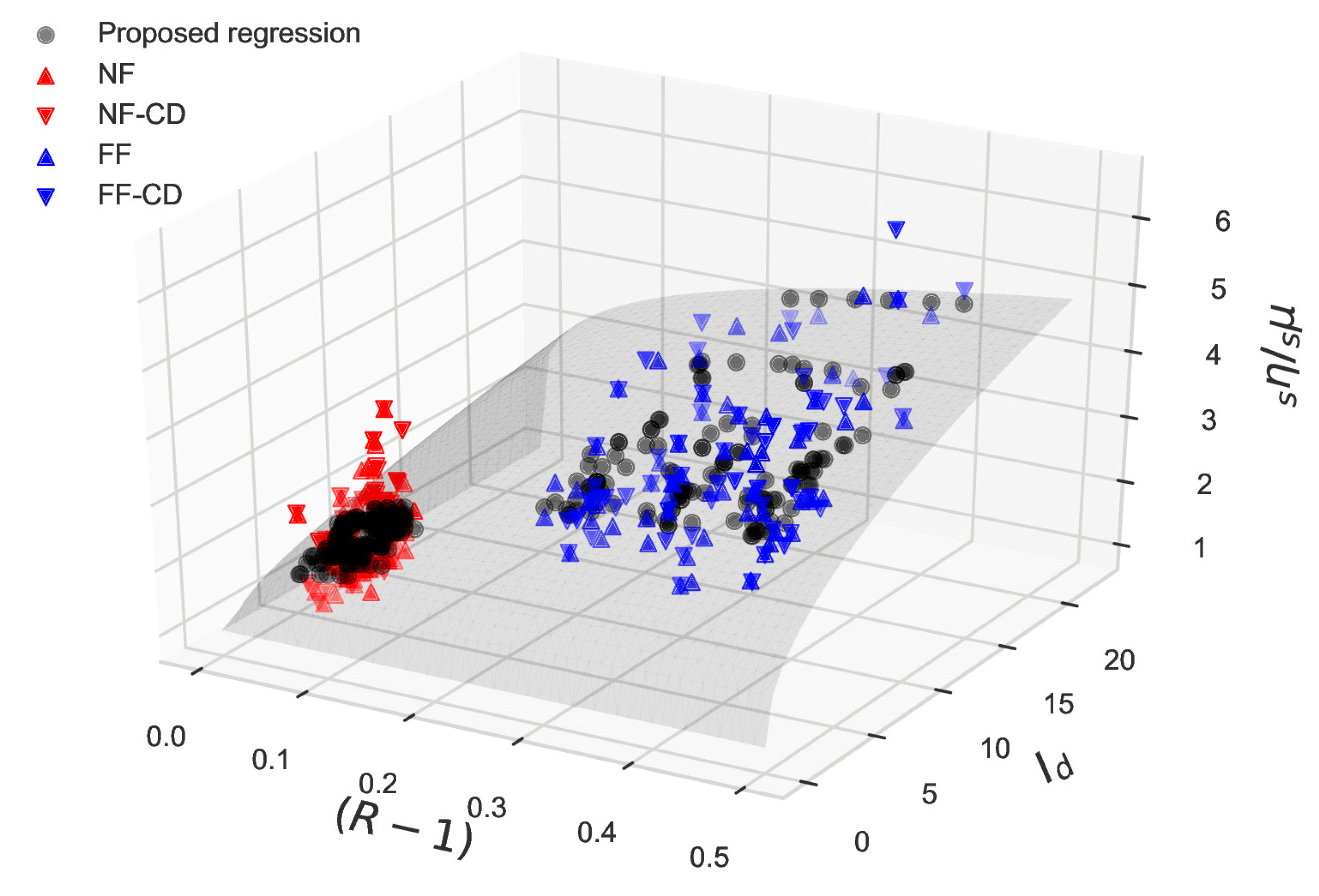
3.1. Estimation of Average _sη/_sμ of Dampers under Design Earthquake Hazard Level

The results at the end of the design earthquake hazard level showed that the inelastic demand concentrated at the dampers while the structure remained elastic, in both the with and without capacity design cases. Therefore, just the plastic response of the dampers is of interest herein. For each nonlinear time history analysis, the following variables were collected in a dataset: the ratio τ of the fundamental period T₁ to the initial period of medium T_g, the reduction factor R, the seismological parameter I_d, and the average cyclic demand parameter _sη/_sμ along the height of the building. Regular statistical procedures were used to analyse the results and find significant relationships between the variables. A preliminary principal component analysis was performed to determine the minimum number of variables that account for the most variation in the data, and found that the first two components (I_d and R) cover 92% of the variability of the data. On the other hand, a poor correlation between the parameter τ and the average value of _sη/_sμ was found. Figure 4 shows a scatter of these principal variables (R-1) and I_d versus the average cyclic demand parameter _sη/_sμ for each analysis in the dataset. Data is arranged around two clusters: near-fault seismicity in red, and far-field seismicity in blue.

It can be observed that far-field seismicity produces significantly higher values of _sη/_sμ. In Figure 4, the results from building models incorporating (or not) capacity design rules are plotted with triangles pointing downward or upwards respectively, and show very little variation one to each other. Using a non-linear least squares fitting, the average cyclic demand parameters of the dampers in a structure can be predicted with Equation (10) as a function of the principal variables, the strength reduction factor R and the seismological parameter I_d. The prediction with this equation is depicted in Figure 4 by the grey surface and black dots. Equation (10) correlates moderately with a regression score R² = 0.59.

$${}_s\mathsf{\eta }{/}_s\mathsf{\mu }=1+1.18·{\left(R-1\right)}^{0.24}·I_d^{0.44}$$

(10)

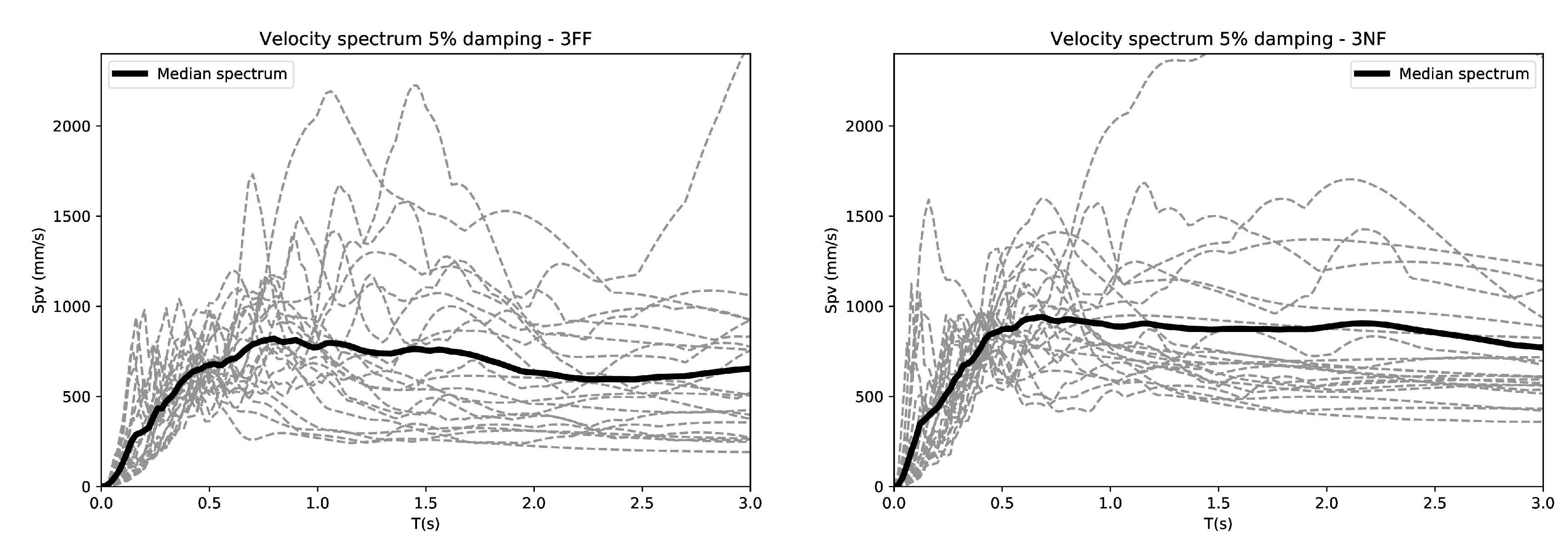
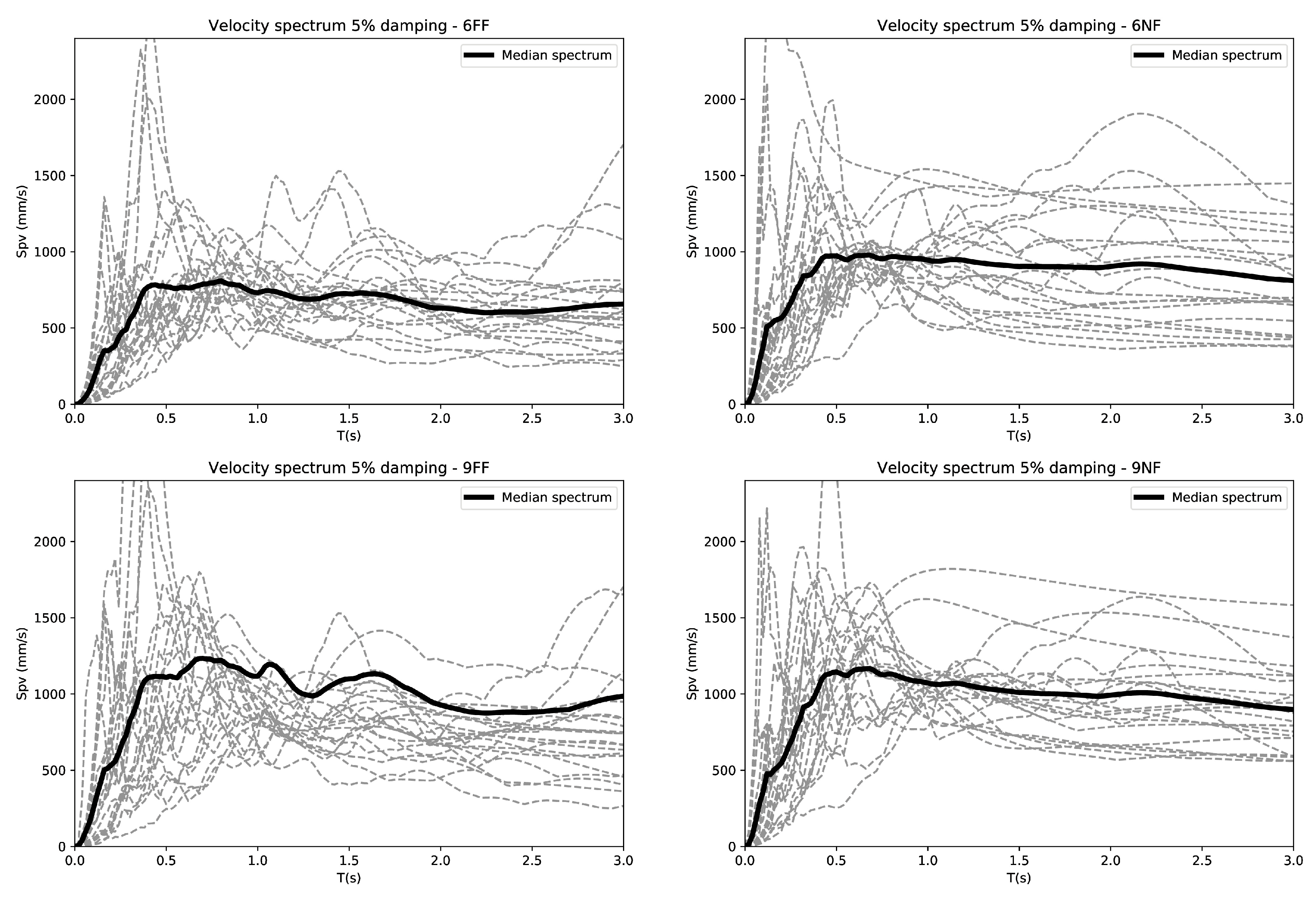
3.2. Behaviour of _sη/_sμ of Dampers and _fη/_fμ of Frames under the Maximum Considered Earthquake

In this study, the maximum considered earthquake that the structures were able to withstand was defined as that in which one of the dampers in the building reaches its ultimate energy dissipation capacity. The ultimate energy dissipation capacity was assessed using the damage model proposed by [30] and calibrated with the experimental results from a previous study [28]. At this earthquake level, plastic excursions are likely to occur on the reinforced concrete frame as well. For each nonlinear time history analysis under the maximum earthquake, the following variables were collected in a dataset: the parameter I_d of the ground motion, the number of equivalent inelastic cycles in the dampers _sη/_sμ, and the average _fη/_fμ in the reinforced concrete frame. Figure 5 shows the number of equivalent inelastic cycles for dampers and reinforced concrete frames against the seismological parameter I_d. Results for the hysteric dampers are shown with triangular markers with error bars (±1 standard deviation). In the case of frame elements, the average results are shown with triangular markers without error bars. The markers are pointing downwards for models that incorporate capacity design.

Under the maximum considered earthquake, the ratio _sη/_sμ in the dampers showed a tendency to increase with the parameter I_d, yielding lower values for near-fault records, and significantly larger values for far-field records. The maximum average values obtained for far-field records are about twice as much as the maximum values in the near-fault (14 vs. 7). The minimum average values are also double in the far-field (4 vs. 2). The average number of equivalent inelastic cycles in the reinforced concrete frame _fη/_fμ remains constant in the range 1–2, suggesting that there is no correlation with the seismological parameter I_d. Regarding the lateral collapse pattern of the frames, models of the weak-beam strong-column type are shown with triangular markers that point down, while frames with other collapse patterns are shown with markers that point up. Given the scatter of the results, it seems that the values of both ratios, _sη/_sμ and _fη/_fμ are not influenced by capacity design rules being enforced or not.

4. Discussion

The number of equivalent inelastic cycles N can be formulated as the ratio η/μ between the normalised dissipated energy η and the displacement ductility μ. This ratio is crucial to the design of hysteric dampers within the framework of performance-based design, as it quantifies the capacity to dissipate seismic energy for a given displacement. The ratio η/μ is also referred to as the efficacy of the dampers. The literature shows that the number of equivalent inelastic cycles varies for each specific lateral carrying system, and that it is strongly influenced by seismological parameters, especially by the intensity and the impulsive effects of the ground motion [16,17,25]. This study focused on mixed flexible-stiff structures, made of reinforced concrete frames with supplemental hysteric dampers under two levels of seismic hazard: the design earthquake and the maximum considered earthquake.

One interesting result is that the capacity design provisions in the gravity load resisting system, i.e., reinforced concrete frames has a negligible effect on the number of equivalent inelastic cycles of the dampers for both hazard levels. Because the efficacy of the dampers is independent of the lateral collapse pattern, the frame design can be neglected when designing the dampers. This is important in the retrofitting of pre-code frames that have undefined lateral collapse mechanisms. In light of these results, retrofitting strategies that focus on increasing the lateral deformability of the frames or preventing brittle failures (such as FRP wrapping) will have a greater impact on the performance of the dampers compared to strategies that focus on strengthening or reallocating plastic hinges.

Under the design earthquake, the ratio _sη/_sμ can be predicted as a function of the structural parameter R (the seismic force reduction factor, which relates the intensity of the ground motion and the lateral capacity of the structure), and the seismological parameter I_d, which has been shown to be an indicator of the impulsive effects of the ground motion. The tendency in the results is for larger ratios of _sη/_sμ as the parameters R and I_d increase. This latter parameter I_d accounts for most of the variability in the results, therefore it must drive the design of hysteretic dampers. Other parameters such as the ratio τ between the fundamental period and ground motion corner period show a poor correlation with _sη/_sμ in this type of structure and were neglected in the regression.

The maximum considered earthquake takes the structure to the onset of strength degradation in one of the dampers along the building, and allows for some structural damage to the reinforced concrete frames. Because some dampers reach their ultimate dissipation capacity in this scenario, the results of the ratio _sη/_sμ in the dampers should be taken as an upper-bound limit in the damper design. Our study confirmed that the efficacy of the dampers is significantly larger and more stable in the far-field. However, the ratio _fη/_fμ in the frame remains in the range of 1~2 for all analyses, which agrees with Akiyama’s [19] approximate design value of η/μ = 2 for bare elastic-plastic frames. Interestingly, the ratio _fη/_fμ is unchanged despite the impulsive effects of the ground motions, as it shows non-correlation to I_d. Because the efficacy of the frames is similar for far-field and near-fault seismicity, the matter of impulsivity can be neglected in the overall design and assessment of frames equipped with dampers.

References

1. Pnevmatikos, N.G.; Thomos, G.C. Stochastic structural control under earthquake excitations. Struct. Control Health Monit. 2014, 21, 620–633. [Google Scholar] [CrossRef]
2. Nikos, G. New strategy for controlling structures collapse against earthquakes. Nat. Sci. 2012, 4, 667–676. [Google Scholar] [CrossRef] [Green Version]
3. Symans, M.D.; Charney, F.A.; Whittaker, A.S.; Constantinou, M.C.; Kircher, C.A.; Johnson, M.W.; McNamara, R.J. Energy dissipation systems for seismic applications: Current practice and recent developments. J. Struct. Eng. 2008, 134, 3–21. [Google Scholar] [CrossRef] [Green Version]
4. Malhotra, P.K. Response of buildings to near-field pulse-like ground motions. Earthq. Eng. Struct. Dyn. 1999, 28, 1309–1326. [Google Scholar] [CrossRef]
5. Jangid, R.S.; Kelly, J.M. Base isolation for near-fault motions. Earthq. Eng. Struct. Dyn. 2001, 30, 691–707. [Google Scholar] [CrossRef]
6. Jangid, R.S. Optimum lead–rubber isolation bearings for near-fault motions. Eng. Struct. 2007, 29, 2503–2513. [Google Scholar] [CrossRef]
7. Providakis, C.P. Effect of LRB isolators and supplemental viscous dampers on seismic isolated buildings under near-fault excitations. Eng. Struct. 2008, 30, 1187–1198. [Google Scholar] [CrossRef]
8. Mazza, F.; Vulcano, A. Effects of near-fault ground motions on the nonlinear dynamic response of base-isolated rc framed buildings. Earthq. Eng. Struct. Dyn. 2012, 41, 211–232. [Google Scholar] [CrossRef]
9. Mollaioli, F.; Lucchini, A.; Cheng, Y.; Monti, G. Intensity measures for the seismic response prediction of base-isolated buildings. Bull. Earthq. Eng. 2013, 11, 1841–1866. [Google Scholar] [CrossRef]
10. Bhandari, M.; Bharti, S.D.; Shrimali, M.K.; Datta, T.K. The numerical study of base-isolated buildings under near-field and far-field earthquakes. J. Earthq. Eng. 2018, 22, 989–1007. [Google Scholar] [CrossRef]
11. Tirca, L.D.; Foti, D.; Diaferio, M. Response of middle-rise steel frames with and without passive dampers to near-field ground motions. Eng. Struct. 2003, 25, 169–179. [Google Scholar] [CrossRef]
12. Foti, D. Response of frames seismically protected with passive systems in near-field areas. Int. J. Struct. Eng. 2014, 5, 326–345. [Google Scholar] [CrossRef]
13. Dicleli, M.; Mehta, A. Effect of near-fault ground motion and damper characteristics on the seismic performance of chevron braced steel frames. Earthq. Eng. Struct. Dyn. 2007, 36, 927–948. [Google Scholar] [CrossRef] [Green Version]
14. Filiatrault, A.; Tremblay, R.; Wanitkorkul, A. Performance evaluation of passive damping systems for the seismic retrofit of steel moment-resisting frames subjected to near-field ground motions. Earthq. Spectra 2001, 17, 427–456. [Google Scholar] [CrossRef]
15. Xu, Z.; Agrawal, A.K.; He, W.L.; Tan, P. Performance of passive energy dissipation systems during near-field ground motion type pulses. Eng. Struct. 2007, 29, 224–236. [Google Scholar] [CrossRef]
16. Donaire-Ávila, J.; Mollaioli, F.; Lucchini, A.; Benavent-Climent, A. Intensity measures for the seismic response prediction of mid-rise buildings with hysteretic dampers. Eng. Struct. 2015, 102, 278–295. [Google Scholar] [CrossRef]
17. Benavent-Climent, A. An energy-based method for seismic retrofit of existing frames using hysteretic dampers. Soil Dyn. Earthq. Eng. 2011, 31, 1385–1396. [Google Scholar] [CrossRef]
18. Zahrah, T.F.; Hall, W.J. Earthquake energy absorption in SDOF structures. J. Struct. Eng. 1984, 110, 1757–1772. [Google Scholar] [CrossRef]
19. Akiyama, H. Earthquake-Resistant Limit-State Design for Buildings; University of Tokyo Press: Tokyo, Japan, 1985. [Google Scholar]
20. Akiyama, H. Earthquake resistant design based on the energy concept. In Proceedings of the 9th WCEE, Tokyo-Kyoto, Japan, 2–9 August 1988; pp. 905–910. [Google Scholar]
21. Akiyama, H. Collapse modes of structures under strong motions of earthquake. Ann. Geophys. 2002, 45, 791–798. [Google Scholar]
22. Malhotra, P.K. Cyclic-demand spectrum. Earthq. Engng. Struct. Dyn. 2002, 31, 1441–1457. [Google Scholar] [CrossRef]
23. Kunnath, S.K.; Chai, Y.H. Cumulative damage-based inelastic cyclic demand spectrum. Earthq. Eng. Struct. Dyn. 2004, 33, 499–520. [Google Scholar] [CrossRef]
24. Manfredi, G. Evaluation of seismic energy demand. Earthq. Eng. Struct. Dyn. 2001, 30, 485–499. [Google Scholar] [CrossRef]
25. Manfredi, G.; Polese, M.; Cosenza, E. Cumulative demand of the earthquake ground motions in the near source. Earthq. Engng. Struct. Dyn. 2003, 32, 1853–1865. [Google Scholar] [CrossRef]
26. Park, Y.J.; Reinhorn, A.M.; Kunnath, S.K. Inelastic Damage Analysis of Reinforced Concrete Frame–Shear-Wall Structures (IDARC); Technical Report NCEER-87-0008; National Center for Earthquake Engineering Research: Buffalo, NY, USA, 1987. [Google Scholar]
27. Kunnath, S.K.; Reinhorn, A.M.; Abel, J.F. A computational tool for evaluation of seismic performance of reinforced concrete buildings. Comput. Struct. 1991, 41, 157–173. [Google Scholar] [CrossRef]
28. Benavent-Climent, A.; Morillas, L.; Vico, J.M. A study on using wide-flange section web under out-of-plane flexure for passive energy dissipation. Earthq. Eng. Struct. Dyn. 2011, 40, 473–490. [Google Scholar] [CrossRef]
29. Ambraseys, N.; Smit, P.; Douglas, J.; Margaris, B.; Sigbjörnsson, R.; Olafsson, S.; Suhadolc, P.; Costa, G. Internet site for European strong-motion data. Boll. Geofis. Teor. Appl. 2004, 45, 113–129. [Google Scholar]
30. Benavent-Climent, A. An energy-based damage model for seismic response of steel structures. Earthq. Eng. Struct. Dyn. 2007, 36, 1049–1064. [Google Scholar] [CrossRef]
Figure 1. Energy dissipation in an elastoplastic system: (a) Cyclic force-displacement Q-δ curve; (b) Energy dissipated by yielding EH; (c) Energy dissipated in a quarter-cycle at maximum displacement.
Applsci 10 04364 g001
Figure 2. Load-deformation curves in flexible-stiff mixed systems: (a) flexible part; (b) stiff part; (c) mixed system.
Applsci 10 04364 g002
Figure 3. Schematic of the structural model.
Applsci 10 04364 g003
Figure 4. Proposed regression of principal features and sη/sμ.
Applsci 10 04364 g004
Figure 5. Values of sη/sμ of dampers and fη/fμ of frames under the maximum considered earthquake.
Applsci 10 04364 g005