Abstract
Recurrent neural networks (RNNs) can model the time-dependency of time-series data. It has also been widely used in text-dependent speaker verification to extract speaker-and-phrase-discriminant embeddings. As with other neural networks, RNNs are trained in mini-batch units. In order to feed input sequences into an RNN in mini-batch units, all the sequences in each mini-batch must have the same length. However, the sequences have variable lengths and we have no knowledge of these lengths in advance. Truncation/padding are most commonly used to make all sequences the same length. However, the truncation/padding causes information distortion because some information is lost and/or unnecessary information is added, which can degrade the performance of text-dependent speaker verification. In this paper, we propose a method to handle variable length sequences for RNNs without adding information distortion by truncating the output sequence so that it has the same length as corresponding original input sequence. The experimental results for the text-dependent speaker verification task in part 2 of RSR 2015 show that our method reduces the relative equal error rate by approximately 1.3% to 27.1%, depending on the task, compared to the baselines but with an associated, small overhead in execution time.
1. Introduction
Recurrent neural networks (RNNs) are neural networks used to model time-series data. In addition to the original connections (i.e., from input to hidden states), it has recurrent connections from the hidden states of the previous time step to those of the current time step. Both connections are shared over all time steps. In each time step, the RNN memorizes the hidden states in the current time step (computed from both the input at the current time step and the hidden states at the previous time step). It feeds this information to the next time step. This means that the hidden states in the current time step recursively include information from all the previous states. Therefore, RNNs can effectively model the global context information of an input sequence with a small number of parameters.
Due to this advantage, RNNs have been successfully adapted for speaker verification, especially for text-dependent speaker verification (TD-SV) [1,2,3,4,5]. TD-SV is a technique to verify both a user’s identity and a phrase using the utterance. In TD-SV, the available lexicon is constrained for a few types of phrases, and both enrollment and test utterances should have the same phrase. In real applications, TD-SV is mainly used in various smart devices that require user verification to unlock the devices. In most cases, the phrases of utterances are constrained to few keywords for both user convenience and low verification error, such as “Ok Google” for Google Assistant [6] and “Hi Bixby” for Samsung Bixby [7]. The short keyword-based utterances are particularly vulnerable to information distortion, because short keywords are considered completely different even if they are only slightly changed. For example, the utterance of “Hi Bixby” and that of “Hi Bixb” are considered different classes of utterance in TD-SV, even if these utterances are from the same speaker. Therefore, it is important to model short utterances with minimization of information distortion. RNNs can effectively model not only speaker information but also phrase information in utterance. In TD-SV, the RNN in a speaker-and-phrase-discriminant network is used for mapping variable-length utterance to a fixed-size vector (this fixed-size vector is usually called embedding). The embedding is expected to represent both speaker and phrase information in the utterance. It can be either the output frame from the last time step or part of temporal pooling (e.g., running average along time axis) of the output sequence. In this paper, we focus on the latter method, temporal pooling, because it has been empirically confirmed that temporal pooling has higher performance [2].
Like other kinds of neural networks, RNNs are also trained in mini-batch units. To feed a set of input sequences into an RNN in mini-batch units, all the sequences in a given mini-batch must be the same length (denoted as the target length). In most cases, however, input sequences have variable lengths, furthermore, we do not know the length of the sequences in advance. In general, truncation/padding is used to make sure all variable-length sequences have the same target length. Based on the target length, the longer sequences are truncated, and the shorter sequences are padded. Note that there is no specific criterion for setting the target length, and the target lengths are different on a case by case basis. However, truncation/padding cannot avoid information distortion of the original sequences (i.e., sequences that have not been truncated/padded), because truncation brings a loss of some existing information, and padding brings additional unnecessary information not in the original. This problem may degrade the performance of TD-SV, especially when utterances are very short (i.e., short keyword-based TD-SV). Because the short utterance is vulnerable to information distortion, as mentioned above. Sequential processing is an alternative way to avoid this information distortion: feed only one input sequence at a time (i.e., the size of mini-batch is 1), repeat the feeding for all given sequences, and then gather the outputs over the mini-batch. Nonetheless, we do not consider sequential processing in this paper, it is too inefficient in terms of computation speed. Multi-processing can be used in order to speed up the sequential processing but this becomes too inefficient in terms of memory usage.
There are some advanced implementations being used in popular deep learning platforms to reduce information distortion caused by truncation/padding. TensorFlow [8] supports the cudnn_rnnv3 method (In tensorflow.python.ops.gen_cudnn_rnn_ops. However, it is not officially supported and cannot be found in the official documents.) method, which is a kind of RNN implementation backed by cuDNN [9]. Similarly, PyTorch [10] supports the PackedSequence class and related methods. Even if all the input sequences in a mini-batch are padded to have the target length (The padding is optional in PyTorch.) so they have some padded frames, these implementations compute the output sequences with the original frames only. In this paper, the frame corresponds to an element of the sequence. The computation can be executed in parallel (i.e., in mini-batch units). Therefore, each output sequence has the same length as the corresponding original input sequence. All the output sequences are then padded with zero to ensure these have the target length. For example, consider a sample input sequence of length in a mini-batch, and the target length is (). Regardless of padding, the output sequence for is computed up to the time , that is, . Then, is padded with zero, that is, where is a zero-vector. However, there are still unnecessary values in the output sequences. Therefore, these implementations also cannot be free from information distortion.
In this paper, we propose a method to remove the information distortion. After the output sequences are computed from the padded input sequence, the proposed method simply truncates the output sequence to have the same length as the original input sequence. Therefore, the proposed method can produce the same output sequence as the output sequence that would result from the original input sequence. We expect that the proposed method gives performance improvement on TD-SV tasks with some computing overhead.
2. Conventional Methods to Handle Variable Length Sequences
Truncation/padding is a conventional and popular method to make sure all input sequences in a mini-batch have the same target length. There are three things that should be considered before truncation/padding. First, how long all the input sequences will be (i.e., target length). Second, where truncation/padding will be applied (i.e., position). Third, if padding is required, what values will be padded (i.e., padding value). In addition, we can also consider the use of advanced implementations, such as cudnn_rnnv3 or PackedSequence.
2.1. Target Length
All the input sequences in a mini-batch are truncated/padded to have the same target length. There are four types of target length: global maximum, global mean, batch maximum, and batch mean. For example, consider the 9 input sequences with the lengths (see Figure 1). The size of a mini-batch is 3: , , and are in the first mini-batch, , , and are in the second mini-batch, and , , and are in the third mini-batch. Note that in the example it is assumed that truncation/padding is applied at the end of each sequence.
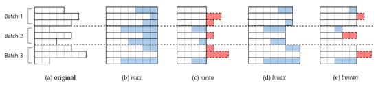
Figure 1.
Examples using four types of target length based on an (a) original: (b) max, (c) mean, (d) bmax, and (e) bmean. The white frames represent original input frames. The blue frames represent padded frames. The red frames represent truncated frames.
2.1.1. Global Maximum
Global maximum (denoted as max) means that the target length is the length of the longest sequence over given dataset. In our example (Figure 1b), all sequences are padded to have a length of 7, regardless of which mini-batch each sequence belongs to. The length of 7 corresponds to the length of the longest sequence (i.e., the length of ). This leads to a total padded length of 24 in this example.
There is no information loss because no sequence is truncated. Also, all the sequences can be padded in advance because the target length is fixed over the entire process. However, this method generally leads to the greatest addition of unnecessary information and the corresponding extra computation.
2.1.2. Global Mean
Global mean (denoted as mean) means that the target length is set to the average length of all the sequences over the given dataset. In the example (Figure 1c), the average length is 4 (the decimal point is rounded off). The sequences shorter than 4 (i.e., , , and ) are padded, and those longer than 4 (i.e., , , , , and ) are truncated to have a length of 4. The total truncated and padded lengths are 8 and 5, respectively, and therefore, the total amount of computation is decreased compared to global maximum.
It has a relatively smaller computation burden. Also, like in max, all the sequences can be padded in advance. However, it is almost inevitable there is information distortion because there are both truncated and padded sequences.
2.1.3. Batch Maximum
Batch maximum (denoted as bmax) means that the target length is the length of the longest sequence in the current mini-batch. In the example (Figure 1d), the sequences in batch 1, 2, and 3 are padded to have lengths of 6, 5, and 7, respectively. The lengths of 6, 5, and 7 correspond to the length of the longest sequence over the sequences in batch1, 2, and 3 (i.e., the lengths of , , and ), respectively. The total padded length is 15 in the example.
There is no information loss, as in max. The amounts of additional unnecessary information and the corresponding computation burden are relatively less than in max. However, we cannot pad the sequences in advance, so we incur an additional overhead for padding. In many cases, the order of training data is changed with each epoch, and therefore, the target length is also changed with each iteration.
2.1.4. Batch Mean
Bach mean (denoted as bmean) means that the target length is the average length of sequences in the current mini-batch. In the example (Figure 1e), the sequences in batch1, 2, and 3 are padded to have lengths of 5, 3, and 5, respectively. The lengths of 5, 3, and 5 correspond to the length of the average length of the sequences in batch1, 2, and 3 (the decimal point is rounded off), respectively. The total truncated and padded lengths are both 5, and therefore cancel each other out so the total computation amount is not changed.
This method may incur the smallest computation burden, especially when the standard deviation of the sequence lengths is large. However, it is inevitable there is significant information distortion, as in mean. It also requires overhead in truncation/padding for the same reason as in bmax because we cannot pad the sequences in advance.
2.2. Position
First, note that we do not consider bidirectional RNNs, and the RNNs mentioned in this paper are all unidirectional. In an RNN, the state at the current time step is affected by all states over the previous time steps. In contrast, the state at the current time step does not affect all the previous states, and affects only the states in all the following time steps. Naturally, the outputs are affected by the truncation/padding position. Figure 2 shows an example for position. In the example, the target length is 4, and the black arrow indicates the first time step of the original sequence.
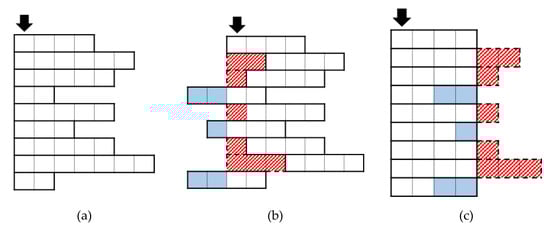
Figure 2.
The example of two types of truncation/padding position based on an (a) original: (b) front and (c) end. The black arrow indicates the first time step of the original sequence.
2.2.1. Front
In this case, truncation/padding is applied at the front of the sequence (Figure 2b).
The truncated sequence loses information contained in the front sections of the original sequence. This can cause performance degradation in task where the information at the front is more important than that at the end. For example, consider the discrimination of two utterances with the phrases: “light off” and “oven off”. If some of the front frames are truncated and only the frames corresponding to “off” remain, we cannot discriminate the meaning between these utterances.
In a padded sequence, the padded frames affect the original frames. In other words, the last hidden state from the padded frames becomes the initial states of the original frames. The last hidden state from the padded frames is generally not zero, even if all the padded values are zero, due to the biases and activation function. Therefore, the original frames are affected by the padded frames.
2.2.2. End
In this case, truncation/padding is applied at the end of the sequence (Figure 2c).
The truncated sequences lose the information contained in the end sections of the original sequence. This can cause performance degradation on a task in which the information at the end is more important than that at the front. For example, consider the discrimination of two utterances with the phrases: “volume up” and “volume down”. If some of the end frames are truncated and only the frames corresponding to “volume” remain, we cannot discriminate the meaning between these utterances.
In padded sequences, the original frames affect the padded frames. Unlike in front, the original frames are not affected by the padded frames. Therefore, the values of the outputs from the original frames are not changed. It means that we can obtain exactly the same outputs as the original sequence would give, if we can remove only the outputs from the padded frames.
2.3. Padding Value
2.3.1. Constant
All the padded values are the same regardless of sequence (denoted as const). In most cases, zero is used as the padding value, and we also apply zero-padding in this paper. Padding with a constant value means that all sequences are given common information because all sequences are given the same values. Therefore, this may degrade the ability to discriminate between sequences.
2.3.2. Repeat
A sequence is padded by repeating some of its own frames (denoted as rept). For example, consider a sample input sequence of length 4, and we want to make the length of = 6 by padding. The padded sequence becomes for front and for end. As each utterance is padded with some frames from itself, it can maintain its own unique speaker information. However, at the same time the identity of the phrase is changed, this may degrade the ability to discriminate between phrases.
2.4. Advanced Implementation
In this paper, we focus on PackedSequence and its methods in PyTorch. Note that our purpose is not a comparison between the deep learning platforms, and the outputs from TensorFlow and PyTorch are the same.
Figure 3 shows the procedure for PackedSequence, which proceed in four steps. We start with a list of sequences that have variable lengths (e.g., , , and that have the length of 3, 5, and 4, respectively). Note that each sequence is a tensor object, but a list of the sequences is a simple Python list object. First, the sequences are sorted by length in descending order (The sorting is not required, but recommended.) (e.g., the order , , ). Second, the sorted sequences are converted into a PackedSequence object, which is done by the pack_sequence method. The PackedSequence object merges all separate sequences into one sequence with the batch_sizes attribute. In the PackedSequence object, all frames in the mini-batch are arranged in time step order. In the example, the list of the sequences is converted into a single sequence: . The batch_sizes attribute gives the number of frames at each time step to feed into the RNN. In the example, the batch_sizes becomes . Third, the PackedSequence object is fed into the RNN. The output is also a PackedSequence object. Fourth, the output object is converted to a list of tensor objects where all the output sequences have the same length. The PackedSequence object should be converted to a general tensor object, because it can be used only for RNN objects. Zero-padding is applied, and the target length is the length of the longest sequence in the mini-batch (e.g., 5; the length of ). This can be done by pad_packed_sequence method. Therefore, we can obtain the same outputs as from sequential processing, except for the zero-padded frames in the outputs.
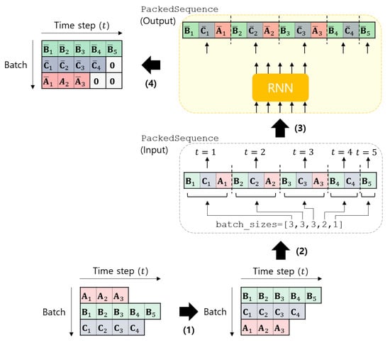
Figure 3.
The procedure of the PackedSequence object in PyTorch.
3. The Proposed Method
In this paper, we proposed a simple method to handle variable length sequences for RNNs without information distortion. All the input sequences must be pre-processed with a target length of max/bmax and the position of end (i.e., max_end_* or bmax_end_*), or with PackedSequence. With these conditions, there is no information loss, and the original frames are not affected by the padded frames.
The bottom of Figure 4 and Algorithm 1 show the overview and pseudo code of the proposed method, respectively. Consider the set of output sequences in a mini-batch of size . All the output sequences in has the same length , which are computed from the padded input sequences. For each mini-batch, each output sequence ) is first truncated to have its original length . The truncation is applied at the end of the sequence, that is, the truncated sequence is ). Each truncated sequence is then used to compute the embedding by temporal pooling. With the baseline methods, the embedding is computed using rather than . With the proposed method, therefore, we can exclude the effects of the padded frames in the output sequence from the embedding.
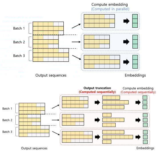
Figure 4.
The overview of the (top) conventional and (bottom) proposed methods. The yellow frames represent the output from the original input frame. The gray frames represent the output from the padded frame. The green elements represent an embedding.
Regardless of the kinds of pre-processing method (i.e., the baseline and the proposed), we used two kinds of temporal pooling (i.e., in Algorithm 1) for computing embeddings. One is simply running average of the output sequence along time axis. In this case, the embedding becomes either (for the baseline) or (for the proposed). The other is running weighted sum of the output sequence along time axis. In this case, the embedding becomes either (for the baseline) or (for the proposed), where is the attention weight for the -th output frame obtained by a self-attention mechanism [11,12].
| Algorithm 1 The pseudo code of the proposed method |
| Input |
| : list of the output sequences. Each sequence has the shape of |
| : list of the original lengths of each sequence ( for all i). |
| n: mini-batch size. |
| T: target length. |
| D: the dimensionality. |
| Output |
| : list of the embeddings. All the embeddings are D-dimensional. |
| 1: # empty list |
| 2: for i in range(n): # for the i-th output sequence |
| 3: # output truncation up to its original sequence |
| 4: # the i-th embedding |
| 5: # append the i-th embedding into the list |
| 6: return # convert to tensor object |
In the proposed method, computing embeddings from output sequences cannot be performed in mini-batch units (i.e., cannot be computed in parallel), because all the original sequences generally have variable lengths. Also, there is an additional overhead for the output truncation. Therefore, the proposed method is slower than the baseline method. Nonetheless, we expect that the execution time between the baseline and proposed method do not differ significantly. This is due to the fact that most of the time is occupied by the RNN operation itself, which can be processed in mini-batch units (i.e., can be computed in parallel) for both the baseline and proposed method.
4. Experiment
4.1. Database
We used part 2 of the robust speaker recognition (RSR) 2015 dataset [13], which is designed for TD-SV. Part 2 focuses on device control and speaker verification simultaneously using fixed command words. It consists of utterances from 300 speakers, and is divided into background, development, and evaluation subsets. The background and development sets are comprised of 50 male and 47 female speakers. The evaluation set is comprised of 57 male and 49 female speakers. There is no speaker overlap across the three subsets. Each speaker speaks 30 kinds of utterance in 9 different sessions. The length of utterance, including silence, is 1.99 s on average and they range from 1.66 to 2.44 s. Excluding silence part, the length of utterances is 0.63 s on average and they range from 0.44 to 0.99 s.
The background set is used to build gender-independent models. The development set is used to validate the performance with gender independent trials. The evaluation set is used to evaluate the performance of the trained models with gender dependent trials. A target trial means the case where both speaker and phrase are the same between the enroll and test utterances. A non-target trial means the case where either the speaker or phrase is different between the enroll and test utterances. Note that the enrollment model in trials of RSR 2015 consists of 3 utterances. We used an average of 3 embeddings along the time axis as the enrollment model. We validated the performance of the models for every epoch. The models that showed the best performance in the development trials were used for evaluation.
4.2. Experimental Setup
We used 40-dimensional log mel filterbank coefficients as the acoustic feature for each frame. For each utterance, 25 ms frames were extracted at 10 ms intervals. We applied pre-processing for each frame in the following order: removing DC offset, pre-emphasis filtering with a coefficient of 0.97, and Hamming windowing. The number of FFT points was 512. After the feature extraction, mean normalization was applied with a 300-frame sliding window. Silence frames were removed by energy-based voice activity detection (VAD). For each utterance, the sequence of log energies passed the median filter with a kernel size of 11, and then was normalized to have zero mean and a unit variance. The energies were modeled using a tied-variance Gaussian mixture model (GMM) with 3 components. Each of the components represented high, middle, and low energies. The frames that correspond to the component with low energy are removed. After the VAD, the number of frames is 86 on average, has the standard deviation of about 30.7, and range from 15 to 501, which means that our VAD cannot perfectly remove silence frames only. Nevertheless, we empirically found that our VAD is more efficient than the general VAD. The Kaldi toolkit [14] was used to extract mel filterbank. The scikit-learn [15] was used to implement the GMM for VAD.
We built a speaker-and-phrase-discriminant network based on a two-layer long short-term memory (LSTM) [16]. Each layer of the LSTM has 512 units. The 512-dimensional embedding was extracted by averaging the output sequences along the time axis, or by a self-attention mechanism. The number of attention heads of the self-attention is 4. Batch normalization [17] was applied to the embedding. Two softmax classifiers (i.e., one for classifying speakers, and one for classifying phrases) are stacked on the top of the LSTM. All the weights of the LSTM were initialized using the Glorot normal distribution [18]. The recurrent weights were orthogonalized [19]. The forget biases were initialized to one [20], and the other biases of the LSTM were initialized to zero. The weights of both the attention layer and classifiers were orthogonalized. There is no bias in both the attention layer and classifiers. AMSGrad [21], a variant of the Adam [22] optimizer, was used to minimize the cross-entropy loss. The learning rate was fixed at . We trained the network for 100 epochs with a mini-batch size of 32, we then selected the best network by validation. PyTorch was used to implement the network.
We trained the networks with the 18 different methods (i.e., 16 kinds of truncation/padding, the PackedSequence based implementation, and the proposed method). In contrast, we validate and evaluate only with the proposed method. For a fair comparison, it is natural that all the systems should be evaluated under the same condition, regardless of the kinds of pre-processing method for input sequence used in the training phase. Also, in real applications, it is assumed that only one sequence is fed into the network at one time. Hence, there is no need to apply truncation/padding. However, it takes a long time to feed only one sequence into the network at one time. Therefore, we used the proposed method instead for both validation and evaluation, which can bring the same results as when feeding one sequence into the network at one time with less computation time. Cosine similarity was used as the scoring metric, and equal error rate (EER) was used as the evaluation metric. All our experiments were conducted using NVIDIA Quadro RTX 8000 GPU and Intel Xeon E5-2699 v4 CPU.
4.3. Results
Table 1 shows the EERs on the trials of both development and evaluation sets according to the methods for handling variable length sequences without self-attention. On average, max/bmax showed relatively lower EERs of about 9.2% than mean/bmean. This means that the loss of information from truncation is worse than the addition of unnecessary information from padding.

Table 1.
The EERs (%) of systems without self-attention on the development and evaluation trials of RSR 2015 part 2. The lowest EERs among all the methods are highlighted in bold, the lowest EERs among all the methods except the proposed method are underlined.
On the other hand, against our expectation, there was no consistent trend with the other conditions. For example, const did not always show higher EERs than rept. Also, front did not always show lower EERs than end, unlike in [23]. Notice that both speaker information and phrase information are important in TD-SV. In general, const can maintain the identity of phrase, although the discriminative power between speakers can be degraded. Whereas, rept can maintain speaker information, although the identity of phrase is somewhat changed. It can be seen that there is a trade-off between const and rept, while there is no significant difference between front and end in TD-SV.
Except on the female evaluation trials, the proposed method showed the lowest EERs, exhibiting relative reductions of approximately from 1.3% (i.e., compared with PackedSequence) to 27.1% (i.e., compared with bmean_front_rept) in the development trials, and from 3.8% (i.e., compared with PackedSequence) to 20.8% (i.e., compared with mean_front_rept) on the male evaluation trials. These results correspond with our expectations that reducing the information distortion can improve performance, and it is shown that the proposed method can remove information distortion.
On the female evaluation trials, the max_end_rept showed the lowest EER. The proposed method showed the second lowest EER, but only relatively about 0.2% higher than the max_end_rept. Therefore, it is difficult to say that there is a significant difference between them.
Table 2 shows the EERs with self-attention. Attention emphasizes more important frames by applying different weights. As in Table 1, max/bmax still show relatively lower EERs of approximately 7.6% than mean/bmean in general. Even so, the gap between the EERs was slightly decreased, relatively about from 9.2% to 7.6%. This means that attention can compensate for information loss somewhat.
Table 2.
The EERs (%) of systems with self-attention on the development and evaluation trials of RSR 2015 part 2. The lowest EERs among all the methods are highlighted in bold, the lowest EERs among all the methods except the proposed method are underlined.
If attention can perfectly ignore (i.e., give zero attention weight) the frames that contain unnecessary information, the EERs of max/bmax/PackedSequence (i.e., when there is no information loss) may be very close to those of the proposed method. If so, it is not necessary to use the proposed method. In practice, however, the proposed method showed relatively about 11.2%, 11.1%, and 6% lower EERs on average than max, bmax, and PackedSequence, respectively. Except on the development trials, the proposed method shows the lowest EERs, exhibiting relative reductions of from approximately 7.7% (i.e., compared with bmax_front_rept) to 24.6% (i.e., compared with bmean_end_rept) on the male evaluation trials, and from 3.1% (i.e., compared with bmax_front_const) to 20.8% (i.e., compared with bmean_end_rept) on the female evaluation trials. This means that attention cannot perfectly remove the unnecessary information. When using the conventional methods, which cause information distortion, the attention weights can also be distorted because they were trained using the frames that have distorted information. Therefore, the proposed method is required to remove the information distortion.
On the development trials, the max_front_rept and max_end_rept showed the lowest and second lowest EERs, respectively. The proposed method showed the third lowest EER with relative about 1.8% and 0.3% higher than the max_front_rept and max_end_rept, respectively. It seems that the network trained with a sequence that includes some unnecessary information may be more suitable for the embedding from the sequence (that includes some unnecessary information) rather than the embedding from the distortion-free sequence.
Table 3 shows the average execution time for extracting one embedding with/without attention. In our experiments, execution time is proportion to both computation amount and memory usage because we did not use the multi-processing method. Naturally, max, which requires the most amount of computation, shows the longest execution times. Also, in most cases, the methods with attention show longer execution times, relatively about 7.4%.
Table 3.
Average execution time (ms) for extracting one embedding.
bmax showed relatively shorter execution times of approximately 88.8% than max, and bmean showed relatively shorter execution times of approximately 66.7% than mean. Notice that there is a trade-off between max/mean and bmax/bmean. Generally, max/mean require more computation than bmax/bmean. Instead, bmax/bmean require an overhead for truncation/padding because the target length is changed for every mini-batch. This overhead is not required with max/mean because the target length is fixed, and therefore, the truncation/padding is applied in advance. In the case that the standard deviation of the number of frames is somewhat large, like in our experiments (i.e., 30.7), reducing the amount of computation using bmax/bmean is more effective to reduce execution time than applying truncation/padding in advance using max/mean. On the contrary, in the case that the standard deviation is small enough, applying truncation/padding in advance can be more effective than reducing the amount of computation. Therefore, it is necessary to select proper method depending on the database used. On the other hand, there is no significant difference according to position or padding value.
In our experiments, the proposed method is applied to the output sequences obtained by PackedSequence. The proposed method shows longer execution times than PackedSequence (a relative increase about 33.7%). The increased execution time is due to the output truncation and sequential processing.
Recall that the female evaluation trial in Table 1 (i.e., without attention) and the development trial in Table 2 (i.e., with attention), where max showed lower EERs than the proposed method. The max reduced relatively lower EERs of approximately from 0.2 to 1.8%. However, the max revealed far longer execution times, increased approximately from 6.7 times to 8.4 times. In real applications, therefore, use of the max is not good choice when considering not only EER but also execution time, even though the max exhibited lower EERs than the proposed method on those trials.
5. Conclusions
In this paper, we proposed a simple, novel method to handle variable length sequences for RNNs without information distortion. The prerequisites of this proposed method are to apply padding at the end of sequences to make all the input sequences in a mini-batch the same length or use PackedSequence in PyTorch, so that any padded frames do not affect the original frames. The key point of the proposed method is the output truncation. For each output sequence in a mini-batch, we truncate the outputs to remove the padded frames so all that remains is the outputs from the original input frames. The proposed method mostly showed lower EERs on part 2 of the RSR 2015 task but with a small associated overhead in computation time. Even though there are some cases where the proposed method showed higher EERs, the proposed method showed far less execution times than the baselines. Based on these results, we believe that the proposed method generally gives more robust performance than the conventional methods, when considering both error rate and execution time.
In the future, we will evaluate our proposed method with RNNs in other tasks, such as speech recognition and natural language processing, to confirm the generalization power of the proposed method. Moreover, we will investigate the distortion-free method for other kinds of neural networks, such as convolutional neural networks (CNNs). The information distortion caused by truncation/padding can also be observed when using other kinds of neural networks. However, the proposed method can be used for RNNs only because the effects of truncation/padding depends on the kinds of neural networks. Therefore, it can be useful to develop the distortion-free methods for other kinds of neural networks.
Author Contributions
Conceptualization, S.-H.Y.; methodology, S.-H.Y.; investigation, S.-H.Y.; writing—original draft preparation, S.-H.Y.; writing—review and editing, H.-J.Y.; supervision, H.-J.Y. All authors have read and agreed to the published version of the manuscript.
Funding
This research was supported by Projects for Research and Development of Police Science and Technology under the Center for Research and Development of Police Science and Technology and the Korean National Police Agency funded by the Ministry of Science, ICT and Future Planning (PA-J000001-2017-101).
Conflicts of Interest
The authors declare no conflict of interest. The funders had no role in the design of the study; in the collection, analyses, or interpretation of data; in the writing of the manuscript, or in the decision to publish the results.
References
- Heigold, G.; Moreno, I.; Bengio, S.; Shazeer, N. End–to–end text–dependent speaker verification. In Proceedings of the IEEE International Conference on Acoustics, Speech, and Signal Processing (ICASSP), Shanghai, China, 20–25 March 2016; pp. 5116–5119. [Google Scholar]
- Bhattacharya, G.; Kenny, P.; Alam, J.; Stafylakis, T. Deep neural network based text–dependent speaker verification: Preliminary results. In Proceedings of the Odyssey, Pyatigorsk, Russia, 6–9 June 2016; pp. 9–15. [Google Scholar]
- Zhang, S.; Chen, Z.; Zhao, Y.; Li, J.; Gong, Y. End–to–end attention based text–dependent speaker verification. In Proceedings of the IEEE Spoken Language Technology Workshop (SLT), San Diego, CA, USA, 13–16 December 2016; pp. 171–178. [Google Scholar]
- Wan, L.; Wang, Q.; Papir, A.; Moreno, I.L. Generalized end–to–end loss for speaker verification. In Proceedings of the IEEE International Conference on Acoustics, Speech, and Signal Processing (ICASSP), Calgary, AB, Canada, 10–15 April 2018; pp. 4879–4883. [Google Scholar]
- Chowdhury, F.A.R.R.; Wang, Q.; Moreno, I.L.; Wan, L. Attention–based models for text–dependent speaker verification. In Proceedings of the IEEE International Conference on Acoustics, Speech, and Signal Processing (ICASSP), Calgary, AB, Canada, 15–10 April 2018; pp. 5359–5363. [Google Scholar]
- Access the Google Assistant with Your Voice. Available online: https://support.google.com/assistant/answer/7394306 (accessed on 5 March 2020).
- Talk to Bixby Using Voice Wake–Up. Available online: https://www.samsung.com/us/support/answer/ANS00080448 (accessed on 5 March 2020).
- Abadi, M.; Barham, P.; Chen, J.; Chen, Z.; Davis, A.; Dean, J.; Devin, M.; Ghemawat, S.; Irving, G.; Isard, M.; et al. TensorFlow: A system for large–scale machine learning. In Proceedings of the 12th USENIX Symposium on Operating System Design and Implementation (OSDI), Savannah, GA, USA, 2–4 November 2016; pp. 265–283. [Google Scholar]
- Chetlur, S.; Woolley, C.; Vadermersch, P.; Cohen, J.; Tran, J. cuDNN: Efficient primitives for deep learning. arXiv 2014, arXiv:1410.0759. [Google Scholar]
- Paszke, A.; Gross, S.; Chintala, S.; Chanan, G.; Yang, E.; DeVito, Z.; Lin., Z.; Desmaison, L.; Antiga, L.; Lerer, A. Automatic differentiation in PyTorch. In Proceedings of the NIPS 2017 Workshop Autodiff Submission, Long Beach, CA, USA, 9 December 2017. [Google Scholar]
- Lin, Z.; Feng, M.; Santos, C.N.D.; Yu, M.; Xiang, B.; Zhou, B.; Bengio, Y. A structured self–attentive sentence embedding. In Proceedings of the International Conference on Learning Representations, Toulon, France, 24–26 April 2017. [Google Scholar]
- Zhu, Y.; Ko, T.; Snyder, D.; Mak, B.; Povey, D. Self–attentive speaker embeddings for text–independent speaker verification. In Proceedings of the Interspeech, Hyderabad, India, 2–6 September 2018; pp. 3573–3577. [Google Scholar]
- Larcher, A.; Lee, K.A.; Ma, B.; Li, H. Text–dependent speaker verification: Classifiers, databases and RSR2015. Speech Commun. 2014, 60, 56–77. [Google Scholar] [CrossRef]
- Povey, D.; Ghoshal, A.; Boulianne, G.; Burget, L.; Glembek, O.; Goel, N.; Hannemann, M.; Motlicek, P.; Qian, Y.; Schwarz, P.; et al. The Kaldi speck recognition toolkit. In Proceedings of the IEEE Automatic Speech Recognition and Understanding Workshop (ASRU), Big Island, Hawaii, 11–15 December 2011; pp. 1–4. [Google Scholar]
- Pedregosa, F.; Varoquaux, G.; Gramfort, A.; Michel, V.; Thirion, B.; Grisel, O.; Blondel, M.; Prettenhofer, P.; Weiss, R.; Dubourg, V.; et al. Scikit–learn: Machine learning in Python. J. Mach. Learn. Res. 2011, 12, 2825–2830. [Google Scholar]
- Hochreiter, S.; Schmidhuber, J. Long short–term memory. Neural Comput. 1997, 9, 1735–1780. [Google Scholar] [CrossRef] [PubMed]
- Ioffe, S.; Szegedy, C. Batch normalization: Accelerating deep network training by reducing internal covariate shift. In Proceedings of the International Conference on Machine Learning (ICML), Lille, France, 6–11 July 2015; pp. 448–456. [Google Scholar]
- Glorot, X.; Bengio, Y. Understanding the difficulty of training deep feedforward neural network. In Proceedings of the International Conference on Artificial Intelligence and Statistics, Sardinia, Italy, 13–15 May 2010; pp. 249–256. [Google Scholar]
- Henaff, M.; Szlam, A.; LeCun, Y. Recurrent orthogonal networks and long–memory tasks. arXiv 2016, arXiv:1602.06662. [Google Scholar]
- Jozefowice, R.; Zaremba, W.; Sutskever, I. An empirical exploration of recurrent neural network architectures. In Proceedings of the International Conference on Machine Learning (ICML), Lille, France, 6–15 July 2015; pp. 2342–2350. [Google Scholar]
- Reddi, S.J.; Kale, S.; Kumar, S. On the convergence of Adam and beyond. arXiv 2019, arXiv:1904.09237. [Google Scholar]
- Kingma, D.P.; Ba, J. Adam: A method for stochastic optimization. arXiv 2014, arXiv:1412.6980. [Google Scholar]
- Reddy, D.M.; Reddy, N.V.S. Effects of padding on LSTMs and CNNs. arXiv 2019, arXiv:1903.07288. [Google Scholar]
© 2020 by the authors. Licensee MDPI, Basel, Switzerland. This article is an open access article distributed under the terms and conditions of the Creative Commons Attribution (CC BY) license (http://creativecommons.org/licenses/by/4.0/).