Prediction of Soluble Solids Content in Green Plum by Using a Sparse Autoencoder

Abstract

The soluble solids content (SSC) affects the flavor of green plums and is an important parameter during processing. In recent years, the hyperspectral technology has been widely used in the nondestructive testing of fruit ingredients. However, the prediction accuracy of most models can hardly be improved further. The rapid development of deep learning technology has established the foundation for the improvement of building models. A new hyperspectral imaging system aimed at measuring the green plum SSC is developed, and a sparse autoencoder (SAE)–partial least squares regression (PLSR) model is combined to further improve the accuracy of component prediction. The results of the experiment show that the SAE–PLSR model, which has a correlation coefficient of 0.938 and root mean square error of 0.654 for the prediction set, can achieve better performance for the SSC prediction of green plums than the three traditional methods. In this paper, integration approaches have combined three different pretreatment methods with PLSR to predict the SSC in green plums. The SAE–PLSR model has shown good prediction performance, indicating that the proposed SAE–PLSR model can effectively detect the SSC in green plums.

1. Introduction

Green plum, also known as sour plum, is one of the traditional fruits that has been cultivated for thousands of years in China. Green plum contains many vitamins, trace elements (iron, phosphorus, potassium, copper, calcium, and zinc), and 17 kinds of amino acids. Green plum can help digestion, stimulate appetite, eliminate fatigue, protect the liver, and fight aging.

Green plums that are not mature enough contain a large amount of organic acids, which results in sour-tasting flesh when eaten raw. Therefore, green plums are usually processed into plum essence and plum wine. Mature green plums contain more sugar and are used for jam or crisp fruit. Therefore, the content of acid and sugar in plums greatly affects their subsequent processing.

At present, the form of the green plum industry in China is relatively simple. Most of the green plums are sold raw, and the degree of processing is low, which leads to the low comprehensive utilization value of green plums. Thus, the income of fruit farmers cannot be increased. During processing, the green plums are divided on the basis of their defects, hardness, acidity, and sugar content. When measuring the sugar content of fruits, the soluble solids content (SSC) [1,2], which refers to soluble sugars and includes monosaccharides, disaccharides, and polysaccharides, is usually used as the indicator. At present, the sorting of green plums depends on manual methods of observation and classification by experienced workers. However, large differences exist among green plum individuals during sorting due to factors, such as light and varieties. The cost of manual sorting is high, and the quality cannot be guaranteed. The nondestructive detection method of green plum SSC based on hyperspectral imaging technology is studied in this paper to solve these problems.

In recent years, several studies have reported on the nondestructive testing of agricultural products based on spectral imaging techniques [3,4,5,6,7]. The commonly used modeling methods are partial least squares regression (PLSR), support vector regression (SVR), and back propagation (BP) neutral network [8,9]. Caporaso [10] has studied the nondestructive detection of protein content in wheat by using the PLSR model for prediction and observed correlation coefficient (R) and root mean square error (RMSE) values of 0.79 and 0.94%, respectively, in the prediction set. Lu [11] has established the SVR model to measure the starch content in rice and observed R and RMSE values of 0.991 and 0.669%, respectively, in the prediction set, thereby indicating the effective determination of the starch content in rice. However, part of the research is limited to single traditional modeling methods and often has limitations in target prediction. Some studies have found that the extraction of feature bands from the original spectrum can effectively improve the prediction performance of the models. The spectral data in some bands of the original spectral data have a low signal–noise ratio (SNR) and a low contribution rate of predicting the target component, thereby reducing the prediction accuracy in model calibration. In addition, a linear correlation between spectral data in different bands reduces the prediction accuracy of the model. Therefore, on the basis of the traditional prediction models, the pretreatment of the raw data by using the selected feature wavelengths method can effectively solve the abovementioned problems and improve the prediction performance of the model [12,13,14]. Weng [15] has studied the nondestructive detection of counterfeit beef based on hyperspectral technology. The principal component analysis (PCA), locally linear embedding (LLE), successive projections algorithm (SPA), competitive adaptive reweighted sampling (CARS), and other methods are compared during the model establishment. The results of the experiment have shown that the model using CARS combined with PLSR have worked best and revealed R and RMSE values of 0.960 and 2.758, respectively, in the prediction set.

With the development of deep learning technology, more deep learning models are applied to spectral data processing [16,17,18]. The sparse autoencoder (SAE) is an unsupervised deep learning algorithm used in the reduction of data dimension and extraction of features [19,20]. The goal of the autoencoder is to reconstruct the original input as accurately as possible in the output layer by the random initialization and the update of the weights and offsets through continuous learning. Moreover, adding sparseness restrictions to neurons can effectively reduce the raw data dimension, remove the redundant parts of the information, and achieve better robustness. Han [21] has built a model based on SAEs to extract spatial spectral features and classify hyperspectral remote sensing images. The performance of the model is verified by data, and the accuracy has reached 90.03% on the hyperspectral image dataset (Pavia University), which is superior to other traditional methods. Fan [22] has built a model based on SAEs to detect the presence of tapeworms in rice and achieved good results, with an overall accuracy of 93.44%, which is more superior and more stable compared with that of other traditional methods. SAEs have more applications in image classification than component prediction.

This study used green plums as the research object and aims to predict the SSC in green plums to eliminate the limitations of traditional methods and further improve the prediction performance of the model. On the basis of the hyperspectral camera, a new hyperspectral imaging system is developed to ensure that the hyperspectral data collected are authentic and reliable and provide guarantee for subsequent experiments. On the basis of the deep learning technology, a model combining SAE and PLSR is constructed in order to improve the prediction accuracy of the SSC in green plums. A multilayer SAE is established to extract the features in the spectral characteristic curve of green plum and reduce the data dimension. The PLSR method is integrated to realize the prediction of green plum SSC. The presented model is compared with single traditional modeling methods and integration approaches of fusion pretreatment. The prediction results of different models are analyzed and visualized to reflect the SSC prediction result of each green plum to facilitate the subsequent sorting of green plums.

2. Experiments

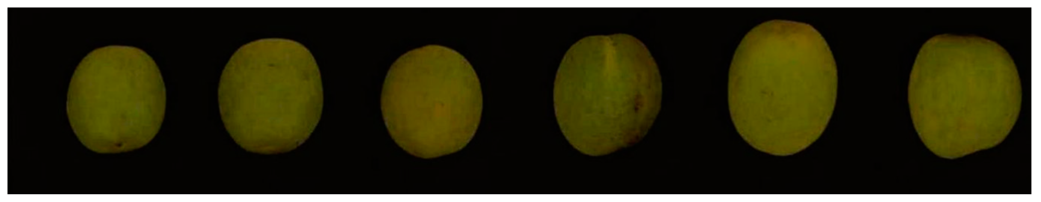
2.1. Green Plum Samples

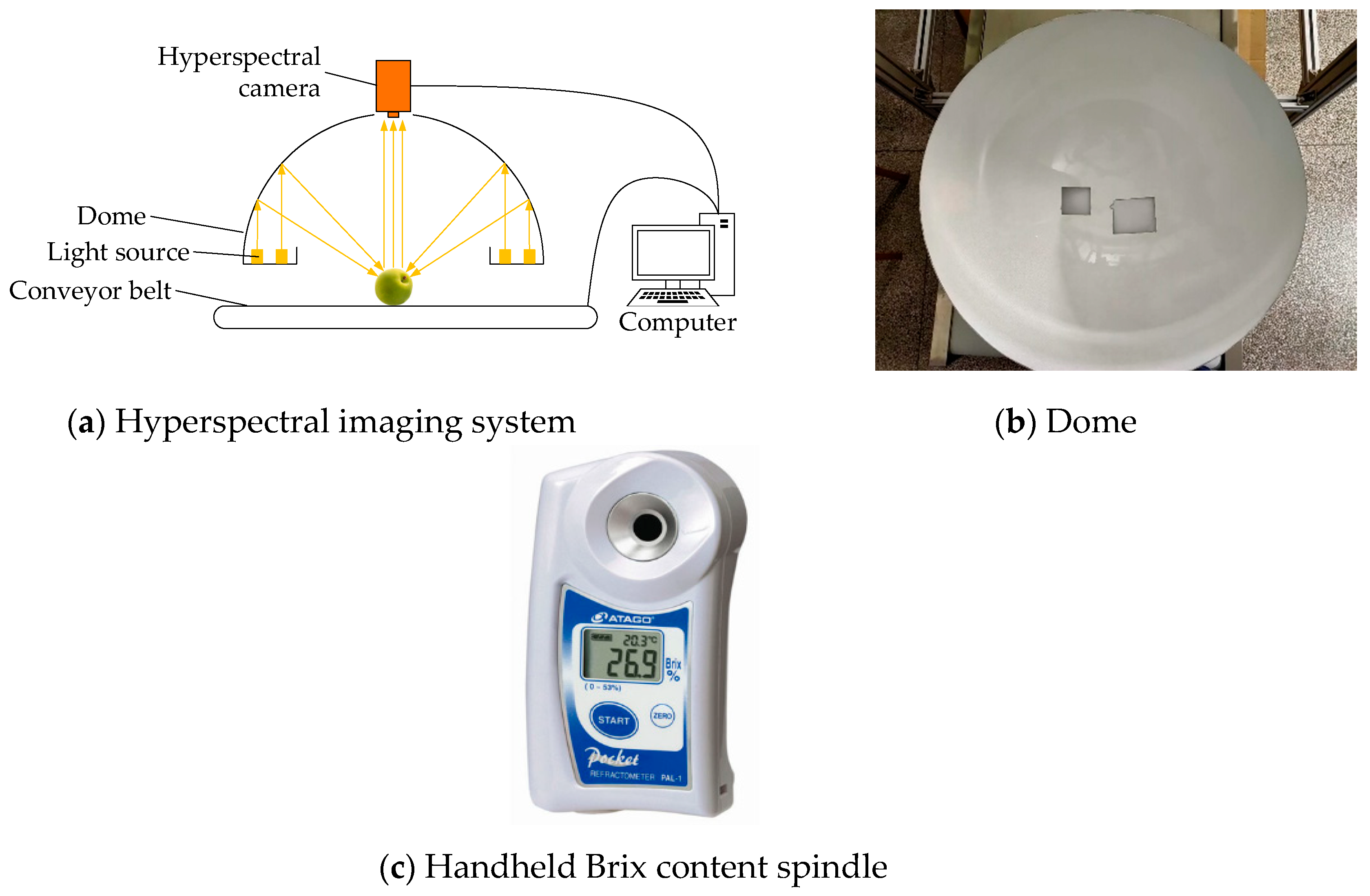
The green plums were purchased from Dali (Yunnan, China). The green plums that are extremely small or have large areas of bad spots and rot were removed. The samples were stored in a laboratory refrigerator maintained at 4 °C. During each test, each sample was randomly selected and placed at room temperature. The spectral data collection and the physicochemical experiments were performed when the fruit temperature was the same as the room temperature.

2.2. Equipment

The GaiaField-V10E-AZ4 visible near-infrared hyperspectral camera of Shuanglihepu Company (Sichuan, China), the main instrument used in the experiments, had a spectral imaging range of 400–1000 nm and a spectral resolution of 2.8 nm.

On the basis of this instrument, a new green plum hyperspectral imaging system was developed. The system consisted of a camera, a light source, a conveyor belt, and a computer, as shown in Figure 1a. The computer controlled the camera and the conveyor belt. The speed of the conveyor belt controlled the camera’s shooting speed, ensuring that the sample smoothly passed through the field of view of the camera and made the obtained data closer to reality. The light emitted by the halogen light source fell on the sample through the reflection of the dome, whose interior is evenly coated with Teflon, ensuring that the light on the sample was as uniform as possible and keeping the light in the camera’s field of view constant, which guaranteed subsequent data processing, as shown in Figure 1b. The SSC was measured using the PAL-1 handheld Brix content spindle, as shown in Figure 1c.

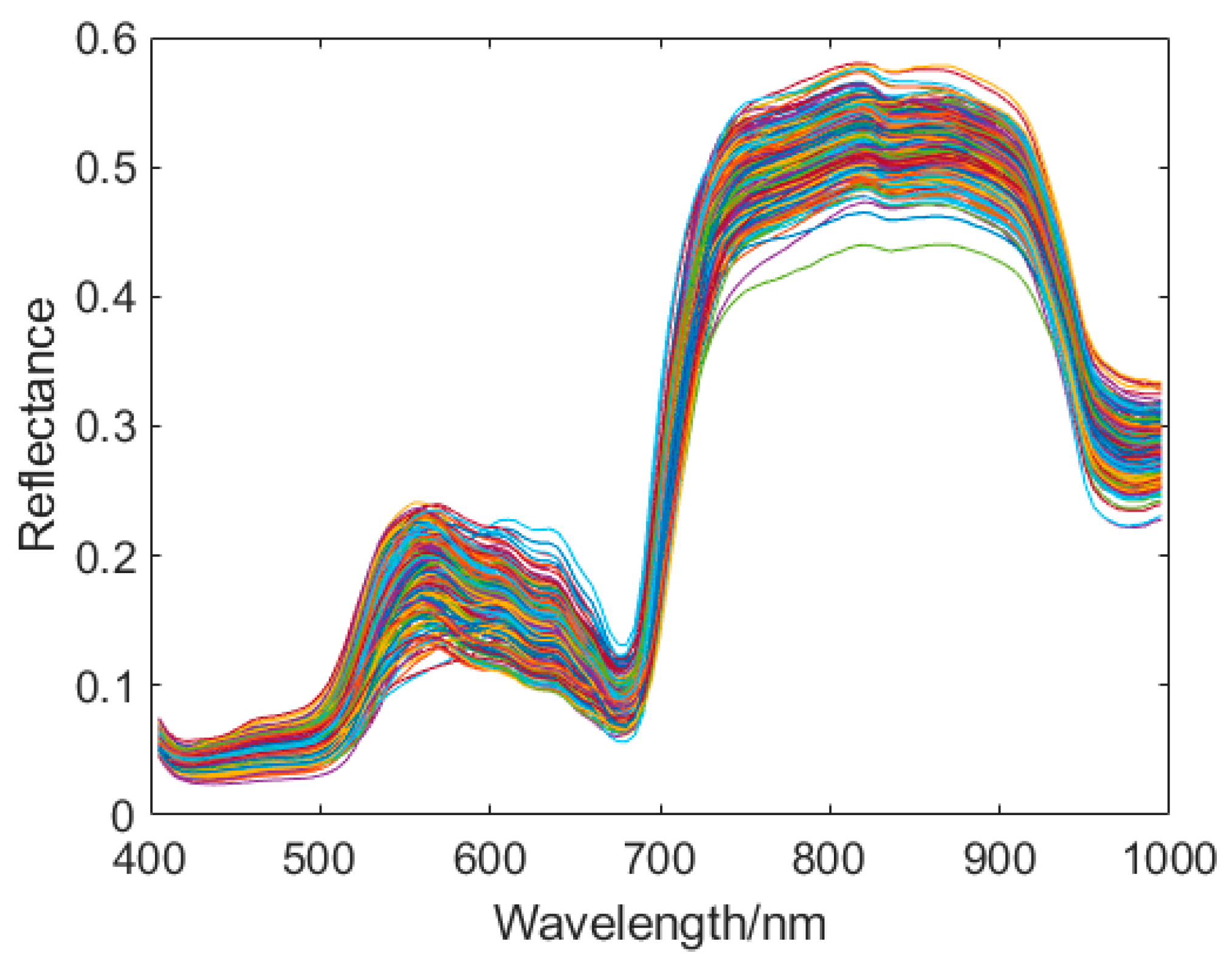
2.3. Hyperspectral Data Acquisition

Before testing, the hyperspectral imaging system was turned on and warmed up for 30 min to determine the best parameters of spectra acquired through the pretest. The exposure time and the moving speed of the conveyor belt were 1.2 ms and 0.6 cm/s, respectively. After scanning the entire green plum, the obtained hyperspectral data were calibrated using standard white and dark reference images. The white reference image is obtained from the 99% standard reflectance plate whose surface is made of Teflon, and this reflectance plate is provided by the camera manufacturer. The dark reference image is obtained after covering the camera lens cap. The calibration image A₀ is defined as:

$$A_0=\frac{A-A_D}{A_W-A_D}\times 100\%$$

(1)

where A₀ is the green plum spectral reflectance data after the calibration, A is the green plum spectral raw data, A_D is the dark field spectral reflectance data, and A_W is the 99% reflectance plate spectral data.

2.4. Green Plum SSC Testing

After the spectral data were collected, the green plum juice was squeezed out of the green plum immediately. The slot of the Brix content spindle was cleaned using distilled water and wiped dry. An appropriate amount of green plum juice was poured into the sample tank to record the SSC value. The SSC of each sample was measured thrice, and their average was set as the SSC value of the sample for subsequent data processing.

There were 366 samples selected and sorted according to the SSC value. One of every four samples was randomly selected as a prediction set sample, and the remaining were used for training. Finally, 274 and 92 samples were selected and constructed as a calibration set and a prediction set, respectively.

Table 1. Soluble solids content (SSC) distributions of green plum.

Sample Set	n	Max	Min	Mean	SD
Calibration set	274	13.1	5.8	9.7	1.768
Prediction set	92	12.4	5.8	9.7	1.819

Note: SD means standard deviation.

shows the measured SSC values of the plum samples.

2.5. Image Processing

The hyperspectral imaging system was used to collect the green plum image. Figure 2 shows the pseudocolor image of the samples. The ENVI5.3 software region of interest tool was used to select the green plum part from the image, and the average spectral reflectance was calculated. The Matlab2016b software was used for pretreatment, modeling, and green plum spectral data analysis. Figure 3 shows the original spectral reflectance curves of all the green plum samples.

3. Model Establishment

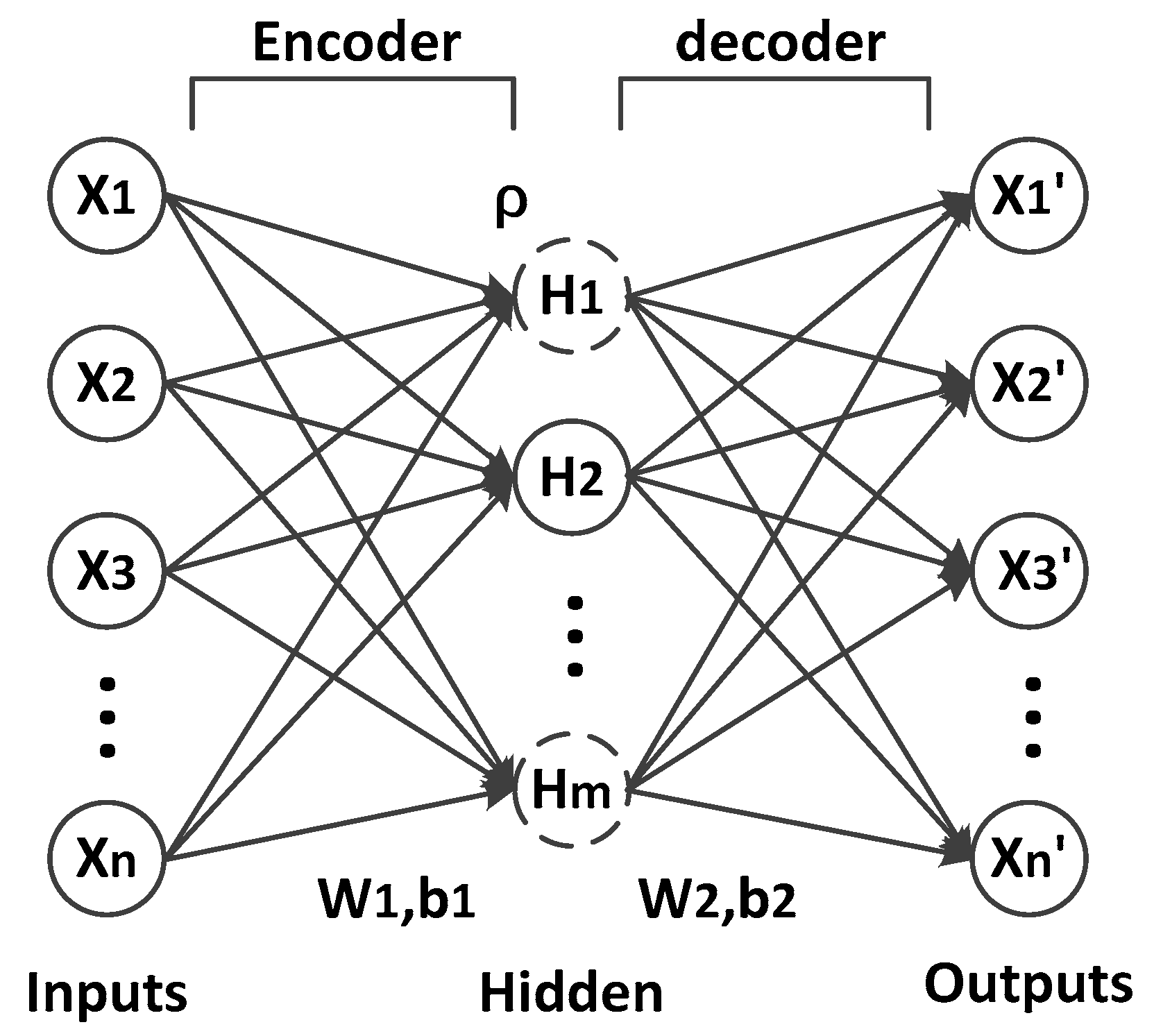
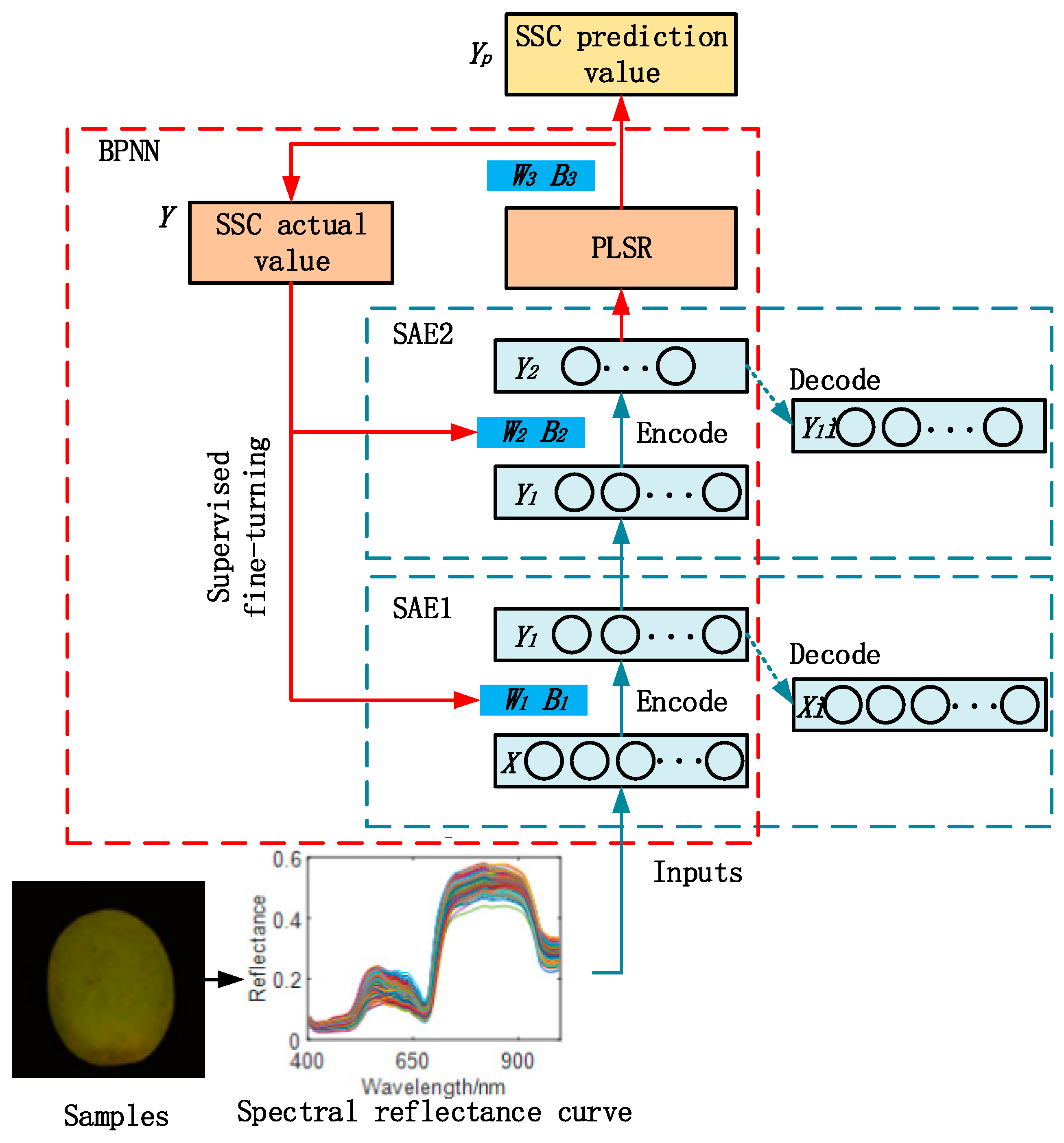
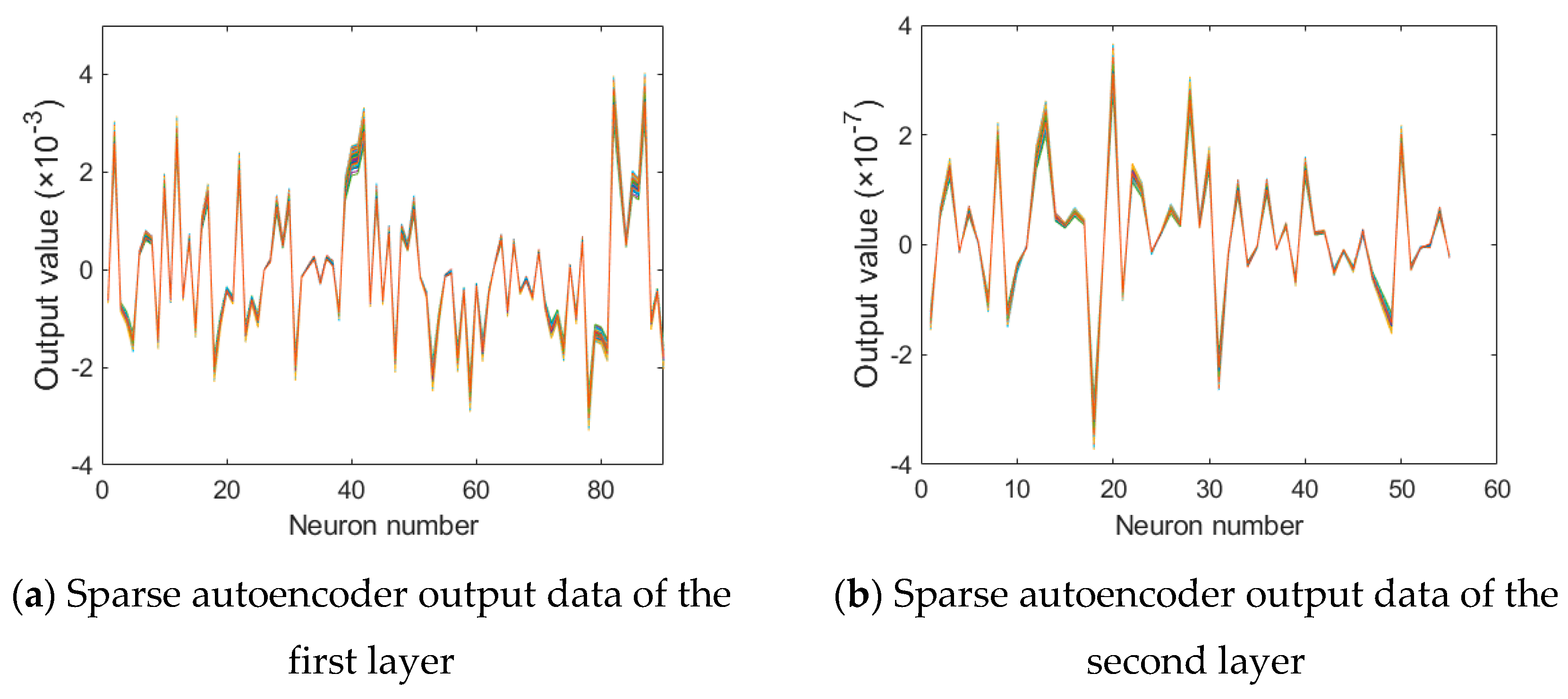
3.1. SAE

The autoencoder, which is usually used for the pretraining of the original high-dimensional data to reduce the data dimension and remove some useless information, is an unsupervised model of artificial intelligence deep learning [23,24]. This model can reduce the subsequent training pressure of the model and improve training accuracy. The autoencoder included an encoder and a decoder.

The autoencoder was used to reconstruct the input data at the output layer and ensure that the output signals [X₁′, X₂′, X₃′, …, X_n′] were exactly the same as the input signals [X₁, X₂, X₃, …, X_n]. The encoding and the decoding processes of the autoencoder are defined as:

$$h=f_e\left(W_{1}x+b_1\right)$$

(2)

$$x^{\prime }=f_d\left(W_{2}h+b_2\right)$$

(3)

where h is the encoded hidden layer feature parameter; W₁ and b₁ are the weight and the offset, respectively, of the encoder; W₂ and b₂ are the weight and the offset, respectively, of the decoder; f_e and f_d are the activation functions of the encoder and the decoder, respectively. The commonly used activation functions are sigmoid, tanh, and Relu.

The definition of the loss function of the autoencoder is given to minimize the difference between the input and output data of the autoencoder.

$$J\left(W,b\right)=\frac{1}{2n}{\displaystyle \sum }_{i=1}^n\Vert x_i{}^{\prime }-x_i\Vert {}^2$$

(4)

where n is the number of input samples, x_i and x_i′ represent the input and the output, respectively, of sample i.

The output of the autoencoder was almost equal to the input. However, the intermediate hidden layer obtained by encoding the input layer can restore the original features after decoding. Therefore, the hidden layer implemented the abstraction of the raw data. The abstraction was another way to represent raw data. When the number of neurons in hidden layer was greater than or equal to the dimension of the input layer, the data were embedded in the neural network mechanically, and features were not extracted. When the number of neurons in the hidden layer was less than the dimension of the input layer, autoencoding can extract the features. Therefore, on the basis of traditional autoencoders, the sparsity restriction was added to the hidden layer neurons to form the SAEs [25,26]. Figure 4 shows the structure of the SAE. Most neurons of the hidden layer in the SAE were restricted, presented as H₁ and H_m in Figure 4.

The sigmoid is an example of an activation function. A neuron was activated when its output was close to 1 and suppressed when its output was close to 0. The sparsity parameter ρ was introduced to suppress the neuron activity. ρ was adopted close to 0 to make the average activation degree of the hidden layer neurons ${\widehat{\rho }}_j$ equal to ρ as much as possible. The sparsity restriction was added to the original autoencoder as an additional penalty factor.

$${\displaystyle \sum }_{j=1}^s\rho \log \frac{\rho }{{\widehat{\rho }}_j}+\left(1-\rho \right)\log \frac{1-\rho }{1-{\widehat{\rho }}_j}$$

(5)

where j stands for each neuron in the hidden layer, s is the number of hidden layer neurons, ${\widehat{\rho }}_j$ is the average activation degree of hidden layer neurons, and ρ is a sparsity parameter.

After adding the sparsity restriction to the SAE, the cost function is defined as:

$$J_{sparse}\left(W,b\right)=\frac{1}{2n}{\displaystyle \sum }_{i=1}^n\Vert x_i{}^{\prime }-x_i\Vert {}^2+\beta \left({\displaystyle \sum }_{j=1}^s\rho \log \frac{\rho }{{\widehat{\rho }}_j}+\left(1-\rho \right)\log \frac{1-\rho }{1-{\widehat{\rho }}_j}\right)$$

(6)

where β is the weight of the sparsity penalty factor.

The sparsity restriction made most of the neurons in the hidden layer restricted. Therefore, the encoding process of the SAE extracted the low-dimensional feature vectors from the high-dimensional data. Through self-learning, the SAE can obtain the effective features from raw data to reduce the data dimension and interference factors of the original information and avoid overfitting caused by excessive high dimensions and problems, such as the collinearity in the raw data.

3.2. SAE–PLSR

Aiming at predicting the SSC in green plum, a multi-layer network model SAE–PLSR was proposed, as shown in Figure 5. The input layer of SAE1 was the input layer of SAE–PLSR, and the hidden layers of SAE1 and SAE2 were the first hidden layer and second hidden layer of SAE–PLSR. PLSR was the third hidden layer of SAE–PLSR. The output of SAE2 hidden layer was passed to the PLSR model and trained. As a statistical regression method, the PLSR model has been widely used in the prediction research by spectral pattern [27,28]. The result of the third hidden layer was directly passed to the output layer as the output result of SAE–PLSR.

SAE uses an unsupervised training method, whose purpose is to reconstruct the input data. In order to improve accuracy, a supervised fine turning was added [29,30]. The results of SAE–PLSR were compared with the actual results, the error was calculated and backpropagated and the parameters in the network were adjusted.

Before network training, the green plum spectral data was pre-trained by SAEs. The weights and offsets of the first hidden layer and second hidden layer 2 of SAE–PLSR were initialized through the weights and offsets obtained by SAEs. During the network training process, the W³ and B³ calculated by the PLSR were updated by the PLSR itself. The updating principle of weights and offsets is based on the back propagation principle, so it can be obtained as follows:

$$\Delta W^i=-\eta \frac{\partial E}{\partial W^i}=-\eta {\delta }^{i+1}{X}^i$$

(7)

$$\Delta B^i=-\eta \frac{\partial E}{\partial B^i}=-\eta {\delta }^{i+1}$$

(8)

where E is the deviation between the output result and the actual result, Wⁱ is the weight transferred from layer i to layer i+1, Bⁱ is the offset transferred from layer i to layer i+1, Xⁱ is the input of layer i, η is the gradient decline proportion coefficient, and δⁱ⁺¹ is calculated by:

$${\delta }^{i+1}={\delta }^{i+2}{W}^{i+1}{f}^{\prime }\left(W^i{X}^i+B^i\right)$$

(9)

The δ⁴ of output layer is calculated by:

$${\delta }^4=-\left(Y_p-Y\right)f^{\prime }\left(W^3{X}^3+B^3\right)$$

(10)

The result of PLSR was directly transferred to the output layer. So the activation function is equivalent to Y = X and its derivatives is calculated by:

$$f^{\prime }\left(W^3{X}^3+B^3\right)=1$$

(11)

The activation function of SAEs is the Sigmod function, so its derivatives is calculated by:

$$f^{\prime }\left(W^i{X}^i+B^i\right)=\left(W^i{X}^i+B^i\right)\left(1-\left(W^i{X}^i+B^i\right)\right)$$

(12)

Since SAE added a penalty term to the cost function, δⁱ⁺¹ was updated as:

$${\delta }^{i+1}={\displaystyle (}\left(\left({\delta }^{i+2}{W}^{i+1}\right)+\beta \left(-\frac{\rho }{\widehat{\rho }}+\frac{1-\rho }{1-\widehat{\rho }}\right)\right){\displaystyle )}{f}^{\prime }\left(W^i{X}^i+B^i\right)$$

(13)

4. Results and Discussion

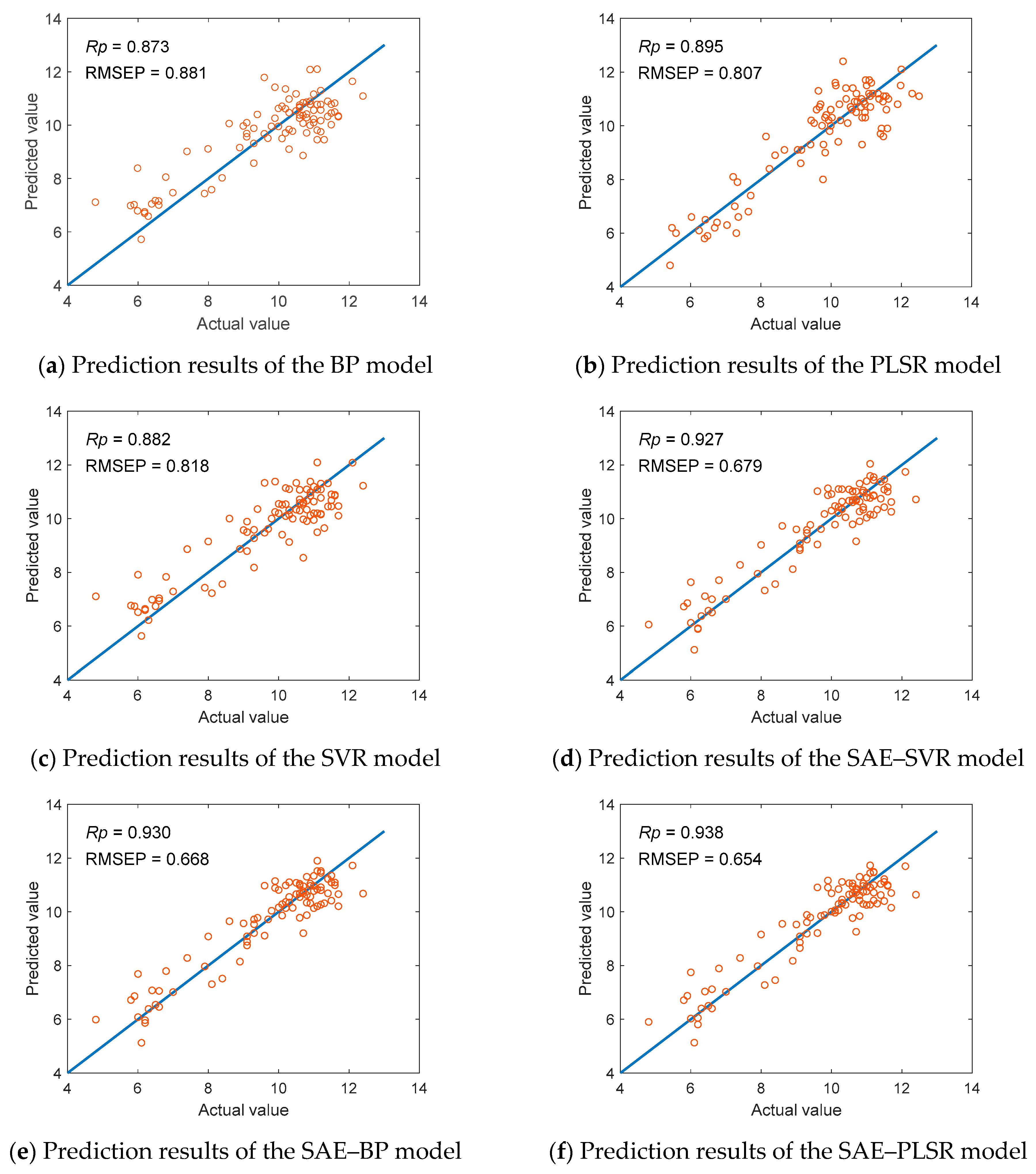
4.1. Performance Analysis of SAE–PLSR Model

The input of SAE–PLSR was a hyperspectral characteristic curve and the corresponding SSC value of a 119-dimensional green plum. The number of neurons in the SAE was set to [90,55] and the sparsity parameter ρ was set to 0.01. The SAE was used to train the raw data beforehand. The hidden layer outputs of the two SAEs are shown in Figure 6.

The correlation coefficient (R) and root mean squared error (RMSE) were used to evaluate the performance of the models. R_C (correlation coefficient in calibration set) and RMSEC (root mean squared error in calibration set) were used to evaluate the performance of the calibration set, whereas R_P (correlation coefficient in prediction set) and RMSEP (root mean squared error in prediction set) were used to evaluate the performance of the prediction set. After training, the prediction performance of the SAE–PLSR model on green plum was quantified, the R_C, RMSEC, R_P, and RMSEP values were 0.957, 0.542, 0.938, and 0.654, respectively.

In order to evaluate the performance of the present model, the SAE–PLSR model was compared with three traditional methods, namely, BP neural network [31], SVR machine [32], and PLSR [33] to reflect prediction performance. For these methods, Li et al. [34] have used PLSR model to predict the SSC of plum with the short wave near infrared hyperspectral image and obtained good prediction results. Figure 7 shows the prediction results of different models and

Table 2. Comparison of the prediction performance of the SAE–PLSR and the traditional models.

Model	RC	RMSEC	RP	RMSEP
BP	0.886	0.820	0.873	0.881
SVR	0.894	0.628	0.882	0.818
PLSR	0.968	0.442	0.895	0.807
SAE–BP	0.942	0.582	0.930	0.668
SAE–SVR	0.939	0.602	0.927	0.679
SAE–PLSR	0.957	0.542	0.938	0.654

shows the results of the comparison between the SAE–PLSR model and other traditional models.

The results of the comparison showed that the PLSR model had good prediction performance on the calibration set. However, the prediction performance on the prediction set was not good enough. Compared with the calibration set, the prediction set had a 82.6% increase in RMSEP and 7.5% decrease in R_P, indicating that the robustness of the PLSR model was not good or that overfitting occurred. The SVR and the BP models were inferior to the PLSR model in prediction performance. The R_P for the prediction sets of the SVR and the BP models decreased by 1.5% and 2.5%, respectively, and the RMSEP for the prediction sets of the SVR and the BP models increased by 1.4% and 9.2%, respectively. The prediction performance of the SAE–PLSR model greatly improved compared with that of the PLSR model. The calibration set had a 1.1% decrease in R_C and a 22.6% increase in RMSEC. The main reason for the analysis results was that the input of the PLSR model was the raw spectral pattern of green plum, which contained 119-dimensional data. The SAE–PLSR model only had a PLSR module input of only 55-dimensional data. Therefore, the calibration set of the SAE–PLSR model was not as effective as that of the PLSR model. However, the prediction set of SAE–PLSR model had better performance compared with that of the PLSR model, the R_P increased by 4.8% and the RMSEP decreased by 19.0%. Meanwhile, the PLSR model in the SAE–PLSR model was replaced with BP and SVR for prediction and analysis. The experiment found that the prediction effect of the two models was not as good as SAE–PLSR. The R_P of the SAE–BP and the SAE–SVR models decreased by 0.9% and 1.2%, respectively, and the RMSEP of the SAE–BP and the SAE–SVR models increased by 2.1% and 3.8%. These results indicated that the SAE–PLSR model had good performance in the green plum SSC prediction.

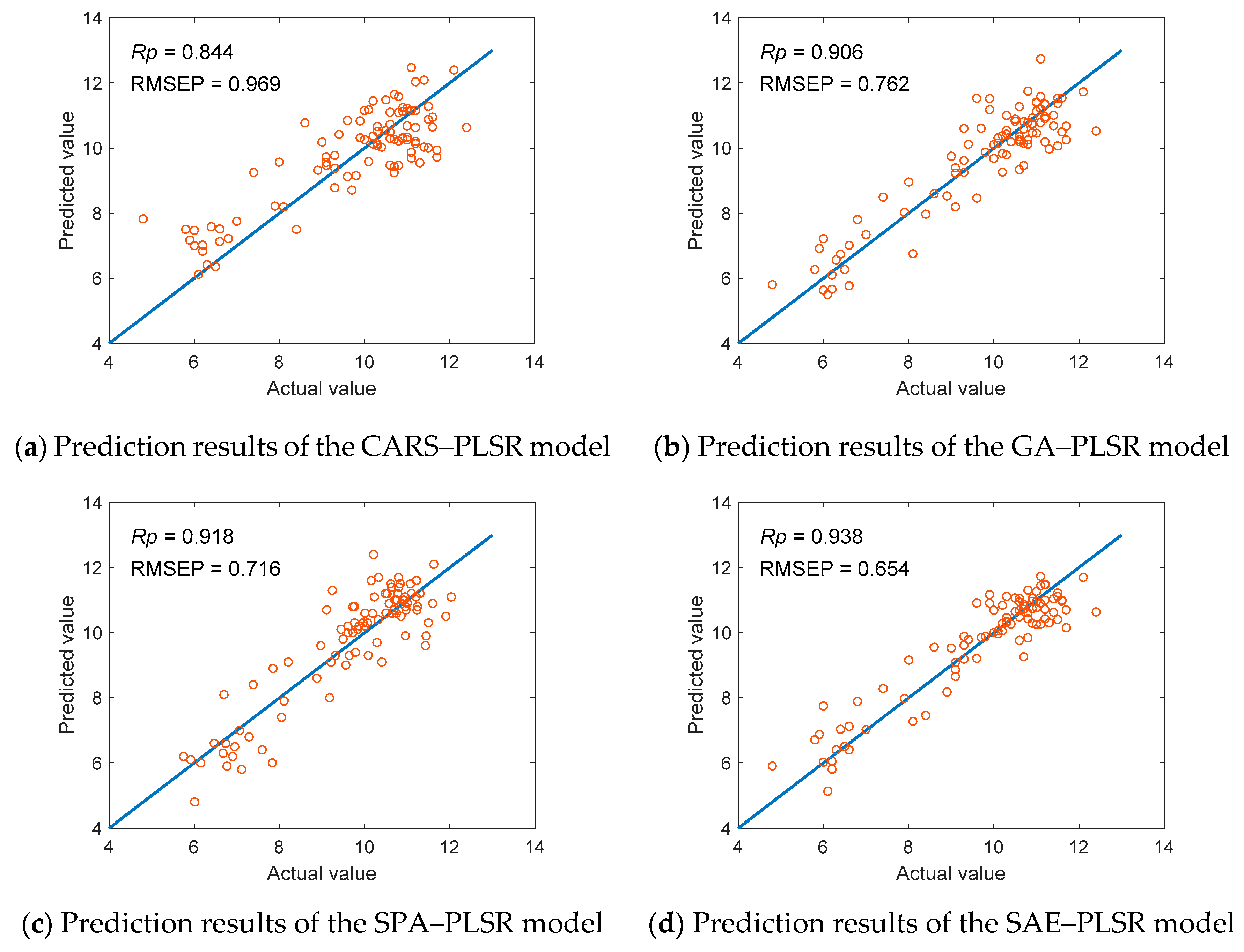
4.2. Performance Analysis of Feature Extraction Methods

The SNR of some bands in the hyperspectral data was relatively low because of the influence of noise. At the same time, a linear correlation or redundant information between the data in different bands may exist. Modeling with the whole band may lower the prediction accuracy of the model. Therefore, the method of extracting feature wavelengths can eliminate some of the band information and improve the prediction performance of the model [35]. The training process of the SAE was the process of extracting features from the raw data. The output of the hidden layer also completed the function of dimension reduction on the basis of feature extraction. PLSR was used as the prediction model in this study. Three feature wavelength extraction methods, namely, SPA, CARS, and genetic algorithm, were selected and integrated with PLSR. The three integrated models were compared with the SAE–PLSR model. Figure 8 shows the prediction results of the different models.

Table 3. Comparison of the prediction performance of the SAE–PLSR and the traditional integrated models.

Model	RC	RMSEC	RP	RMSEP
SPA–PLSR	0.925	0.675	0.918	0.716
CARS–PLSR	0.869	0.870	0.844	0.969
GA–PLSR	0.955	0.526	0.906	0.762
SAE–PLSR	0.957	0.542	0.938	0.654

shows the results of comparison of the different models.

Table 3 shows that the CARS method had poor performance on the green plum SSC prediction. The prediction accuracy of the CARS method was lower than that of the simple PLSR model. Compared with that of the PLSR model, the prediction set of the CARS method had a 5.7% decrease in R_P and a 20.1% increase in RMSEP. The SPA and the GA methods had good performance on reducing the data dimension and improving prediction performance. The R_P for the prediction set of the SPA and the GA methods increased by 2.6% and 1.2%, respectively, and the RMSEP for the prediction set of the SPA and the GA methods decreased by 11.3% and 5.6%, respectively. Compared with the previous two methods, the SAE–PLSR model still had better prediction performance. For feature wavelength extraction, the prediction set of the SAE–PLSR model had a 2.2% increase in R_P and an 8.7% decrease in RMSEP compared with that of the SPA–PLSR. The green plum SSC prediction verified the SAE–PLSR model.

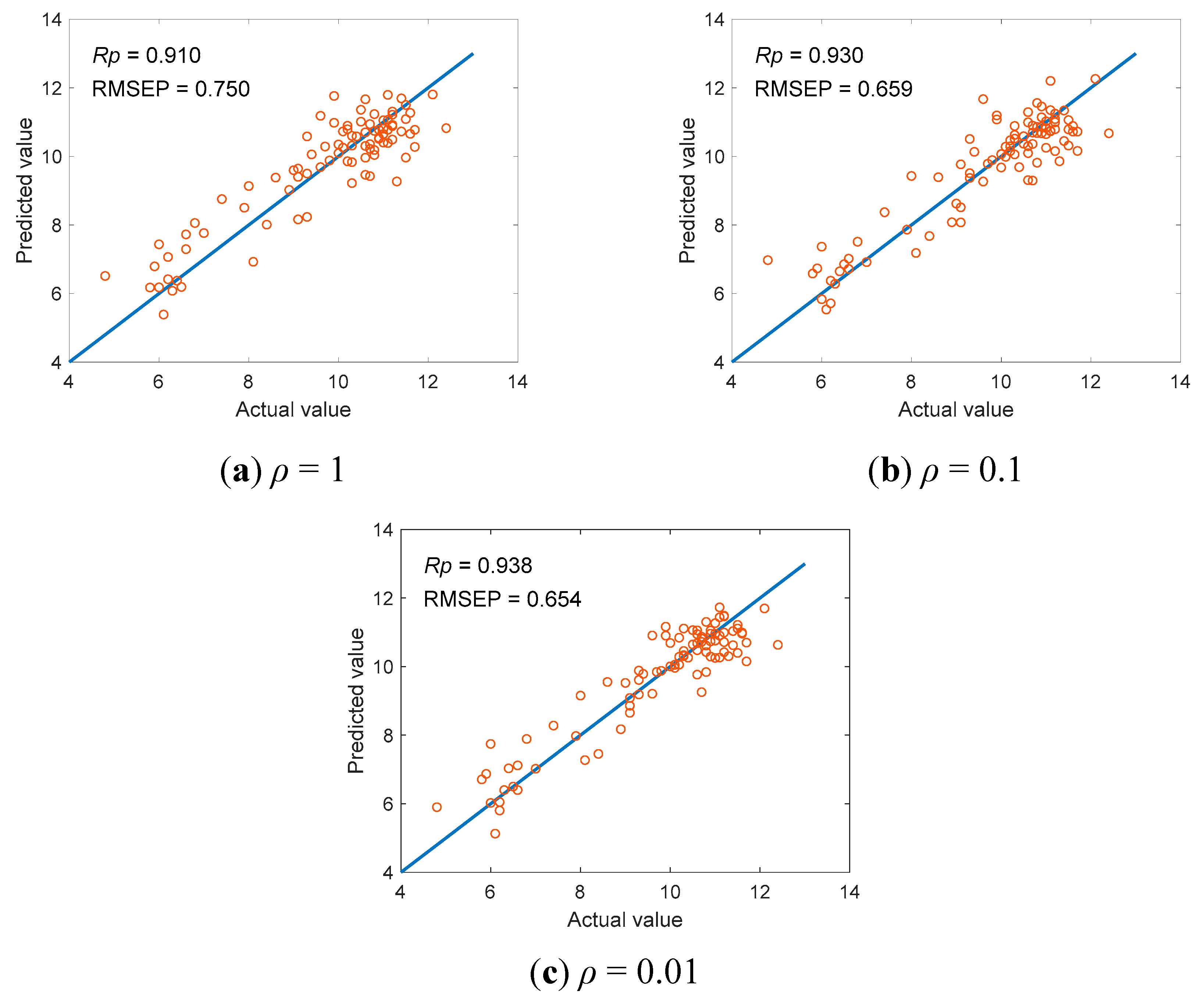
4.3. Influence of Sparsity Parameter ρ on Prediction Results

The sparsity parameter ρ plays a key role in model training. Different sparsity parameters determine the degree of neuron activation. In order to explore the influence of sparsity parameters on the prediction results of the model, three different sparsity parameters of 0.01, 0.1, and 1 were selected for modeling. Figure 9 shows the prediction results of the different models. The results is shown in

Table 4. Comparison of the prediction performance of three different sparsity parameters (ρ).

ρ	RC	RMSEC	RP	RMSEP
1	0.929	0.633	0.910	0.750
0.1	0.949	0.574	0.930	0.659
0.01	0.957	0.542	0.938	0.654

. When the sparsity parameter is 1, the neurons are activated without any restriction, which has R_P and RMSEP values of 0.910 and 0.750, respectively. When the sparsity parameter is 0.1, compared with that of 1, the model prediction performance is improved, which has a 2.2% increase in R_P and a 12.1% decrease in RMSEP. When the sparsity parameter is 0.01, compared with that of 1, the model prediction performance is further improved, which has a 3.1% increase in R_P and a 12.8% decrease in RMSEP. This shows that the sparsity parameter can affect the SAE–PLSR model prediction performance. The reason may be that the sparsity restriction is added, so that most of the useless features and the features that are harmful to the model prediction are inhibited, and the influence of the useful features is amplified [36]. So, the prediction accuracy of the model is improved. In this paper, the sparsity parameter 0.01 is used to effectively improve the model prediction performance.

5. Conclusions

SSC is one of the important indicators in the processing of green plums. The hyperspectral technology is used for testing to achieve the nondestructive testing of SSC. On the basis of the newly developed hyperspectral imaging system, the spectroscopic data of green plum are collected. Experimental analysis has proven that the use of visible–infrared spectroscopy can effectively predict the SSC in plums. The spectral information of 400–1000 nm is collected, and the SSC prediction is performed using the PLSR model, which has R_P and RMSEP values of 0.895 and 0.807, respectively. The SAE–PLSR model is proposed on the basis of the traditional unsupervised learning models to improve the prediction accuracy of green plum SSC. The autoencoder is improved, and the multilayer SAEs are connected. Moreover, the PLSR module is used for regression prediction to back propagate the predicted error, adjust the model parameters, and improve the model prediction performance. The results of the experiment prove that compared with the traditional PLSR model, the SAE–PLSR model prediction set has a 4.8% increase in R_P and a 19.0% decrease in RMSEP. The model also has advantages compared with the traditional feature extraction and regression prediction methods. By comparison, the prediction set has a 2.2% increase in R_P and an 8.7% decrease in RMSEP. The SAE–PLSR model has good prediction performance on green plum SSC. However, the training time of the model has increased because of the multiple back-propagation processes. The model can still be improved later to reduce the training time of the model.

References

1. Wang, X.; Matetić, M.; Zhou, H.; Zhang, X.; Jemrić, T. Postharvest Quality Monitoring and Variance Analysis of Peach and Nectarine Cold Chain with Multi-Sensors Technology. Appl. Sci. 2017, 7, 133. [Google Scholar] [CrossRef] [Green Version]
2. Xiao, H.; Feng, L.; Song, D.; Tu, K.; Peng, J.; Pan, L. Grading and Sorting of Grape Berries Using Visible-Near Infrared Spectroscopy on the Basis of Multiple Inner Quality Parameters. Sensors 2019, 19, 2600. [Google Scholar] [CrossRef] [PubMed] [Green Version]
3. Huang, Y.; Liu, Y.; Yang, Y.; Zhang, Z.; Chen, K. Assessment of Tomato Color by Spatially Resolved and Conventional Vis/NIR Spectroscopies. Spectrosc. Spectr. Anal. 2019, 39, 3585–3591. [Google Scholar]
4. Huang, Y.; Lu, R.; Chen, K. Assessment of Tomato Soluble Solids Content and pH by Spatially-Resolved and Conventional Vis/NIR Spectroscopy. J. Food Eng. 2018, 236, 19–28. [Google Scholar] [CrossRef]
5. Huang, Y.; Lu, R.; Chen, K. Detection of Internal Defect of Apples by a Multichannel Vis/NIR spectroscopic system. Postharvest Biol. Technol. 2020, 116, 111065. [Google Scholar] [CrossRef]
6. Ni, C.; Wang, D.; Tao, Y. Variable Weighted Convolutional Neural Network for the Nitrogen Content Quantization of Masson Pine Seedling Leaves with Near-Infrared Spectroscopy. Spectrochim. Acta Part A Mol. Biomol. Spectrosc. 2019, 209, 32–39. [Google Scholar] [CrossRef]
7. Cheng, W.; Sun, D.W.; Pu, H. Heterospectral Two-Dimensional Correlation Analysis with Near-Infrared Hyperspectral Imaging for Monitoring Oxidative Damage of Pork Myofibrils During Frozen Storage. Food Chem. 2018, 248, 119–127. [Google Scholar] [CrossRef]
8. Wang, X.; An, S.; Xu, Y.; Hou, H.; Chen, F.; Yang, Y.; Zhang, S.; Liu, R. A Back Propagation Neural Network Model Optimized by Mind Evolutionary Algorithm for Estimating Cd, Cr, and Pb Concentrations in Soils Using Vis-NIR Diffuse Reflectance Spectroscopy. Appl. Sci. 2020, 10, 51. [Google Scholar] [CrossRef] [Green Version]
9. Zheng, X.; Peng, Y.; Wang, W. A Nondestructive Real-Time Detection Method of Total Viable Count in Pork by Hyperspectral Imaging Technique. Appl. Sci. 2017, 7, 213. [Google Scholar] [CrossRef] [Green Version]
10. Caporaso, N.; Whitworth, M.B.; Fisk, I.D. Protein Content Prediction in Single Wheat Kernels Using Hyperspectral Imaging. Food Chem. 2018, 240, 32–42. [Google Scholar] [CrossRef]
11. Lu, X.; Sun, J.; Mao, H.; Wu, X.; Gao, H. Quantitative Determination of Rice Starch Based on Hyperspectral Imaging Technology. Int. J. Food Prop. 2017, 20 (Suppl. S1), S1037–S1044. [Google Scholar] [CrossRef]
12. Zhou, F.; Peng, J.; Zhao, Y.; Huang, W.; Jiang, Y.; Li, M.; Wu, X.; Lu, B. Varietal Classification and Antioxidant Activity Prediction of Osmanthus Fragrans Lour. Flowers Using UPLC–PDA/QTOF–MS and Multivariable Analysis. Food Chem. 2017, 217, 490–497. [Google Scholar] [CrossRef] [PubMed]
13. Krepper, G.; Romeo, F.; Fernandes, D.; Diniz, P.; de Araujo, M.; Di Nezio, M.; Pistonesi, M.; Centurion, M. Determination of Fat Content in Chicken Hamburgers Using NIR Spectroscopy and the Successive Projections Algorithm for Interval Selection in PLS Regression (iSPA-PLS). Spectrochim. Acta Part A Mol. Biomol. Spectrosc. 2018, 189, 300–306. [Google Scholar] [CrossRef] [PubMed]
14. Zhu, T.; Xie, L.; Wei, H.; Wang, H.; Zhao, X.; Zhang, K. Clear-sky Direct Normal Irradiance Estimation Based on Adjustable Inputs and Error Correction. J. Renew. Sustain. Energy 2019, 11, 056101. [Google Scholar] [CrossRef]
15. Weng, S.; Guo, B.; Tang, P.; Yin, X.; Pan, F.; Zhao, J.; Huang, L.; Zhang, D. Rapid Detection of Adulteration of Minced Beef Using Vis/NIR Reflectance Spectroscopy with Multivariate Methods. Spectrochim. Acta Part A Mol. Biomol. Spectrosc. 2020, 230, 118005. [Google Scholar] [CrossRef]
16. Deng, F.; Pu, S.; Chen, X.; Shi, Y.; Yuan, T.; Pu, S. Hyperspectral Image Classification with Capsule Network Using Limited Training Samples. Sensors 2018, 18, 3153. [Google Scholar] [CrossRef] [Green Version]
17. Liu, L.; Ji, M.; Buchroithner, M. Transfer Learning for Soil Spectroscopy Based on Convolutional Neural Networks and Its Application in Soil Clay Content Mapping Using Hyperspectral Imagery. Sensors 2018, 18, 3169. [Google Scholar] [CrossRef] [Green Version]
18. Li, K.; Wang, M.; Liu, Y.; Yu, N.; Lan, W. A Novel Method of Hyperspectral Data Classification Based on Transfer Learning and Deep Belief Network. Appl. Sci. 2019, 9, 1379. [Google Scholar] [CrossRef] [Green Version]
19. Sun, W.; Shao, S.; Zhao, R.; Yan, R.; Zhang, X.; Chen, X. A Sparse Auto-encoder-Based Deep Neural Network Approach for Induction Motor Faults Classification. Measurement 2016, 89, 171–178. [Google Scholar] [CrossRef]
20. Li, S.; Yu, B.; Wu, W.; Su, S.; Ji, R. Feature Learning Based on SAE–PCA Network for Human Gesture Recognition in RGBD Images. Neurocomputing 2015, 151, 565–573. [Google Scholar] [CrossRef]
21. Han, X.; Zhong, Y.; Zhang, L. Spatial-spectral Unsupervised Convolutional Sparse Auto-encoder Classifier for Hyperspectral Imagery. Photogramm. Eng. Remote Sens. 2017, 83, 195–206. [Google Scholar] [CrossRef]
22. Fan, Y.; Zhang, C.; Liu, Z.; Qiu, Z.; He, Y. Cost-sensitive Stacked Sparse Auto-encoder Models to Detect Striped Stem Borer Infestation on Rice Based on Hyperspectral Imaging. Knowl.-Based Syst. 2019, 168, 49–58. [Google Scholar] [CrossRef]
23. Peng, X.; Feng, J.; Xiao, S.; Yan, W.; Zhou, J.; Yang, S. Structured AutoEncoders for Subspace Clustering. IEEE Trans. Image Process. 2018, 27, 5076–5086. [Google Scholar] [CrossRef] [PubMed]
24. Blaschke, T.; Olivecrona, M.; Engkvist, O.; Bajorath, J.; Chen, H. Application of Generative Autoencoder in de Novo Molecular Design. Mol. Inform. 2017, 37, 1700123. [Google Scholar] [CrossRef] [PubMed] [Green Version]
25. Wen, L.; Gao, L.; Li, X. A New Deep Transfer Learning Based on Sparse Auto-Encoder for Fault Diagnosis. IEEE Trans. Syst. Man Cybern. Syst. 2017, 49, 136–144. [Google Scholar] [CrossRef]
26. Luo, X.; Xu, Y.; Wang, W.; Yuan, M.; Ban, X.; Zhu, Y.; Zhao, W. Towards Enhancing Stacked Extreme Learning Machine with Sparse Autoencoder by Correntropy. J. Frankl. Inst. 2017, 355, 1945–1966. [Google Scholar] [CrossRef]
27. Wang, X.; Zhao, M.; Ju, R.; Song, Q.; Hua, D.; Wang, C.; Chen, T. Visualizing quantitatively the freshness of intact fresh pork using acousto-optical tunable filter-based visible/near-infrared spectral imagery. Comput. Electron. Agric. 2013, 99, 41–53. [Google Scholar] [CrossRef]
28. Xu, S.; Zhao, Y.; Wang, M.; Shi, X. Comparison of Multivariate Methods for Estimating Selected Soil Properties from Intact Soil Cores of Paddy Fields by Vis–NIR Spectroscopy. Geoderma 2018, 310, 29–43. [Google Scholar] [CrossRef]
29. Ni, C.; Zhang, Y.; Wang, D. Moisture Content Quantization of Masson Pine Seedling Leaf Based on Stacked Autoencoder with Near-Infrared Spectroscopy. J. Electr. Comput. Eng. 2018, 1–8. [Google Scholar] [CrossRef]
30. Ni, C.; Li, Z.; Zhang, X.; Sun, X.; Huang, Y.; Zhao, L.; Zhu, T.; Wang, D. Online Sorting of the Film on Cotton Based on Deep Learning and Hyperspectral Imaging. IEEE Access 2020. [Google Scholar] [CrossRef]
31. Wang, X.; Wang, X.; Zhang, F.; Ding, J.; Kung, H.; Latif, A.; Johnson, V. Estimation of Soil Salt Content (SSC) in The Ebinur Lake Wetland National Nature Reserve (ELWNNR), Northwest China, Based on a Bootstrap-BP Neural Network Model and Optimal Spectral Indices. Sci. Total Environ. 2018, 615, 918–930. [Google Scholar] [CrossRef] [PubMed]
32. Zhang, N.; Liu, X.; Jin, X.; Li, C.; Wu, X.; Yang, S.; Ning, J.; Yanne, P. Determination of Total Iron-reactive Phenolics, Anthocyanins and Tannins in Wine Grapes of Skins and Seeds Based on Near-infrared Hyperspectral Imaging. Food Chem. 2017, 237, 811–817. [Google Scholar] [CrossRef] [PubMed]
33. Xu, J.; Riccioli, C.; Sun, D. Comparison of Hyperspectral Imaging and Computer Vision for Automatic Differentiation of Organically and Conventionally Farmed Salmon. J. Food Eng. 2017, 196, 170–182. [Google Scholar] [CrossRef]
34. Li, B.; Cobo-Medina, M.; Lecourt, J.; Harrison, N.; Harrison, R.; Cross, J. Application of Hyperspectral Imaging for Nondestructive Measurement of Plum Quality Attributes. Postharvest Biol. Technol. 2018, 141, 8–15. [Google Scholar] [CrossRef]
35. Tang, G.; Huang, Y.; Tian, K.; Song, X.; Yan, H.; Hu, J.; Xiong, Y.; Min, S. A New Spectral Variable Selection Pattern Using Competitive Adaptive Reweighted Sampling Combined with Successive Projections Algorithm. Analyst 2014, 139, 4894. [Google Scholar] [CrossRef]
36. Tang, J.; Deng, C.; Huang, G. Extreme Learning Machine for Multilayer Perceptron. IEEE Trans. Neural Netw. Learn. Syst. 2015, 27, 809–821. [Google Scholar] [CrossRef]
Figure 1. Hyperspectral imaging system, dome, and handheld Brix content spindle.
Applsci 10 03769 g001
Figure 2. Pseudocolor images of some samples.
Applsci 10 03769 g002
Figure 3. Original spectral reflectance curve of plum samples.
Applsci 10 03769 g003
Figure 4. Structure of the sparse autoencoder.
Applsci 10 03769 g004
Figure 5. Structure of the sparse autoencoder–partial least squares regression (SAE–PLSR).
Applsci 10 03769 g005
Figure 6. Sparse autoencoder output data.
Applsci 10 03769 g006
Figure 7. Comparison of the prediction results of the SAE–PLSR and the traditional models.
Applsci 10 03769 g007
Figure 8. Comparison of the prediction results of the SAE–PLSR and the traditional integrated models.
Applsci 10 03769 g008
Figure 9. The prediction results of the SAE–PLSR with different sparsity parameters (ρ).
Applsci 10 03769 g009